Parametrization of the NRTL Model with a Multiobjective Approach: Implications in the Process Simulation

Abstract

Thermodynamics, as a scientific tool, advises on the control of variables involved in processes of different nature and is particularly useful in the design of equipment, or to obtain previous simulations. However, to generate more accurate models, an exact science is required. Thus, the thermodynamic–mathematical binomial is able to relate the fundamental variables of a system using the potential functions directing the process, although these relationships are not always completely satisfactory, as it is necessary to complete the modelling with a set of parameters, which depend on the experimentation. To ensure a better description of the behavior of a system, in this work a multi-objective optimization procedure (MOP) is applied to the NRTL model, comparing the results with other conventional procedures used to characterize the real properties of the binary methyl methanoate + pentane. The results obtained with the MOP confirmed a better representation of the experimental information with NRTL, analyzing its impact on the simulation/design processes. The set of optimal parametrizations obtained allow several options to be process engineered to select the most appropriate one depending on the specific problem to be designed.

1. Introduction

The simulation and design of unitary operations raised for the chemical industry require a prior description of the behavior using its characterization through properties of a different nature: physical, chemical, or those linked to transport phenomena, among others. It is essential to check the viability of a certain process in order to know its directionality and the maximum extension it can reach, as well as the energy exchanges taking place. This is done with thermodynamic analysis [1] of the process under study. When considering the balances involved in the separation operations, it is assumed that the process entails a sequence of equilibrium stages between phases [2] (see Figure 1).

Therefore, a mathematical formalism is required to describe the behavior of the variables involved in the equilibria between phases. The modelling achieved and its implementation in the current process simulation tools allow for the evaluation of “design parameters” such as recovery percentages, products purity, energy requirements, and the size of the equipment, among others. A mathematical–thermodynamics binomial is constituted as a tool that facilitates the modelling of the behavior of the material in the proposed process. Thermodynamic properties are generated by accumulating several effects, some mainly due to temperature and pressure conditions, and others to the molecular interactions in the material. In short, it is necessary to generate a model that quantifies a relationship between the state variables Ξ and those corresponding to the material, F(Ξ) = 0, i.e.,: the equation of state.

Numerous proposals are made in the literature to achieve an appropriate function, which, starting from molecular concepts, is resolved using different theoretical approaches. However, only some of them present a sufficient level of development to become useful tools in the practical engineering calculations. A simple classification groups them as (a) random mixing models [3,4], (b) local composition models [5,6], (c) cubic equations of state [7,8,9], (d) quantum chemistry-based models [10,11,12], and (e) models based on perturbation theory [13,14,15]. However, the different theories fail to accurately represent the real behavior of the material in a wide range of conditions, compensating for the defects observed in the model by introducing a number of adjustable parameters (represented by the vector θ), which constitute the degrees of freedom. Therefore, the homogeneous function that relates the state variables of the system is now F(Ξ,θ) = 0, particularly for the case of multicomponent solutions F(p,T,x,θ) = 0. The parameters θ are defined in relation to the available experimental information, so if the number of parameters in a model increases (↑) and its generality decreases (↓), the greater (↑) its predictive capacity.

In the last 30 years, the models most used in thermodynamic calculations and in chemical engineering applications have been those classified in (b), such as NRTL [5] and UNIQUAC [6]. The latter was derived later in the UNIFAC method [16], with a correlative/predictive character, although the same did not occur with the NRTL model (see Appendix A). If the model is used for both correlative and predictive applications, the parametrization requires previous experimental data of the solutions under study. It is also important to note that the ability of a model to represent the behavior of a material depends not only on its theoretical level, but also on the procedure used to define its parameters or degrees of freedom θ.

This work presents a comprehensive view of the modelling processes of phase equilibria and other properties, reviewing and comparing some commonly used parametrization processes. The approach proposed here is based on the multi-objective optimization methodology, noted as MOP [17], to extensively characterize the properties of solutions [18,19,20,21,22,23]. To illustrate this approach, Figure 2 shows a scheme of the different options used and compared to a real dataset obtained for the methyl methanoate + pentane system, including liquid–liquid equilibrium (LLE) data [24], vapor–liquid equilibrium (VLE), and the mixing energetic effects (h^E) [25]. The diverse information available is one of the reasons for the choice. In the proposed development, different strategies are used to adequately define the parametrization of the NRTL model when applying it to the mentioned system, providing information on the validity range of the parametrizations in relation to the procedure used to obtain them.

2. Parametrization of Thermodynamic Models

Parametrization consists of defining the numerical values of a set of parameters θ, (in the case of the NRTL model: θ = {$\Delta g_{\mathrm{ij}}^{(\mathrm{k})}$, $\Delta g_{\mathrm{ji}}^{(\mathrm{k})}$, ${\alpha }_{12}$} (see Appendix A)) so that the model describes the behavior of the modeled system with the most accuracy. Several parametrization procedures are shown here, including the multi-objective optimization approach, which is particularly suitable when the theoretical level of the model limits the behavior description.

2.1. Conventional Procedure

In practice, if experimental observations are available, a model can be achieved to represent the behavior of the solutions, although practically. Hence, the parametrization is proposed as an optimization problem to minimize the differences between the experimental values and those calculated by the model. This is evaluated by an appropriate metric whose generic approach is:

$$\begin{array}{l}\underset{\mathsf{\theta }}{\min }\delta (\mathsf{\theta }|Y^{\exp },x^{\exp })\\ \mathrm{s}.\mathrm{t}. A\mathsf{\theta }\le b\\ \hspace{0.17em}\hspace{0.17em}\hspace{0.17em}\hspace{0.17em}\hspace{0.17em}\hspace{0.17em}\hspace{0.17em}\hspace{0.17em}\hspace{0.17em}g(\mathsf{\theta }|Y^{\exp },x^{\exp })\le 0\\ \hspace{0.17em}\hspace{0.17em}\hspace{0.17em}\hspace{0.17em}\hspace{0.17em}\hspace{0.17em}\hspace{0.17em}\hspace{0.17em}\hspace{0.17em}h(\mathsf{\theta }|Y^{\exp },x^{\exp })=0\\ \hspace{0.17em}\hspace{0.17em}\hspace{0.17em}\hspace{0.17em}\hspace{0.17em}\hspace{0.17em}\hspace{0.17em}\hspace{0.17em}\hspace{0.17em}\mathsf{\theta }\in P\hspace{0.17em}\hspace{0.17em}\hspace{0.17em}\hspace{0.17em}\hspace{0.17em}\end{array}$$

(1)

where A and b are, respectively, the coefficient matrix and independent terms of the linear constraints to which the problem is subjected; g(θ|Y^exp,x^exp) and h(θ|Y^exp,x^exp) denote the non-linear constraints; and P defines the domain of the model parameters. The space generated to check the constraints of the problem is the feasible space Ω. If the model parameters have a physical significance, the domain can be established considering that significance. For example, in the NRTL model, the non-randomness parameter was established in its first applications with values of α₁₂ ∈ (0.2–0.4) [26], although the minimum interval could also be close to zero, as verified in this work, and even in many cases α₁₂ > 1.

The way in which the metric δ(θ|Y^exp x^exp) is defined affects the applicability of the parametrization obtained and is closely related to the physical characteristics of the studied system [27]. The usual practice to establish values of θ is to use only data obtained from the equilibria between phases, for which diverse metrics can be employed, such as the root mean square error (RMSE) of the property (or properties) considered, which transforms Equation (1) into a least-squares problem:

$$\begin{array}{l}{s}_{\mathrm{RMSE}}(\mathsf{\theta }|Y^{\exp },x^{\exp })={\left[\frac{1}{N}{\displaystyle {\sum }_{\mathrm{k}=1}^N{\displaystyle {\sum }_{\mathrm{m}=1}^M{w}_{\mathrm{m}}{\left(y_{\mathrm{m},\mathrm{k}}^{\exp }-y_{\mathrm{m},\mathrm{k}}^{\mathrm{cal}}(\mathsf{\theta })\right)}^2}}\right]}^{1/2}\\ \hspace{0.17em}\hspace{0.17em}\hspace{0.17em}\hspace{0.17em}\hspace{0.17em}\hspace{0.17em}\hspace{0.17em}\hspace{0.17em}\hspace{0.17em}\hspace{0.17em}\hspace{0.17em}\hspace{0.17em}\hspace{0.17em}\hspace{0.17em}\hspace{0.17em}\hspace{0.17em}\hspace{0.17em}\hspace{0.17em}\hspace{0.17em}\hspace{0.17em}\hspace{0.17em}\hspace{0.17em}\hspace{0.17em}\hspace{0.17em}={\left[{\displaystyle {\sum }_{\mathrm{m}=1}^M{w}_{\mathrm{m}}{s}_{\mathrm{m}}^2(\mathsf{\theta })}\right]}^{1/2}\end{array}$$

(2)

where $Y_{\mathrm{m},\mathrm{k}}^{\exp }$ and $Y_{\mathrm{m},\mathrm{k}}^{\mathrm{cal}}$ are, respectively, the k-th values, both experimental and calculated by the model, for each state variable; w_m is a weighting factor whose usefulness is to prioritize a given state variable over another; M is the number of dependent state variables; and $s_{\mathrm{m}}^2(\mathsf{\theta })$ is the variance of the model.

Alternatively, in the parameter optimization process, the maximum likelihood (ML) principle can be applied [28,29], which estimates the set of parameters that minimizes the distance between experimental and calculated values, assuming that the measurements are subject to uncertainty and that the one corresponding to each variable is independent of the rest. This follows a normal or gaussian law, which allows an analogous expression to Equation (2) to be deduced, but does not require an arbitrary factor. According to this procedure, the real value of the variables is unknown and must be found by maximizing the following Equation (3). That is, the variables of the optimization problem do not include the elements of θ but rather the $Y_{\mathrm{m},\mathrm{k}}^{\mathrm{cal}}$ and the vector of independent variables x.

$$\begin{array}{l}{s}_{\mathrm{ML}}(\mathsf{\theta },Y^{\mathrm{cal}},x^{\mathrm{cal}}|Y^{\exp },x^{\exp })={\displaystyle {\sum }_{\mathrm{k}=1}^N{\displaystyle {\sum }_{\mathrm{m}=1}^{M_{\mathrm{y}}}{\left(\frac{y_{\mathrm{m},\mathrm{k}}^{\exp }-y_{\mathrm{m},\mathrm{k}}^{\mathrm{cal}}(\mathsf{\theta })}{u_{{\mathrm{y}}_{\mathrm{m}}}}\right)}^2}}+\\ \hspace{0.17em}\hspace{0.17em}\hspace{0.17em}\hspace{0.17em}\hspace{0.17em}\hspace{0.17em}\hspace{0.17em}\hspace{0.17em}\hspace{0.17em}\hspace{0.17em}\hspace{0.17em}\hspace{0.17em}\hspace{0.17em}\hspace{0.17em}\hspace{0.17em}\hspace{0.17em}\hspace{0.17em}\hspace{0.17em}\hspace{0.17em}\hspace{0.17em}\hspace{0.17em}\hspace{0.17em}\hspace{0.17em}\hspace{0.17em}\hspace{0.17em}\hspace{0.17em}\hspace{0.17em}\hspace{0.17em}\hspace{0.17em}\hspace{0.17em}\hspace{0.17em}\hspace{0.17em}\hspace{0.17em}\hspace{0.17em}\hspace{0.17em}\hspace{0.17em}\hspace{0.17em}\hspace{0.17em}{{\displaystyle {\sum }_{\mathrm{k}=1}^N{\displaystyle {\sum }_{\mathrm{m}=1}^{M_{\mathrm{x}}}\left(\frac{x_{\mathrm{m},\mathrm{k}}^{\exp }-x_{\mathrm{m},\mathrm{k}}^{\mathrm{cal}}(\mathsf{\theta })}{u_{{\mathrm{x}}_{\mathrm{m}}}}\right)}}}^2\end{array}$$

(3)

The variables M_y and M_x indicate the maximum number of state variables, considered dependent and independent, respectively, and u is the experimental uncertainty linked to each physical magnitude.

A Practical Case of Parametrization with the NRTL Model

An application was carried out to parametrize the NRTL model using experimental information of the methyl methanoate + pentane system [24,25].

Table 1. Parameters of NRTL obtained using AspenPlus^® for the binary methyl methanoate (1) + pentane (2).

${\mathit{\tau }}_{\mathbf{ij}/\mathbf{ji}}^{(0)}$	${\mathit{\tau }}_{\mathbf{ij}/\mathbf{ji}}^{(1)}$	${\mathit{\tau }}_{\mathbf{ij}/\mathbf{ji}}^{(2)}$	${\mathit{\tau }}_{\mathbf{ij}/\mathbf{ji}}^{(3)}$	${\mathit{\alpha }}_{21}$
−7.261/−6.811	2375.23/1878.42	0/0	0/0	0.2
	s(LLE)	s(VLE)	s(hE/RT)
	0.0142	0.2994	0.0179

shows the results obtained with the APV88-LLE-ASPEN parametrization of AspenPlus^®, but only with LLE data. Figure 3a–c shows the representations obtained using the ML procedure, Equation (3), and the algorithm by Britt and Luecke [29].

Considering the variables p and T and the equilibrium relationships, the compositions of the binary mixture are calculated according to NRTL for each experimental point, solving the following system of equations and taking into account the restriction of phase instability.

$$\left.\begin{array}{l}{x}_{\mathrm{i}}^{\alpha }{\gamma }_{\mathrm{i}}^{\alpha }(p,T,x^{\alpha })=x_{\mathrm{i}}^{\beta }{\gamma }_{\mathrm{i}}^{\beta }(p,T,x^{\beta })\\ \hspace{0.17em}\hspace{0.17em}\hspace{0.17em}\hspace{0.17em}\hspace{0.17em}\hspace{0.17em}\hspace{0.17em}\hspace{0.17em}\hspace{0.17em}\hspace{0.17em}\hspace{0.17em}{\left(\frac{{\partial }^2{g}^{\mathrm{E}}}{\partial x_1^2}\right)}_{p,T}+\frac{RT}{x_1{x}_2}<0\end{array}\right\}$$

(4)

Figure 3a shows that the model reproduced the LLE, although the estimations of the VLEs and the h^Es [25] (Figure 3b,c) were not good; the estimation of the h^Es approximated a phase change rather than the energetic property resulting from a mixing process. Although a parametrization was achieved for NRTL with the experimental information, it is interesting to learn the cause of the errors in the mentioned correlation. Figure 4 illustrates the domain fraction of the excess Gibbs function g^E included in the parametrization process. The observable information refers only to the fraction of the domain (T vs x₁) where the system exhibited partially miscible behavior (red line over the g^E surface).

Outside this region there was no g^E information. Only if the theoretical basis of the model is correct would there be a single set of parameters capable of accurately describing the overall behavior of the system. The theory of the NRTL model incorporates several simplifications, so a global description of the system using only partial information of its behavior is not expected to achieve the real behavior of a system. The limitation that results from using the conventional parametrization procedure suggests the use of another approach, such as the multi-property of the thermodynamic–mathematical modelling problem, which is discussed in the next section.

2.2. Multi-Property Approach

The multi-property approach to the parametrization problem simultaneously uses several thermodynamic properties to construct the objective function of the modelling problem [21,30]. The final idea is to define both the excess Gibbs function in an interval and its relationships with the canonical set, Ξ = {p,T,x}—that is, to establish the capacity of the model, so that it is possible to make estimates inside and outside the experimental interval under conditions different from those of the parametrization process. Multi-property modelling can be formulated using the conditions defined in Equation (1), since the objective functions, Equations (2) and (3), can be extended to include as many properties as necessary.

This section presents a methodology used by us [25,31,32,33], based on the relationship established by Equation (2), in which several representative properties of the system under study, such as VLE, LLE, h^E, v^E, and even $c_{\mathrm{p}}^{\mathrm{E}}$ [34], are included. As in the previous case, the available data set (VLE, LLE, h^E) for the binary methyl methanoate + pentane is used in the parametrization, but now using a multi-property approach.

The Multi-Property Approach in the NRTL Parametrization

In this procedure, the error of each property is evaluated by the variance parameter generated by the model s_y(θ). The correlation is performed in two steps [35], avoiding the numerical instabilities that arise when solving the constraints marked by the LLE (see Equation (4)). As the initial parameters do not reproduce immiscibility, this relationship only has the trivial solution $x_{\mathrm{i}}^{\mathrm{I}}=x_{\mathrm{i}}^{\mathrm{II}}$. Hence, in a first step, the problem represented by Equation (1) is solved by applying the following objective function:

$$s_{\mathrm{RMSE}}(\mathsf{\theta }|Y^{\exp },x^{\exp })\hspace{0.17em}\hspace{0.17em}=w_{\mathrm{ELV}}{s}_{\mathrm{ELV}}^2(\mathsf{\theta })+w_{\mathrm{h}}{s}_{\mathrm{h}}^2(\mathsf{\theta })+w_{\mathrm{ELLa}}{s}_{\mathrm{ELLa}}^2(\mathsf{\theta })$$

(5)

where the corresponding variance parameters of the model are ${\mathrm{s}}_{\mathrm{ELV}}^2$(θ) to describe the VLE, ${\mathrm{s}}_{\mathrm{h}}^2$(θ) to represent h^E, and ${\mathrm{s}}_{\mathrm{LLEa}}^2$(θ) to represent the partial miscibility of the system in the first step. The expressions for each of the established statistic errors are:

$$s_{\mathrm{ELV}}(\mathsf{\theta })={\left[{\displaystyle {\sum }_{\mathrm{k}}\left[{\displaystyle {\sum }_{\mathrm{i}}{x}_{\mathrm{k},\mathrm{i}}^{\exp }{\left({\gamma }_{\mathrm{k},\mathrm{i}}^{\exp }-{\gamma }_{\mathrm{k},\mathrm{i}}^{\mathrm{cal}}(\mathsf{\theta })\right)}^2}\right]/N_{\mathrm{ELV}}}\right]}^{1/2}$$

(6)

$$s_{\mathrm{h}}(\mathsf{\theta })={\left[{\displaystyle {\sum }_{\mathrm{k}}{\left(\frac{h_{\mathrm{k}}^{\mathrm{E},\exp }}{RT}-\frac{h_{\mathrm{k}}^{\mathrm{E},\mathrm{cal}}(\mathsf{\theta })}{RT}\right)}^2/N_{\mathrm{h}}}\right]}^{1/2}$$

(7)

$$s_{\mathrm{ELLa}}(\mathsf{\theta })={\left[{\displaystyle {\sum }_{\mathrm{k}}\left[{\displaystyle {\sum }_{\mathrm{i}}{\left(x_{\mathrm{k},\mathrm{i}}^{\mathrm{I},\exp }{\gamma }_{\mathrm{k},\mathrm{i}}^{\mathrm{I},\mathrm{cal}}(\mathsf{\theta })-x_{\mathrm{k},\mathrm{i}}^{\mathrm{II},\exp }{\gamma }_{\mathrm{k},\mathrm{i}}^{\mathrm{II},\mathrm{cal}}(\mathsf{\theta })\right)}^2}\right]/N_{\mathrm{ELL}}}\right]}^{1/2}$$

(8)

Equation (8) is numerically stable for the parametrization θ, and with it, an acceptable estimation of the set of parameters is obtained, which is refined in a second step of the method using a statistic referring only to the equilibrium compositions, given by:

$$s_{\mathrm{ELLb}}(\mathsf{\theta })={\left[{\displaystyle {\sum }_{\mathrm{k}}{\displaystyle {\sum }_{\mathrm{i}}{\displaystyle {\sum }_{\beta }{\left(x_{\mathrm{k},\mathrm{i}}^{\beta ,\exp }(\mathsf{\theta })-x_{\mathrm{k},\mathrm{i}}^{\beta ,\mathrm{cal}}(\mathsf{\theta })\right)}^2}}/N_{\mathrm{ELL}}}\right]}^{1/2}$$

(9)

where β indicates the phase (I or II) and ${\mathrm{x}}_{\mathrm{k},\mathrm{i}}^{\mathsf{\beta },\mathrm{cal}}$ are obtained by solving the system of Equation (4).

The set of parameters found with the multi-property approach is shown in

Table 2. Parametrization of NRTL using parameters from literature *, obtained using the multi-property approach for the binary methyl methanoate (1) + pentane (2).

${\mathit{\tau }}_{\mathbf{ij}/\mathbf{ji}}^{(0)}$	${\mathit{\tau }}_{\mathbf{ij}/\mathbf{ji}}^{(1)}$	${\mathit{\tau }}_{\mathbf{ij}/\mathbf{ji}}^{(2)}$	${\mathit{\tau }}_{\mathbf{ij}/\mathbf{ji}}^{(3)}$	${\mathit{\alpha }}_{21}$
1.18 × 106/29.28	−2.87 × 107/105.6	−2.09 × 105/−5.37	3.93 × 102/9.40×10−3	0.002
	s(LLE)	s(VLE)	s(hE/RT)
	0.098	0.815	0.017

* Parameters from Ref. [25] for the function τ_ij(T) proposed by Ko et al. [36].

for the chosen system. The estimations obtained with this same procedure are compared with those of the conventional approach, APV88, in Figure 5. The new parametrization of NRTL provides an adequate description, not only of the temperatures and compositions of VLE (Figure 5b), but also of the h^Es (Figure 5c).

However, the LLE estimations (Figure 5a) showed important deviations from experimental data, especially from the upper critical solubility temperature (UCST), which exceeded that of the system, T_UCST ≈ 259 K, showing an error of ΔT_UCST ≈ 24 K. For T < T_UCST, the estimations were also not good, but the differences between the compositions of the two phases formed were less significant. The comparison between the results of the conventional approach and those from multi-property shows that the latter improved the goodness of fit of the parametrization process, although this occurred at expense of reducing the local accuracy of the model.

The inability of the model to maintain local accuracy in describing the LLE could have arisen either from the theoretical limitation of NRTL and of the functional form of τ_ij(T) (see Appendix A), or from the modelling procedure. This leads us to wonder whether there is a better parametrization than the one presented, and even whether the solution to the multi-property modelling problem is unique. Therefore, the reformulation of the modelling procedure was addressed, but now applying the principles of multi-objective optimization.

2.3. Multi-Objective Resolution of the Multi-Property Approach

A priori, the ability of a model to represent a set of experimental data is unknown. It is therefore not appropriate to establish any weighting factor, regardless of whether this is fixed arbitrarily, as in Equation (2), or is linked to experimental uncertainty, as stated in the principle of ML (Equation (3)). In this case, the modelling was developed as a multi-objective optimization problem (MOP), based on the generic formulation:

$$\begin{array}{l}\underset{\mathsf{\theta }}{\min }OF=\left\{s_{\mathrm{ELV}}(\mathsf{\theta }|Y^{\exp },x^{\exp }),s_{\mathrm{ELL}}(\mathsf{\theta }|Y^{\exp },x^{\exp }),s_{\mathrm{h}}(\mathsf{\theta }|Y^{\exp },x^{\exp })\right\}\\ \mathrm{s}.\mathrm{t}. A\mathsf{\theta }\le b\\ \hspace{0.17em}\hspace{0.17em}\hspace{0.17em}\hspace{0.17em}\hspace{0.17em}\hspace{0.17em}\hspace{0.17em}\hspace{0.17em}\hspace{0.17em}g(\mathsf{\theta }|Y^{\exp },x^{\exp })\le 0\\ \hspace{0.17em}\hspace{0.17em}\hspace{0.17em}\hspace{0.17em}\hspace{0.17em}\hspace{0.17em}\hspace{0.17em}\hspace{0.17em}\hspace{0.17em}h(\mathsf{\theta }|Y^{\exp },x^{\exp })=0\\ \hspace{0.17em}\hspace{0.17em}\hspace{0.17em}\hspace{0.17em}\hspace{0.17em}\hspace{0.17em}\hspace{0.17em}\hspace{0.17em}\hspace{0.17em}\mathsf{\theta }\in P\hspace{0.17em}\hspace{0.17em}\hspace{0.17em}\hspace{0.17em}\hspace{0.17em}\end{array}$$

(10)

where OF is a vector whose elements are the standard deviations of the model relative to the information available for each property. That is, the MOP is not solved by aggregating any of the error functions, but by considering each of them independently and simultaneously. The MOP makes sense when improving the description of one of the properties worsens at least one of the other properties so that the elements of OF are in conflict.

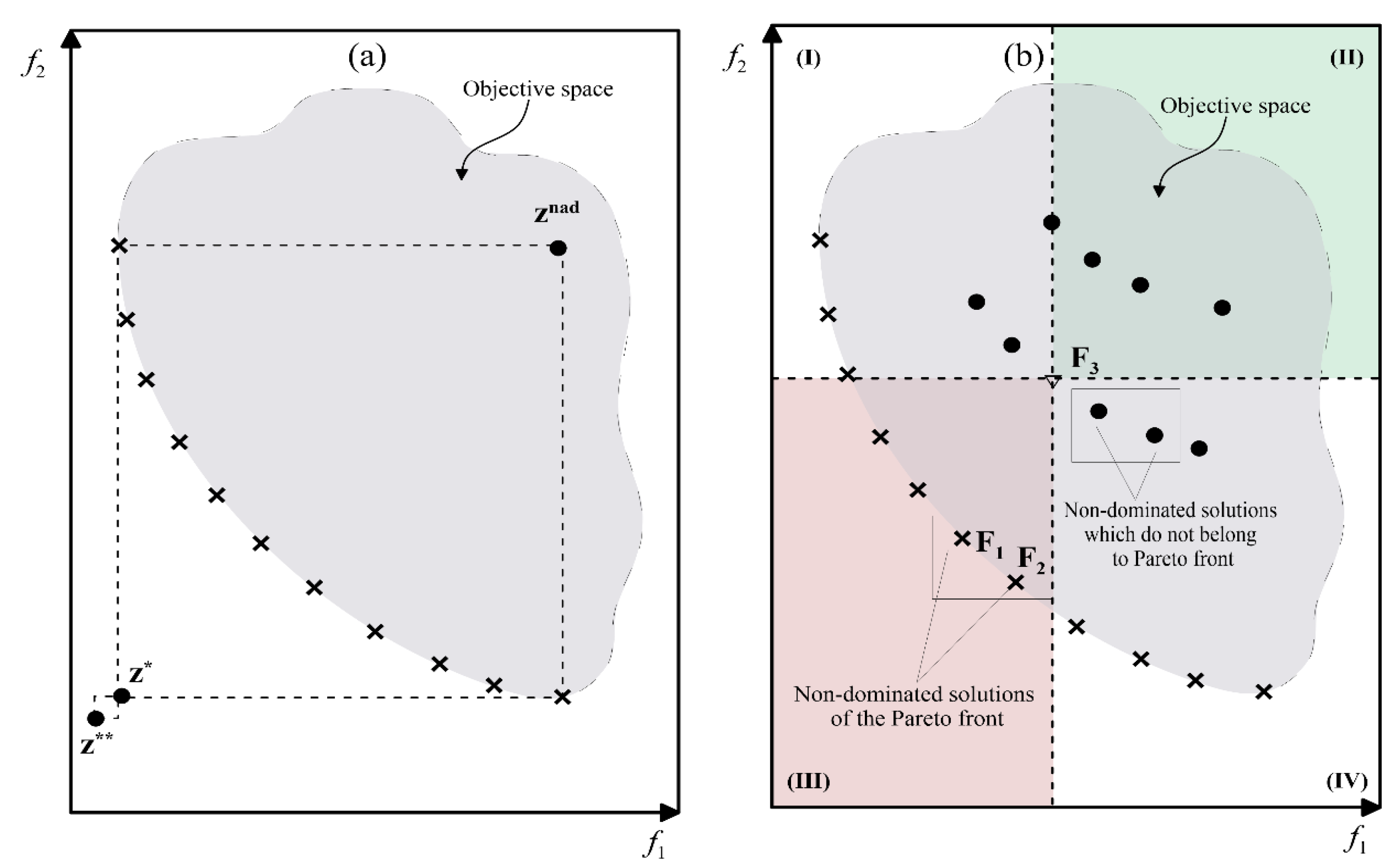
2.3.1. The Optimum in MOP

The notion of minimum in relation to the MOP (Equation (10)), differs from Equation (1) for the mono-objective case. Due to the conflict between the elements of the objective-vector, there is no single solution to the minimization problem. Hence, the ordering of the possible solutions of the MOP is partial [17], so that:

Definition 0

OF₁ = OF(θ₁) = {s_m¹}_m^M is less than OF₂ = OF(θ₂) = {s_m²}_m^M, (OF₁ < OF₂) if and only if: s_m¹ ≤ s_m² for any value of “m.”

An optimal solution of the MOP, θ^*, will not allow the existence of another θ, where the above condition is verified. This idea of optimality, generalized by Vilfredo Pareto [37], is formalized as follows:

Definition 1

(dominance relationship). It is said that one parametrization θ₁ dominates another θ₂, denoted by θ₁ ≤ θ₂, if the following expression is verified:

$${\mathsf{\theta }}_1\underset{\_}{\prec }{\mathsf{\theta }}_2\iff s_{\mathrm{m}}^1\le s_{\mathrm{m}}^2\forall \mathrm{m}\in [1,M]\wedge \exists \mathrm{m}/s_{\mathrm{m}}^1<s_{\mathrm{m}}^2$$

(11)

a non-dominated solution is also called an efficient solution [38,39].

Definition 2

(global optimum in the Pareto sense). A global optimum in the sense of Pareto is a solution for which there is no other solution belonging to the feasible space Ω to dominate it.

$${\mathsf{\theta }}^{*}\mathrm{is} \mathrm{the} \mathrm{Pareto} \mathrm{optimum} \hspace{0.17em}\iff !\exists \mathsf{\theta }\in \Omega /\mathsf{\theta }\underset{\_}{\prec }{\mathsf{\theta }}^{*}$$

(12)

Definition 3

(Pareto or efficient set). The efficient set is composed of the global optima of the MOP.

$${\mathcal{P}}^{*}=\left\{{\mathsf{\theta }}^{*}\in \Omega \backslash !\exists \mathsf{\theta }\in \Omega :\mathsf{\theta }\underset{\_}{\prec }{\mathsf{\theta }}^{*}\right\}$$

(13)

Definition 4

(Pareto front or efficient front). The expression of the efficient set in the region of the objective functions of the problem makes up the efficient front.

$$P{F}^{*}=\left\{FO(\mathsf{\theta })/\mathsf{\theta }\in P^{*}\right\}$$

(14)

In most cases it is not possible, even computationally, to obtain an analytical expression that defines the PF^*. Therefore, methods to solve the MOP attempt to approximate this set by sampling. This gives an approximation of the efficient front, as illustrated in Figure 6a. This leads to the dominance relationships shown in Figure 6b.

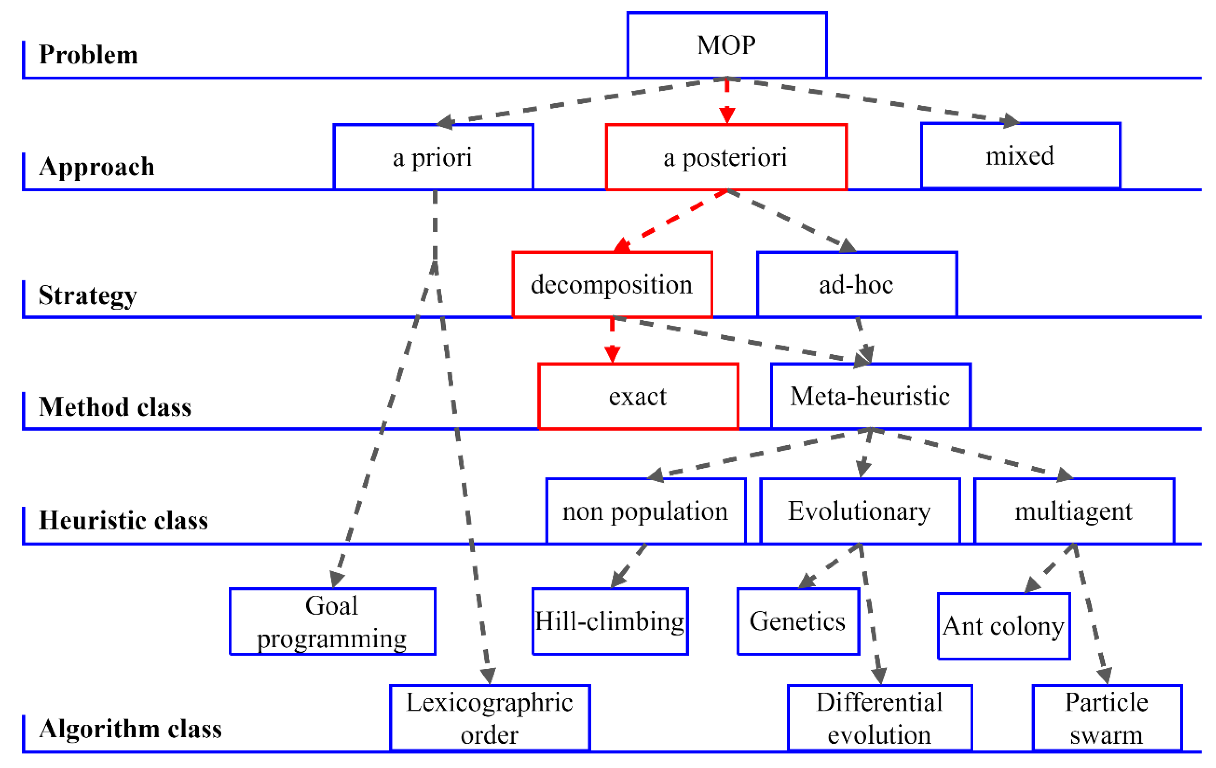
2.3.2. Resolution of the MOP

Equation (10) can be solved in different ways, as depicted in Figure 7, organized in categories from higher to lower specificity, and including procedures taken from the literature [39,40,41,42,43,44,45,46,47].

The first level shows the optimization approaches, highlighting the one qualified as a posteriori that provides a more exhaustive description of the Pareto set of the MOP, whereas the final chosen solution is carried out in a later step depending on the established preferences. The most significant steps in this approach are those of decomposition [41] and ad hoc. The former divides the original MOP into several mono-objective subproblems, whose resolution is addressed by exact methods (branch-and-bound [42] or BARON [43]) and meta-heuristic methods (simulated annealing) [44]. The ad hoc strategy uses a heuristic or meta-heuristic approach that simultaneously addresses a set of candidate solutions for the Pareto set. This requires a population of the heuristic type (evolutionary or multi-agent) [40,45], as shown in the mentioned diagram.

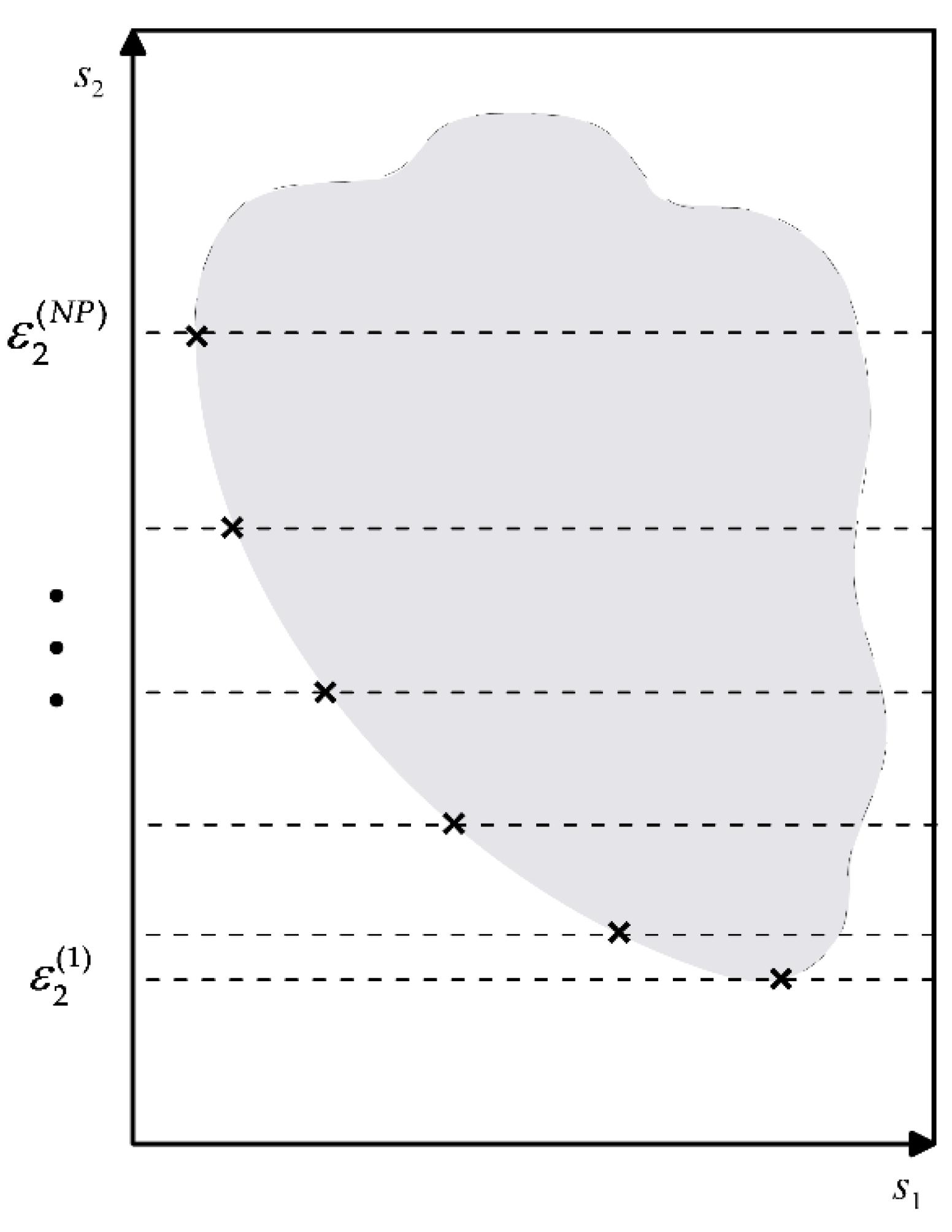
2.3.3. Resolution by ε-Constraint Decomposition

In this work, the parametrization of NRTL by MOP was carried out by ε-constraint decomposition [17,38,39], wherein elements of the OF, except one, are reconverted into constraints of the problem according to the equation given below.

In this way, the multi-objective approach is transformed into a mono-objective problem with inequality constraints that are added to those of the MOP. The ε_m values are upper limits for each objective converted into a constraint, so that the Pareto set is constructed using a grid of ε_m values over which each particular mono-objective problem generated is solved (Figure 8).

$$\begin{array}{l}\underset{\mathsf{\theta }}{\min }{s}_{\mathrm{ELL}}(\mathsf{\theta }|Y^{\exp },x^{\exp })\\ \mathrm{s}.\mathrm{t}. A\mathsf{\theta }\le b\\ \hspace{0.17em}\hspace{0.17em}\hspace{0.17em}\hspace{0.17em}\hspace{0.17em}\hspace{0.17em}\hspace{0.17em}\hspace{0.17em}\hspace{0.17em}g(\mathsf{\theta }|Y^{\exp },x^{\exp })\le 0\\ \hspace{0.17em}\hspace{0.17em}\hspace{0.17em}\hspace{0.17em}\hspace{0.17em}\hspace{0.17em}\hspace{0.17em}\hspace{0.17em}\hspace{0.17em}h(\mathsf{\theta }|Y^{\exp },x^{\exp })=0\\ \hspace{0.17em}\hspace{0.17em}\hspace{0.17em}\hspace{0.17em}\hspace{0.17em}\hspace{0.17em}\hspace{0.17em}\hspace{0.17em}\hspace{0.17em}{s}_{\mathrm{ELV}}(\mathsf{\theta }|Y^{\exp },x^{\exp })\le {\epsilon }_{\mathrm{ELV}}\\ \hspace{0.17em}\hspace{0.17em}\hspace{0.17em}\hspace{0.17em}\hspace{0.17em}\hspace{0.17em}\hspace{0.17em}\hspace{0.17em}\hspace{0.17em}{s}_{\mathrm{h}}(\mathsf{\theta }|Y^{\exp },x^{\exp })\le {\epsilon }_{\mathrm{h}}\\ \hspace{0.17em}\hspace{0.17em}\hspace{0.17em}\hspace{0.17em}\hspace{0.17em}\hspace{0.17em}\hspace{0.17em}\hspace{0.17em}\hspace{0.17em}\mathsf{\theta }\in P\hspace{0.17em}\hspace{0.17em}\end{array}$$

(15)

2.3.4. Resolution of the Multi-Property Problem as an MOP

The modelling was solved using Equation (10), taking into account Equation (15) and the statistical parameters shown in Section 2. In the ε-constraint decomposition, the LLE error was adopted as the objective function, whereas the model errors in the VLE representation and the h^Es were formulated as constraints of the problem. A 2D-grid of 8 steps of ε was then defined for the VLE errors in the interval [0.3–0.03] and of 7 steps for h^E/RT in the interval [0.12–0.018]. That is, 56 mono-objective subproblems arose from the decomposition, and each step was solved by the augmented lagrangian method to address problems with constraints. The SLSQP method [46] was selected as a local solver to solve the augmented problem, using the implementation existing in the NLOPT library [47].

2.3.5. Multi-Objective Modelling Using NRTL

The efficient front (Equation (14)), achieved in the non-dominated parametrizations of the NRTL model is represented in Figure 9.

The distribution of solutions shows that the LLE description competed with that of VLE; there were improvements in the LLE and the description of VLE worsened. On the other hand, for a constant error in the VLE description, the s(LLE) statistic did not have the same sensitivity compared to s(h^E). Four different parametrizations (P1–P4) were selected from the front, and their assessments are summarized in

Table 3. Parametrizations of the NRTL using the MOP to model the methyl methanoate (1) + pentane (2) system.

	${\mathit{\tau }}_{\mathbf{ij}/\mathbf{ji}}^{(0)}$	${\mathit{\tau }}_{\mathbf{ij}/\mathbf{ji}}^{(1)}$	${\mathit{\tau }}_{\mathbf{ij}/\mathbf{ji}}^{(2)}$	${\mathit{\tau }}_{\mathbf{ij}/\mathbf{ji}}^{(3)}$	${\mathit{\alpha }}_{21}$
P1	20.000/18.845	2376.45/1879.56	−7.817/−6.099	0.0691/0.0247	0.0308
P2	12.746/24.428	2379.16/1882.88	−8.113/−6.249	0.1145/−0.0038	0.0144
P3	34.675/30.078	2377.47/1880.99	−10.000/−10.000	0.1381/−0.0095	0.0027
P4	30.764/31.139	2377.50/1881.07	−9.999/−9.445	0.1325/−0.0053	0.0041
		s(LLE)	s(ELV)	s(hE/RT)
	P1	0.0137	0.2995	0.0203
	P2	0.0338	0.0310	0.0175
	P3	0.0201	0.1079	0.0860
	P4	0.0220	0.1079	0.0180

and the representations compared in Figure 9.

The graphical/numerical analysis of Figure 9 shows that the parametrization P2 acceptably represents the T vs x, or y curves of the VLE (see Figure 10a), those of γ_is and the g^E/RT (Figure 10b), and that of the h^Es, (Figure 10d). However, quantitatively it did not represent the LLE well, with an error in the UCST of ΔT_UCST ≈ 11 K, lower than that obtained with the multi-property mono-objective approach.

The theoretical limitations of NRTL can be seen by comparing the estimations made with the different parametrizations. Thus, P1, P2, and P4 better reflected the functional g^E = ϕ(T) and, therefore, provided a better description of the h^Es; the parametrizations P1 and P3 acceptably described the LLE and P2 represented the VLE well, including the azeotropes, both qualitatively and quantitatively.

2.4. Comments on the Strategies of Analyzed Modelling

The results obtained by solving the MOP (Table 3) are represented in terms of the g^E function in Figure 11. The modelling in Figure 11a is the one that best describes the LLE (see Figure 10c) since the surface of g^E had a morphology similar to that produced by the conventional parametrization procedure (Section 2.1). The difference between the two is due to the fact that the inclusion of VLE and h^E data controlled the slope around the immiscibility region, preventing it from evolving to negative g^E values (see Figure 4).

The situation that best describes the VLE (P2) is shown in Figure 11b, showing higher g^E values around the vapor–liquid coexistence region, causing increases in the temperature interval where two liquid phases coexist (unlike the experimental behavior). Figure 11c,d, illustrates the importance of including the h^Es in the model definition. The NRTL equation tended to generate negative slopes of g^E close to the immiscibility region, producing a minimum on the surface (Figure 4) when the h^Es were not considered (Figure 3c). By contrast, this slope on the surface was not as steep (Figure 11d). In summary, the inclusion of the h^Es is relevant to improving the extrapolation with the model thus obtained.

3. Influence of Modelling on the Simulation of a Separation Process

The impact of the strategy that has been carried out on the modelling in chemical engineering calculations was analyzed by applying the results obtained in the previous section to a simulation process to separate pentane and methyl methanoate from a binary solution, an azeotropic solution chosen because it cannot be completely separated by simple rectification. Several methods can be used to carry out this operation [48], such as extractive distillation or a pressure swing. Moreover, as the chosen binary presents two immiscible liquid phases at T < 260 K, the separation was proposed by combining the aforementioned distillation and simple decantation. The simulation experiences discussed here were performed using Aspen Plus© software using the Radfrac calculator block for the rectification columns.

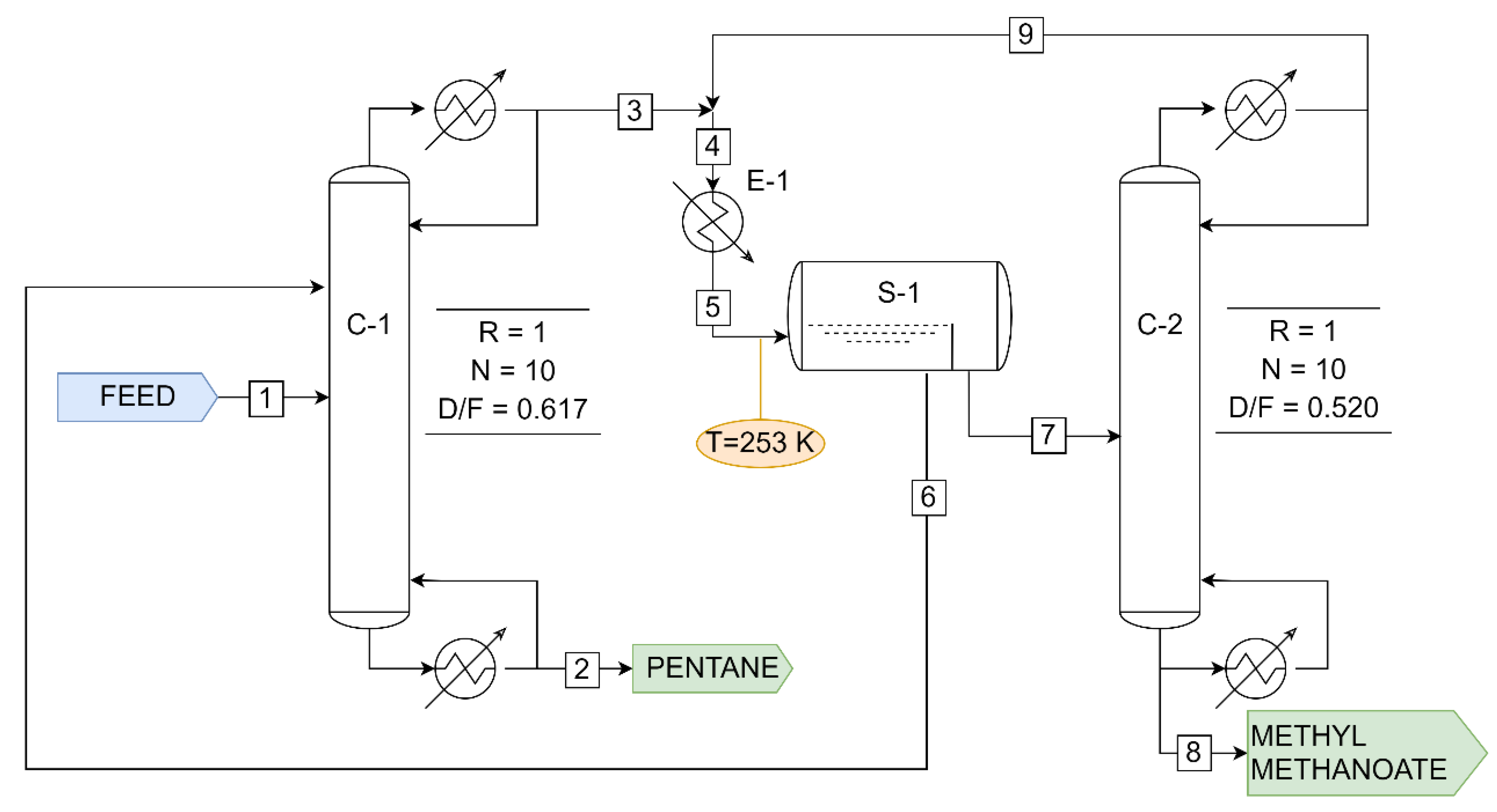
3.1. Description of the Separation Process

The flow diagram of the process followed is shown in Figure 12. It was designed to treat 1000 kmol⋅h⁻¹ of the binary methyl methanoate (1) + pentane (2) (at ambient conditions), with an initial molar composition in ester of 30% (<x_az ≈ 0.56).

The identification of each stream/operation is indicated:

-

Distillation column C-1: recovery of pentane in bottom streams;

-

Distillate, stream 3: product under conditions close to azeotrope;

-

Distillates of C-1 and C-2 (x₁ ≈ x_az) are blended and sent to E-1;

-

E-1 exchanger cools to form two immiscible liquid phases;

-

Decanter S-1 separates the immiscible liquid phases;

-

Stream 5 (x₁ < x_az) is recirculated to column C-1;

-

Stream 6 (x₁ > x_az) feeds column C-2;

-

The ester is obtained by the C-2 bottom.

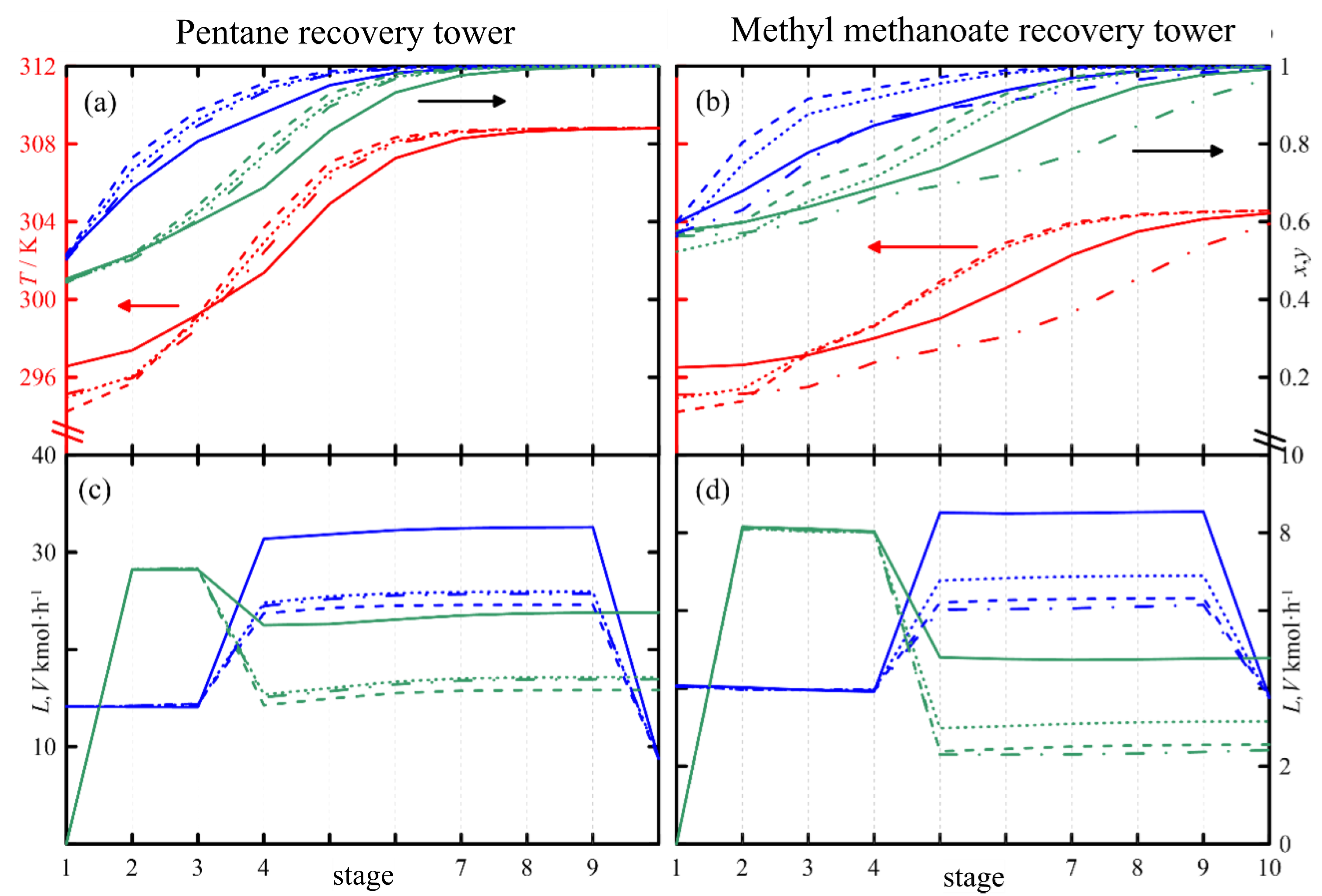
3.2. Results of the Simulation

The behavior of C-1 estimated by the results P2, P3, and P4 of the model was similar, although the case P1 produced a smaller profile of compositions and higher temperatures at the head of the column and smaller ones at the bottom (Figure 13a) compared with the other simulation results. This is because P1 described the VLE the worst (Figure 10a). However, in C-2 (Figure 13b), only P2 and P4 produced similar results. P3 showed smaller values than when the modelling was used with the other parametrizations, both in the compositions and in the temperature of most of the stages. This was not due to differences in the description of the VLE, since the results of P3 and P4 were very similar in this diagram, but because P3 estimated a greater amount of pentane in phase-I at T = 253 K (Figure 10c), generating more methyl methanoate in the feed of C-2 (since the separation in S-1 is worse), which affected the material and energy balances. In fact, when the process was simulated with P3, stream 7 had about 2% more ester than when P4 was used. On the other hand, the result obtained with P1 showed similar discrepancies to those of C-1. Moreover, P1 produced the greatest discrepancies in terms of molar flow (Figure 13c,d) in both columns.

The discussion presented shows that different behaviors that are generated depending on the parametrization used have a significant impact on the simulation/design of the process.

4. Conclusions

The NRTL model used in this work (Equations (A-10) and (A-12)) has theoretical limitations that are compensated for using several adjustable parameters established with experimental data (VLE, LLE, h^E) obtained from the real behavior of the solutions. Experimental information of the system methyl methanoate + pentane was processed to define the set of parameters of NRTL that show the best representation of the different properties of this mixture. That is, the strategy adopted for the parametrization conditions its validity.

The conventional approach to modelling problems with LLE and/or VLE data only provides local descriptions of the system behavior, since the Gibbs function (and the corresponding g^E) cannot be characterized over a wide range of conditions from a limited number of observations (see Figure 4).

Employing a multi-property approach allows the validity of the set of parameters to be extended without excessively increasing the experimental database. However, this approach is not sufficient when the level of theory, or the flexibility of the correlations employed, cannot be described over the entire range observed. In these cases, the application of Equations (2) or (3) does not ensure that the set of parameters obtained is optimal. Hence, in this work the parametrization problem is addressed by means of multi-objective optimization (MOP), considering that it is more convenient. The methodology used systematically identifies optimal (non-dominated) parametrizations, each of which provides a more precise local description of the quantities that configure the overall behavior of the system (see Figure 10).

Comparison of four parametrizations (P1 to P4) representative of the optimal set (Table 3) revealed that the profiles of composition, temperature, and molar flow inside the rectification columns C-1 and C-2 are conditioned by the parametrization used, which ultimately affects the results of the process. The MOP approach establishes several optimal alternatives, and the process engineer should select the one that provides a suitable technical/economic solution to achieve the proposed objective. The methodology applied in this work to a specific case, selected by the availability of experimental quantities of several properties, is very useful, but it cannot be generalized for all types of solutions; on the contrary, it must be verified for each case. Logically, the application of this methodology is simplified when the number of properties in the modelling process decreases. On the other hand, its extension to multicomponent systems is more complex (especially with the presence of LLE data) and it is the objective of future works.

References

1. Smith, J.M.; Van Ness, H.C.; Abbott, M.M. Introduction to Chemical Engineering Thermodynamics, 7th ed.; McGraw-Hill: Boston, MA, USA, 2005. [Google Scholar]
2. Wankat, P.C. Separations Process Engineering: Includes Mass Transfer Analysis, 3rd ed.; Prentice Hall: Boston, MA, USA, 2012. [Google Scholar]
3. Prausnitz, J.M.; Lichtenthaler, R.N.; de Azevedo, E.G. Molecular Thermodynamics of Fluid-Phase Equilibria; Prentice Hall PTR: Upper Saddle River, NJ, USA, 1999. [Google Scholar]
4. Ortega, J.; Espiau, F.; Wisniak, J. New parametric model to correlate the Gibbs excess function and other thermodynamic properties of multicomponent systems. Application to binary systems. Ind. Eng. Chem. Res. 2010, 49, 406–421. [Google Scholar] [CrossRef]
5. Renon, H.; Prausnitz, J.M. Local compositions in thermodynamic excess functions for liquid mixtures. AIChE J. 1968, 14, 135–144. [Google Scholar] [CrossRef]
6. Abrams, D.S.; Prausnitz, J.M. Statistical thermodynamics of liquid mixtures: A new expression for the excess Gibbs energy of partly or completely miscible systems. AIChE J. 1975, 21, 116–128. [Google Scholar] [CrossRef]
7. Peng, D.-Y.; Robinson, D.B. A New Two-Constant Equation of State. Ind. Eng. Chem. Fundam. 1976, 15, 59–64. [Google Scholar] [CrossRef]
8. Soave, G. Equilibrium constants from a modified Redlich-Kwong equation of state. Chem. Eng. Sci. 1972, 27, 1197–1203. [Google Scholar] [CrossRef]
9. Valderrama, J.O. The state of the cubic equations of state. Ind. Eng. Chem. Res. 2003, 42, 1603–1618. [Google Scholar] [CrossRef]
10. Klamt, A.; Schüürmann, G. COSMO: A new approach to dielectric screening in solvents with explicit expressions for the screening energy and its gradient. J. Chem. Soc. Perkin Trans. 1993, 2, 799–805. [Google Scholar] [CrossRef]
11. Klamt, A. Conductor-like Screening Model for Real Solvents: A new approach to the quantitative calculation of solvation phenomena. J. Phys. Chem. 1995, 99, 2224–2235. [Google Scholar] [CrossRef]
12. Lin, S.-T.; Sandler, S.I. A priori phase equilibrium prediction from a segment contribution solvation model. Ind. Eng. Chem. Res. 2002, 41, 899–913. [Google Scholar] [CrossRef]
13. Chapman, W.G.; Gubbins, K.E.; Jackson, G.; Radosz, M. SAFT: Equation-of-state solution model for associating fluids. Fluid Phase Equilib. 1989, 52, 31–38. [Google Scholar] [CrossRef]
14. Gross, J.; Sadowski, G. Perturbed-Chain SAFT: An Equation of State Based on a Perturbation Theory for Chain Molecules. Ind. Eng. Chem. Res. 2001, 40, 1244–1260. [Google Scholar] [CrossRef]
15. Gross, J.; Sadowski, G. Application of the Perturbed-Chain SAFT Equation of State to Associating Systems. Ind. Eng. Chem. Res. 2002, 41, 5510–5515. [Google Scholar] [CrossRef]
16. Fredenslund, A.; Jones, R.L.; Prausnitz, J.M. Group-contribution estimation of activity coefficients in nonideal liquid mixtures. AIChE J. 1975, 21, 1086–1099. [Google Scholar] [CrossRef]
17. Miettinen, K. Nonlinear Multiobjective Optimization; Springer: Boston, MA, USA, 1998. [Google Scholar] [CrossRef]
18. Pérez-Fortes, M.; Schöneberger, J.C.; Boulamanti, A.; Tzimas, E. Methanol synthesis using captured CO2 as raw material: Techno-economic and environmental assessment. Appl. Energy 2016, 161, 718–732. [Google Scholar] [CrossRef]
19. Forte, E.; Burger, J.; Langenbach, K.; Hasse, H.; Bortz, M. Multi-criteria optimization for parameterization of SAFT-type equations of state for water. AIChE J. 2018, 64, 226–237. [Google Scholar] [CrossRef]
20. Sosa, A.; Fernández, L.; Gómez, E.; Macedo, E.A.; Ortega, J. A practical fitting method involving a trade-off decision in the parametrization procedure of a thermodynamic model and its repercussion on distillation processes. In Distillation—Modeling, Simulation and Optimization; Steffen, V., Ed.; IntechOpen: London, UK, 2019. [Google Scholar] [CrossRef]
21. Sosa, A.; Fernández, L.; Ortega, J.; Jiménez, L. The parametrization problem in the modeling of the thermodynamic behavior of solutions. An approach based on information theory fundamentals. Ind. Eng. Chem. Res. 2019, 58, 12876–12893. [Google Scholar] [CrossRef]
22. Lee, Y.S.; Graham, E.J.; Galindo, A.; Jackson, G.; Adjiman, C.S. A comparative study of multi-objective optimization methodologies for molecular and process design. Comput. Chem. Eng. 2020, 136, 106802. [Google Scholar] [CrossRef]
23. Forte, E.; Kulkarni, A.; Burger, J.; Bortz, M.; Küfer, K.-H.; Hasse, H. Multi-criteria optimization for parametrizing excess Gibbs energy models. Fluid Phase Equilib. 2020, 522, 112676. [Google Scholar] [CrossRef]
24. Franzosini, P.; Geangu-Moisin, A.; Ferloni, P. Some Remarks on methylformate + n-alkanes Binary Systems. Z. Naturforsch. A 1970, 25, 457–458. [Google Scholar] [CrossRef]
25. Fernández, F.; Ortega, J.; Sabater, G.; Espiau, F. Experimentation and thermodynamic representations of binaries containing compounds of low boiling points: Pentane and alkyl methanoates. Fluid Phase Equilib. 2014, 363, 167–179. [Google Scholar] [CrossRef]
26. Gmehling, J.; Onken, U.; Rarey-Nies, J.R.; Arlt, W.; Weidlich, U.; Grenzheuser, P.; Kolbe, B. Vapor-liquid Equilibrium Data Collection DECHEMA Chemistry Data Series; DECHEMA: Frankfurt, Germany, 1977; Volume 1–8. [Google Scholar]
27. Marina, J.M.; Tassios, D.P. Effective local compositions in phase equilibrium correlations. Ind. Eng. Chem. Process. Des. Dev. 1973, 12, 67–71. [Google Scholar] [CrossRef]
28. Fredenslund, A.A.; Gmehling, J.; Rasmussen, P. Vapor-Liquid Equilibria Using UNIFAC. A Group-Contribution Method; Elsevier: Amsterdam, The Netherlands, 1977. [Google Scholar]
29. Britt, H.I.; Luecke, R.H. The estimation of parameters in nonlinear, implicit models. Technometrics 1973, 15, 233–247. [Google Scholar] [CrossRef]
30. Anderson, T.F.; Abrams, D.S.; Grens, E.A. Evaluation of parameters for nonlinear thermodynamic models. AIChE J. 1978, 24, 20–29. [Google Scholar] [CrossRef]
31. Ortega, J.; Espiau, F. A new correlation method for vapor−liquid equilibria and excess enthalpies for nonideal solutions using a genetic algorithm. Application to ethanol+an n-alkane mixtures. Ind. Eng. Chem. Res. 2003, 42, 4978–4992. [Google Scholar] [CrossRef]
32. Fernández, L.; Ortega, J.; Pérez, E.; Toledo, F.J.; Canosa, J. multiproperty correlation of experimental data of the binaries propyl ethanoate + alkanes (pentane to decane). New experimental information for vapor–liquid equilibrium and mixing properties. J. Chem. Eng. Data 2013, 58, 686–706. [Google Scholar] [CrossRef]
33. Espiau, F.; Ortega, J.; Penco, E.; Wisniak, J. Advances in the correlation of thermodynamic properties of binary systems applied to methanol mixtures with butyl esters. Ind. Eng. Chem. Res. 2010, 49, 9548–9558. [Google Scholar] [CrossRef]
34. Ríos, R.; Ortega, J.; Sosa, A.; Fernández, L. Strategy for the management of thermodynamic data with application to practical cases of systems formed by esters and alkanes through experimental information, checking-modeling, and simulation. Ind. Eng. Chem. Res. 2018, 57, 3410–3429. [Google Scholar] [CrossRef]
35. Espiau, F.; Ortega, J.; Fernández, L.; Wisniak, J. Liquid–liquid equilibria in binary solutions formed by [pyridinium-derived][F4 B] ionic liquids and alkanols: New experimental data and validation of a multiparametric model for correlating LLE data. Ind. Eng. Chem. Res. 2011, 50, 12259–12270. [Google Scholar] [CrossRef] [Green Version]
36. Ko, M.; Im, J.; Sung, J.Y.; Kim, H. Liquid-liquid equilibria for the binary systems of sulfolane with alkanes. J. Chem. Eng. Data 2007, 52, 1464–1467. [Google Scholar] [CrossRef]
37. Pareto, V. Cours d’économie Politique; Librairie Droz: Geneva, Switzerland, 1964. [Google Scholar]
38. Mavrotas, G. Effective implementation of the e-constraint method in Multi-Objective Mathematical Programming problems. Appl. Math. Comput. 2009, 213, 455–465. [Google Scholar] [CrossRef]
39. Deb, K. Multi-Objective Optimization Using Evolutionary Algorithms; John Wiley & Sons: Chichester, UK, 2001. [Google Scholar]
40. Coello, C.; Lamont, G.; Van Veldhuisen, D. Evolutionary Algorithms for Solving Multi-Objective Problems; Springer: Boston, MA, USA, 2007. [Google Scholar] [CrossRef]
41. Zhang, Q.; Li, H. MOEA/D: A multiobjective evolutionary algorithm based on decomposition. IEEE Trans. Evol. Comput. 2007, 11, 712–731. [Google Scholar] [CrossRef]
42. Belotti, P.; Kirches, C.; Leyffer, S.; Linderoth, J.; Luedtke, J.; Mahajan, A. Mixed-integer nonlinear optimization. Acta Numer. 2013, 22, 1–131. [Google Scholar] [CrossRef]
43. Sahinidis, N.V. BARON: A general purpose global optimization software package. J. Glob. Optim. 1996, 8, 201–205. [Google Scholar] [CrossRef]
44. Černý, V. Thermodynamical approach to the traveling salesman problem: An efficient simulation algorithm. J. Optim. Theory Appl. 1985, 45, 41–51. [Google Scholar] [CrossRef]
45. Mishra, D.K.; Shinde, V. A review of global optimization problems using meta-heuristic algorithm. In Nature-Inspired Optim. Algorithms; Khamparia, A., Khanna, A., Bao Le, N., Nhu Gia, N., Eds.; De Gruyter: Berlin, Germany, 2021; pp. 87–106. [Google Scholar] [CrossRef]
46. Kraft, D. Algorithm 733; TOMP-Fortran modules for optimal control calculations. ACM Trans. Math. Softw. 1994, 20, 262–281. [Google Scholar] [CrossRef]
47. Johnson, S.G. The NLopt Nonlinear-Optimization Package, Version 2.6.1; GitHub: San Francisco, CA, USA, 2019. [Google Scholar]
48. Seader, J.D.; Henley, E.J. Separation Process Principles, 2nd ed.; Wiley: Hoboken, NJ, USA, 2006. [Google Scholar]
Figure 1. Distillation, an example of a unitary operation raised as a succession of equilibrium stages. Each stage is considered a VLE state, and all make up a distillation column.
Thermo 02 00019 g001
Figure 2. Diagram representing different options to optimize the parameterization of a thermodynamic model.
Thermo 02 00019 g002
Figure 3. Estimations obtained with the NRTL model using experimental data for the binary methyl methanoate (1) + pentane (2). The classical approach () APV88 for (a) LLE, T v s x 1 I , or x 1 II ; (b) VLE, T vs x1, or y1; (c) hEvs x1. ◇, experimental data.
Thermo 02 00019 g003
Figure 4. Plot of gE = gE(p,T,x) using the NRTL model and the APV88 parametrization. Projection on the T vs x1 plane corresponding to the geometric place of the LLE compositions is included.
Thermo 02 00019 g004
Figure 5. Plot of the estimations obtained for (a) T v s x 1 I , or x 1 II (LLE), (b) T va x1, or y1 (VLE), (c) hE vs x1, using two parametrizations of the NRTL model for the binary methyl methanoate (1) + pentane (2). (– –) ref [25]; () APV88. ◇, experimental data.
Thermo 02 00019 g005
Figure 6. Description of the objective space of the MOP. (a) Objective space and Pareto front; (b) division of objective space according to dominance relationships, (I) and (IV) regions with non-dominated solutions that do not dominate by OF3, (II) region of solutions dominated by OF3, (III) solutions that dominate OF3.
Thermo 02 00019 g006
Figure 7. Approximations to solve the MOP. In red, the route proposed in this work.
Thermo 02 00019 g007
Figure 8. Construction of the efficient front applying the ε-constraint method. The front points are obtained by solving each restricted mono-objective subproblem (Equation (15)).
Thermo 02 00019 g008
Figure 9. Two different views (a,b) according to the arrows of the efficient front obtained with the ε-constraint methodology. Selected parametrizations for the NRTL model: (P1) ; (P2) ✕; (P3) ; (P4) .
Thermo 02 00019 g009
Figure 10. Estimation diagrams by NRTL using the indicated parametrizations: (a) VLE: T vs x1, or y1; (b) γi or gE/RT vs x1; (c) LLE: T v s x 1 I , or x 1 II ; (d) hE vs x1.
Thermo 02 00019 g010
Figure 11. Plot of gE vs x1, or T using NRTL with the parametrizations of Table 3. (a) P1; (b) P2; (c) P3; (d) P4. (). Geometric space of gE for the two phases VLE and LLE.
Thermo 02 00019 g011
Figure 12. Flow diagram of the separation process of the binary methyl methanoate (1) + pentane (2). R = reflux ratio; D/F = distillate/feed ratio; N = number of stages.
Thermo 02 00019 g012
Figure 13. Profiles in the recovery columns of pentane (C-1) and methyl methanoate (C-2). (a,b) (▪▪▪▪) temperature; (▪▪▪▪▪▪▪) liquid composition (▪▪▪▪▪▪▪) vapor composition. (c,d) (▪▪▪▪▪▪▪); liquid flow, L (▪▪▪▪▪▪▪▪) vapor flow, V. (—) P1, (– – –) P2, (– ⋅ –⋅ –) P3, (· · · ·) P4.
Thermo 02 00019 g013