1. Introduction
Yesterday’s vision of in-space manufacturing will become tomorrow’s reality [
1]. This statement, made in 1993, finds its confirmation today when NASA seeks a paradigm shift in the design and manufacturing of space architectures to enable the on-demand fabrication of critical systems. In particular, the In-Space Manufacturing (ISM) project at NASA’s Marshall Space Flight Center, in collaboration with industrial partners, is developing capabilities for the 3D additive manufacturing (AM) of metals in space. Research aimed at supporting 3D printing capabilities in space was reported earlier [
2,
3].
Here the technology of bound metal deposition (BMD) is analysed. BMD is currently being matured for International Space Station experiments. It is an extrusion-based process of additive manufacturing, sometimes referred to as shaping, debinding, sintering (SDS) [
4]. In this process, metal powder—particles of micron size—are mixed with a soft binder that keeps the mixture together. During the shaping stage the mixture is usually heated to soften the binder and then dispensed through a nozzle. The exact toolpaths and extrusion rates are calculated to shape the required geometry of the part, which is called “green” at this stage.
The shaping step is followed by placing the part in the debinder and removing the binder from it. Up to 70% of the primary binder can be sometimes removed by chemical dissolution or thermal debinding, while the remaining binder helps the part to retain its shape. The main point of interest here lies in the debinding achieved by thermal decomposition, after which the part is called “brown”.
Finally, densified metallic components are obtained through sintering. Densification occurs in two steps. First, there is necking of the powder particles [
5,
6,
7]. At the next stage, sintering occurs via diffusion of vacancies along grain boundaries and free surfaces from the interior to the external surface of the sample [
8,
9,
10]. Final densities can reach up to 96–99.8% of theoretical values, depending on the processing characteristics, while the part will shrink by up to 13–25%. The challenges of the latter process include possible defects in the microstructure, reduced density, residual stress, cracking, and nonlinear shrinkage of the final parts. For example, experimentally observed [
11] shrinkage in the vertical direction can be as high as 25%, exceeding that in the horizontal plane by 10%. Several factors affect BMD including the particle size distribution, the packing and filling densities, the geometry of the part, gravity, the debinding process, pressure, and the temperature protocol, to mention a few.
The mechanical properties of the final part are related to the physical properties of the individual metal particles, the bulk properties of the paste, and the processing characteristics. The complexities of these multifaceted relationships [
12] and of the underlying physics render modelling BMD a challenging multi-scale problem. It involves atomic diffusion at the particle–particle interface on the nanoscale [
6,
13,
14], microstructure evolution on the microscale [
14,
15,
16], initial shrinkage and densification of small printed parts with particle resolution on the mesoscale [
17,
18,
19,
20], and macroscopic modelling of the sintering of the whole part [
21,
22,
23].
The difficulties are exacerbated by the fact that the analysis of each physical scale requires a different approach. Thus atomic diffusion is analysed using molecular dynamics (MD) [
13] applied to a few particles. Simulations of the evolution of the microstructure are performed using phase-field methods [
14,
15,
16] for tens of particles. Mesoscale dynamics is simulated by applying the discrete element modelling approach [
17,
18,
19,
20] to the tens of thousands of particles shaping a small submodel of the whole part, while macroscopic analysis is performed using the finite element method [
21,
22,
23] applied to a continuous model of the whole part.
The importance of a multiscale approach to the modelling of sintering was well recognised in both earlier experimental [
24] and numerical [
19,
25,
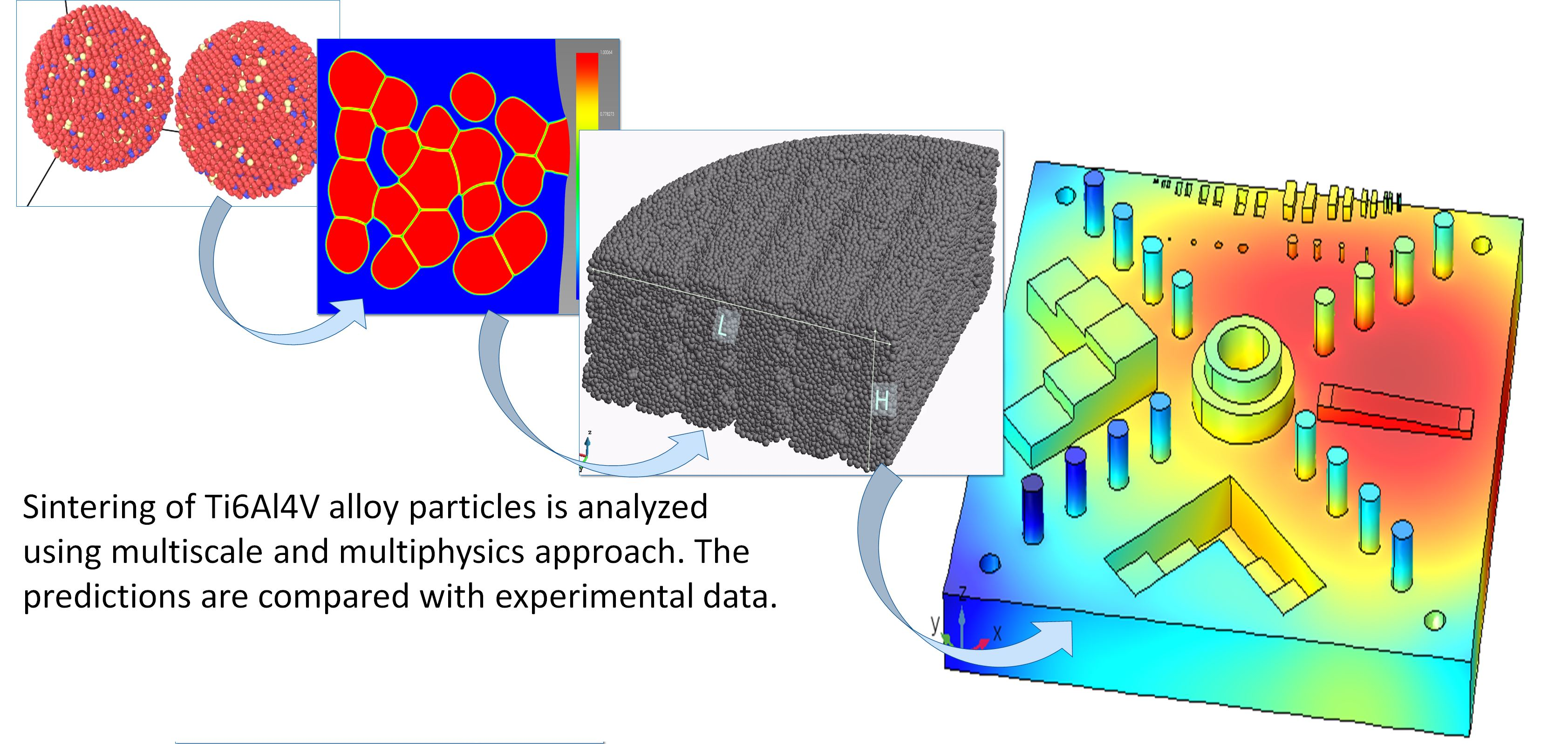
26] research. However, the number of publications remains limited. Here this approach is extended to encompass five different methods of analysis spanning from atomic simulations to the full-scale finite element modelling of sintering of the whole part. The results of simulations on the ground will be compared with those under microgravity, for some of these methods.
In zero gravity, the problem becomes even more involved because gravity is one of the main sources of the nonlinear shrinkage [
11,
27,
28] that results in shape distortion during sintering on the ground. “The first time someone tries to do sintering in a different gravitational environment beyond Earth, or even microgravity, they may be in for a surprise. There just aren’t enough trials yet to tell us what the outcome could be. Ultimately we have to be empirical, give it a try, and see what happens.” [
29].
To extend the analysis of sintering through all of the important scales, and to understand better the corresponding interdependences, a multi-scale modelling approach has been developed spanning from the atomic scale to the dimensions of the whole part. The numerical methods in this approach include: (i) molecular dynamics using LAMMPS [
30,
31]; (ii) phase-field methods using Multiphysics Object-Oriented Simulation Environment—MOOSE Multiphysics [
32]; (iii) discrete element modelling using KRATOS Multiphysics [
33,
34]; (iv) analysis of experimental correlations; (v) finite element modelling using COMSOL [
35].
All these methods have their own advantages and disadvantages and, in what follows, they will be used to estimate the key parameters of the sintering dynamics on different scales. Importantly, the methods are interconnected, so that parameters estimated on one scale are used as input parameters for the next scale up. The performance of these methods will be estimated, and a multi-scale approach combining their individual strengths will be developed.
The manuscript is organised as follows. Molecular dynamics simulations on the scale of tens of nanometers and a few nanoseconds are discussed in
Section 2. Results of the phase-field modelling of the microstructure evolution in the filament cross-section are considered in
Section 3. The application of discrete element modelling for analysis of the initial shrinkage and particle re-arrangement on the scale of a few millimetres and several minutes is discussed in
Section 4. Analysis of experimental correlations and a simplified model of shrinkage are discussed in
Section 5. Finite element modelling of shrinkage in the green, brown and metal parts is analysed in detail in
Section 6. The results are summarised and discussed, and directions for future work are considered, in
Section 7. Finally, conclusions are drawn in
Section 8.
2. Atomistic Modelling of Sintering Ti-6Al-4V Particles
The smallest scale that allows one to simulate the coalescence of metal particles is that of atoms [
19,
25], ranging from single atoms up to ∼100 nm. This allows one to simulate the sintering of a few particles on a time scale ∼100 ns, study the sintering mechanisms, and estimate important system parameters. At the initial stage of sintering, neck growth can invoke several different diffusion mechanisms [
36] including (i) surface diffusion; (ii) lattice diffusion; (iii) evaporation and condensation from the particle surface; (iv) grain boundary diffusion; (v) lattice diffusion from the grain boundary; (vi) plastic flow.
Of these mechanisms, the dominant two are (i) diffusion at the grain boundary; (ii) diffusion at the surface. The driving force for both is the gradient of the chemical potential [
37,
38]: (i) at the grain boundary
; (ii) at the surface
. Here
is the standard chemical potential of the material,
is the normal stress at the boundary,
is the surface energy,
where
r is the radius of the sphere is the surface curvature, and
is the atomic volume. The positive normal stress on the surface
is tension or, if negatve, compression.
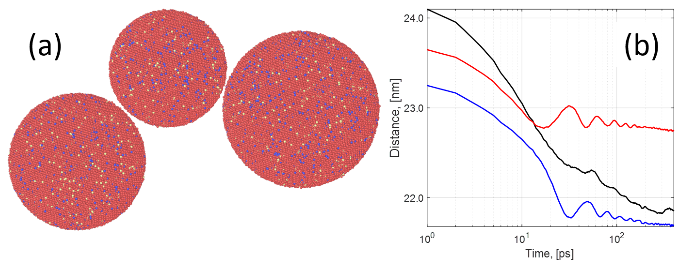
To simulate the sintering of Ti6Al4V nanoparticles, they are first built using the package Atomsk [
39]. An example of the initial configuration of three particles is shown in
Figure 1. The particle diameters are 14 nm for the first particle, 12 nm for the second particle, and 16 nm for the third one. The initial distance between the left and middle particles is ∼14.25 nm and ∼14.65 nm between the middle and right particles. Next, the input files for the LAMMPS package are generated by using Atomsk and then parameters of the modified embedded atom method (MEAM) potentials [
40,
41] are added to these files:
where
F is the embedding energy, which is a function of the atomic electron density
at the position of atom
i,
and is a pair potential interaction, where the parameters
are weight factors and the quantities
with
are partial electron densities,
cohesive energy,
is the background electron density for the reference structure,
A is an adjustable parameter,
is the distance to the
j-th atom from the site
i,
, the decay lengths are adjustable parameters, and
is the nearest-neighbour distance in the equilibrium reference structure. Specific parameters of the MEAM potential used in this work are listed in the
Table 1, see also [
42].
The result of sintering of the three particles in the hcp crystal structure at a temperature
T = 1200 K are shown in
Figure 1b. The initial stage of sintering during the first two picoseconds can be clearly identified in the figure. Particles that are initially separated by a distance of the order 1 nm (edge-to-edge shortest distance) are mutually attracted by the van der Waals force [
44]. Since their initial velocity is zero, the results allow one to estimate the magnitude of the Van der Waals forces. MD simulations also allow one to estimate the number of other important parameters required as inputs to the microscale simulations including diffusion rates and grain boundary width as will now be discussed in more detail.
Analysis of Diffusion
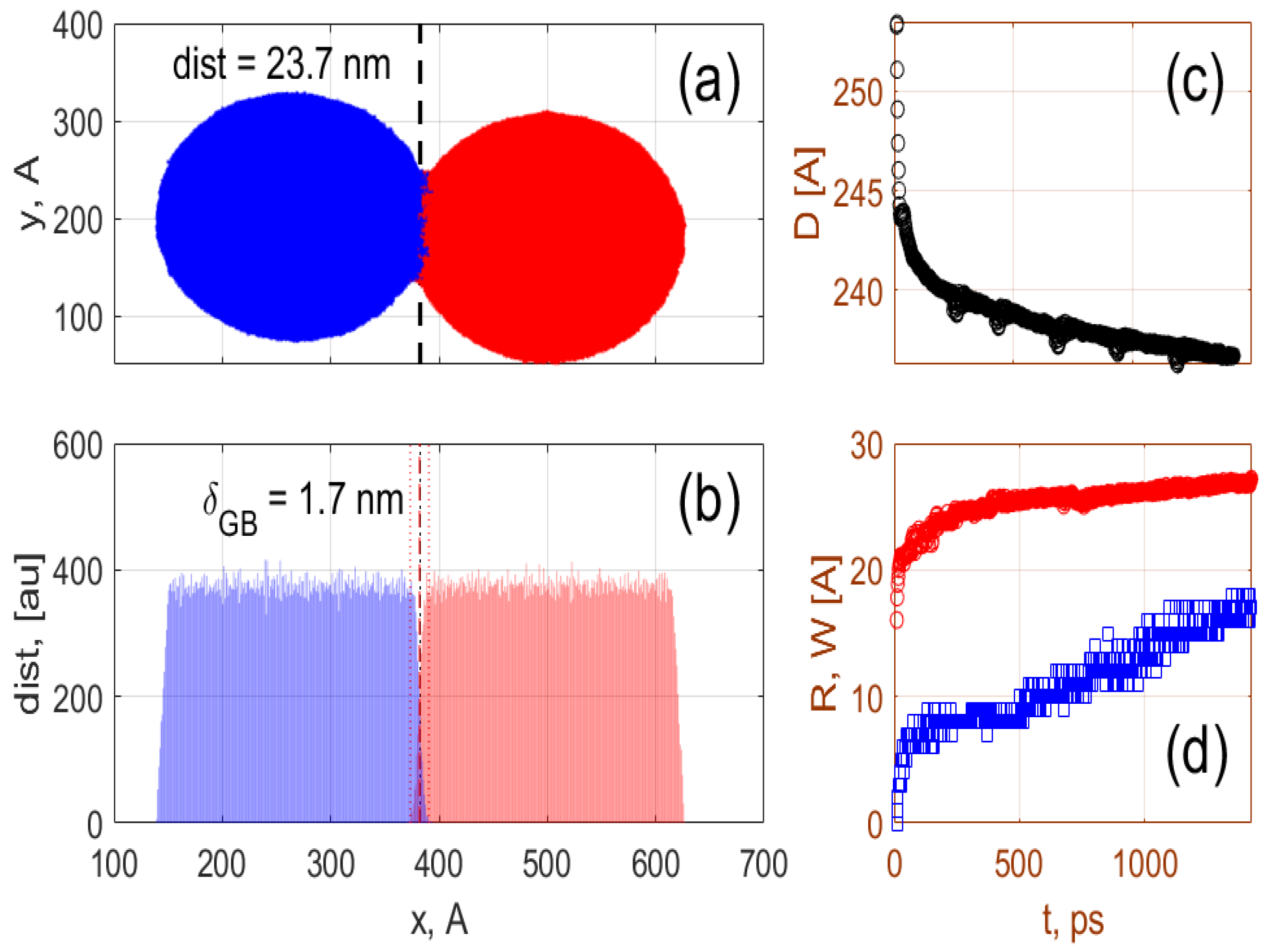
This section describes the analysis of the diffusion of atoms at the interface between two particles with bcc crystal structures, a diameter of 24 nm and a temperature of 1300 K. The results of the simulations are shown in
Figure 2. In the top panel the atoms of the two different particles are shown in blue and pink colours, respectively, and the interface is shown by the vertical dashed line. The distribution of the titanium atoms at the boundary layer after 1 ns of simulation time is shown in
Figure 2 (bottom panel). Following the distribution of atoms in time, one can estimate the distance
D between the particles, the effective width of the boundary layer
, and the radius of the neck
R. The dependences of these parameters on time are shown in the
Figure 2c,d. For example, the distance
between the centres of the particles is shown in the top-right inset of
Figure 2c. It can be seen that the initial fast coalescence of the particles is followed by a steady decrease in
at a rate ≈0.2 nm per ns. This sintering rate corresponds to the growth of the boundary width (≈0.8 nm per ns) and the neck radius (≈0.2 nm per ns). Note that the effective width of the boundary layer defined here is the width of the layer where atoms of both particles are mixed together. It corresponds to the width of the interface layer between the particles that cannot be uniquely attributed to either of these particles. The effective width thus defined can be substantially larger than the width of the boundary layer defined for the atomically clean interface between metal grains [
45]. Experimental evidence of the wider grain boundary can be seen e.g., in the micrograph of a polycrystalline metal obtained in [
46]. The estimated effective grain boundary width (
) will be used for the phase-field modelling.
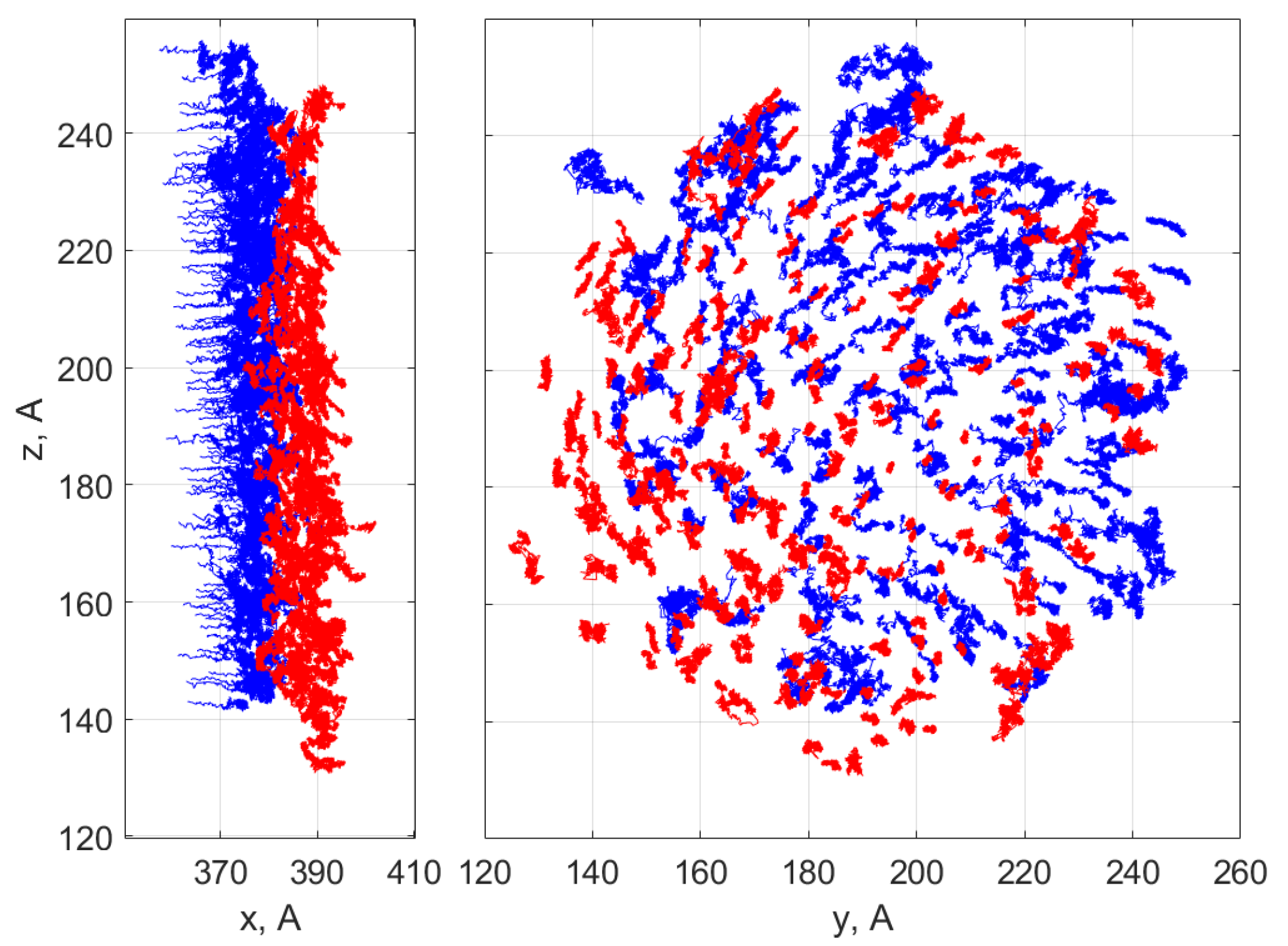
To analyse the diffusion process underlying the sintering, the trajectories of atoms that arrive in the boundary layer are tracked backwards in time, using the “prehistory approach” [
47]. The corresponding trajectories of the Ti atoms forming the grain boundary structure are shown in
Figure 3. The drift and diffusion coefficients of the atoms were calculated using a standard approach [
48]. The trajectories of
3460 and
4450 Ti atoms were followed within the left and right particles, respectively. A small subset of these trajectories is shown in
Figure 3. Each trajectory
has length
2300 and sampling times
with time step
0.4 ps.
Following this approach [
48] the drift velocities (
) are found as
where
. Similarly, the diffusion matrix
where
is
Note that Equations (
1) and (
2) correspond to the values of drift and diffusion averaged in time over the atom trajectories that form the grain boundary at 1 ns and therefore should be considered as being order of magnitude estimates. It appears that MD simulations substantially overestimate the drift coefficient as
70 mm/s, while providing reasonable values for the diffusion coefficient with values ranging from
m
/s to ≈
m
/s. The overestimation of the drift coefficient is probably related to the unaccounted rotation of the system around the axis of symmetry that connects the centres of the particles, which can be noticed in
Figure 3 (right).
Importantly, MD simulations provide estimation for another key quantity of the system—the effective grain boundary width
—that will be used below to estimate sintering stress and sintering time in the phase-field model. It can be seen from the
Figure 2 that
depends on time and quickly becomes ≳10 Åafter approximately 0.5 ns of simulations of the particles with diameter
D = 24 nm. It can also be seen that the width of the grain boundary is closely related to the geometry of the neck and can be expected to scale nearly linearly with the radius of the particle. It may be expected, therefore, that
is of the order of
for particles of micron size.
The latter inference may clarify the situation in phase-field modelling of sintering. In the latter theory (see below) it is often assumed that the actual value of the is ≈ Å. Because this value is unsuitable for phase-field simulations, it is, therefore, re-scaled to on the assumption that such re-scaling does not change the dynamics of the model. However, this assumption is incorrect and is also unnecessary: it has been shown above that is a natural value of grain boundary width for the particles whose diameter is ∼ .
The main results of this section that will be used for the estimation of the sintering stress and microstructure evolution include estimations of the important sintering parameters. It was shown that the grain boundary width
is of the order of ∼
for particles of diameter ∼30
, while the value of the surface diffusion coefficient
was estimated to be in the range ≈
m
/s to
m
/s, while drift coefficients were significantly overestimated due to unaccounted rotation of the samples around the axis of symmetry. Molecular dynamics can evidently provide important insights into the mechanism of diffusion and can yield estimated values of the diffusion coefficient and grain boundary width. These parameters are also important for other theories including those of Coble [
5] and Wakai [
49], and for the master sintering curve method [
50]. At present MD has a number of weaknesses, mainly related to the limited computing power [
19] available. The size of the particles is limited to 30 nm in diameter and the time of simulations is of the order of 100 ns. However, it is expected that the MD will be able to handle larger numbers and diameters of particles in the near future due to ongoing hardware and algorithms development.
3. Microstructure Evolution
One of the most important issues in modelling sintering processes relates to the formation and growth of grains [
7]. Sintering can be divided into four stages [
7]: (i) contact formation, when weak atomic forces hold particles together prior to sintering; (ii) neck growth, when each contact enlarges without interaction with neighbouring contacts; (iii) pore formation, where neighbouring necks grow and interact to generate a network of pores; (iv) pore closure, where discrete pores are formed.
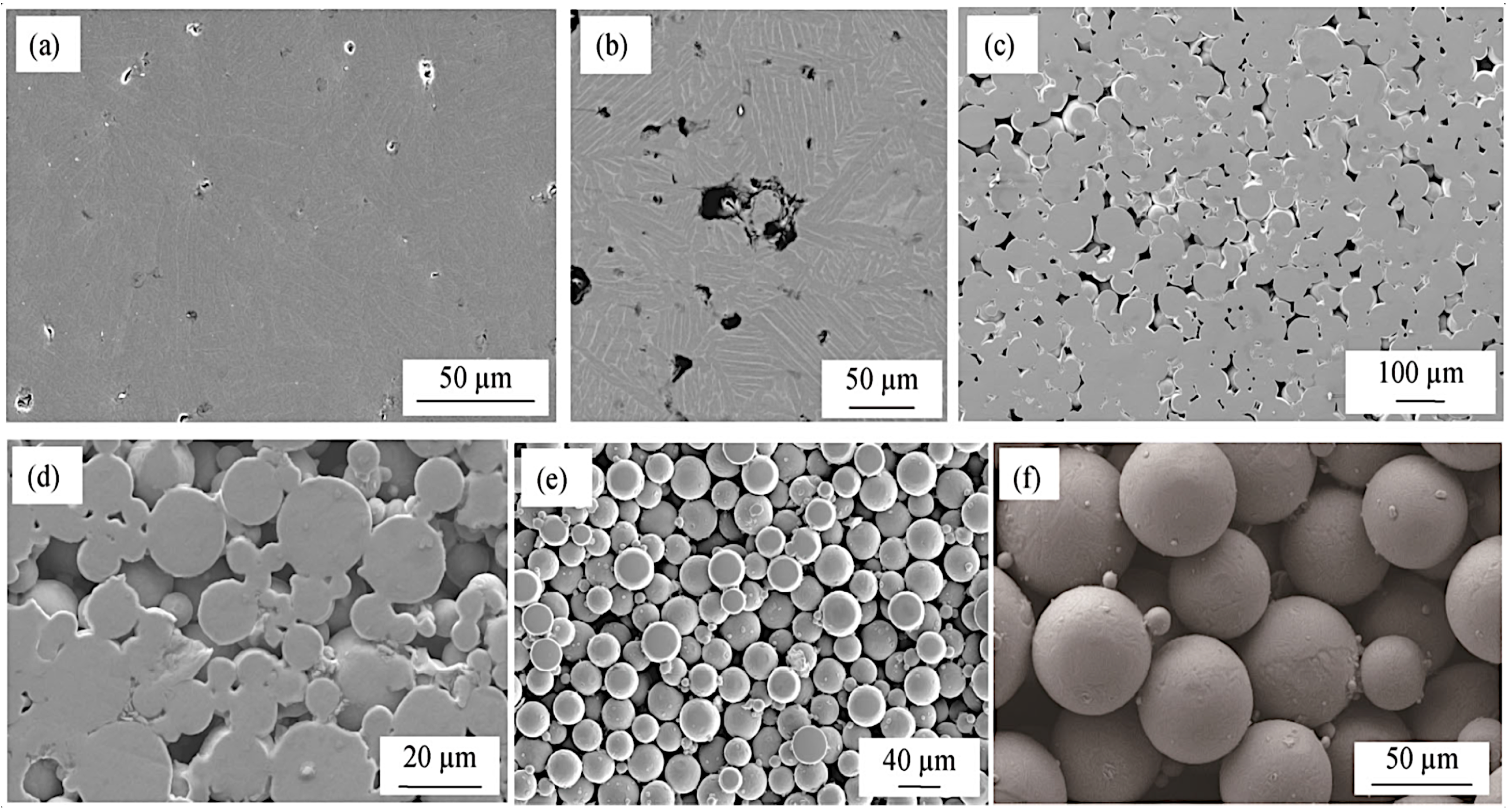
Scanning electron microscopy (SEM) provides deep insight into the evolution of the microstructure during these sintering stages, see, e.g., the SEM images of Ti6Al4V samples prepressed at 500 MPa and sintered at low temperatures shown in
Figure 4. Results are shown for three different particle sizes (0–20, 20–45, and 45–75
m) and two different sintering temperatures (900
C and 1260
C). The heating rate in these experiments was 25
C/min and the holding time was 1 h. A number of important features can be seen in the figure.
First, note the strong dependence of the sintering results on the temperature. In particular, samples with particle sizes 0–20 m sintered at 1260 C are in the final sintering stage (iv), while samples sintered at 900 C are still in transition from stage (ii) to stage (iii). Samples with particle sizes 45–75 m sintered at 900 C are at the stage of green samples in transition to stage (i), while the samples sintered at 1260 C are in transition from stage (iii) to stage (iv). These results are to be expected because sintering is governed by diffusion processes that depend exponentially on temperature.
Secondly, the results indicate that the sintering rate depends strongly on particle size. This observation can at least partially explain the overestimation of the sintering rate observed for nanoparticles in molecular dynamics simulations discussed in
Section 2.
The set of states shown in
Figure 4a–f also provides a good illustration of the different sintering stages, starting from the initial state (f) of nearly intact spherical particles, following to the initial necking state (e) where nearly intact spherical particles are weakly linked by necking, then to the final necking state (d) when the particles begin the transformation into the grains, followed by the grain growth (c) and pore shrinkage (b) to the final stage (a). This evolution is to a large extent generic, as discussed, e.g., in [
7].
It is exactly this set of nonlinear transformations of the microstructure which is difficult to model. The phase-field method [
14,
15,
16,
51] has emerged as a powerful and flexible quantitative solution to this problem, including modelling the evolution of microstructure and the physical properties of metal powder on the mesoscale. Within this approach the evolution of the microstructure is defined in terms of the free energy
F of the system defined as
where the terms correspond respectively to the bulk free energy
, interfacial energy
, elastic strain energy
, energy terms due to thermal field
, and external field
.
Within this approach, a set of phase-field variables is used that are continuous functions of time and spatial coordinates. A distinction is made between conserved and non-conserved variables. Conserved variables are typically related to the local composition. Non-conserved variables usually contain information on the local (crystal) structure and orientation. Order parameters and phase-fields are both non-conserved variables that are used to distinguish coexisting phases with different structures. The order parameters
refer to crystal symmetry relationships between coexisting phases [
52]. Phase fields are phenomenological variables used to indicate which phase is present at a particular position in the system. In a system with
N components, each having the number of moles
(
), the following conservative variables can be used [
51]: mole fraction
and molar concentration
of
i-th component
where
is the total number of moles in the system,
the molar volume and
V the total volume of the system.
3.1. Model Equations
In the phase field approach the microstructure evolution for variables
and
is modeled by a set of coupled Cahn–Hillard (CH) and Allen–Cahn (AC) phase-field equations
These equations are derived from the free energy functional
F of isothermal sintering of metal particles [
15,
53]
with the internal phase-field free energy given by
In Equation (
3),
A and
B are constant parameters with units of
, and
and
are coefficients of the surface and grain boundary energy gradients with units of
and
are the surface and the grain boundary energies,
is the grain boundary width. Note that the choice of the grain boundary width in the phase-field method is a subject of continuing discussion. E.g., in the work [
16,
54] the
is taken of the order of 1
that corresponds to the boundary layer of atomically clean interface between metallic grains. On the other hand
is often assumed to be of the order of the mesh size (i.e., ∼1
) [
51,
55] or to have intermediate value, e.g., 60
[
25] The results of the MD simulations discussed in the previous section will be used to estimate the effective width of the boundary layer
, which is shown to be of the order of 1
. This value was used in the phase-field calculations below.
M and
L are CH and AC mobilities with units
and
respectively.
M is calculated from the diffusion coefficients as [
15]
where
and
,
,
, and
are respectively the coefficients for atomic mobility in solid bulk, vapour, along the surface, and along the grain boundary given by
with
where
and
are the corresponding diffusion coefficients and activation energies,
is the Boltzmann constant and
T is the temperature.
A nondimensional form of the AC and CH equations is [
56]
In the simulations the size of the 2D region is of the order 100 × 100 pixels corresponding to an area of ∼100 × 100
2,
, the value of
is taken as ∼
, which was shown in the previous part
∼
to be a natural length scale of the problem. The mobilities are defined as
Examples of parameter values for this problem are given by e.g., Biswas et al. [
15] for tungsten, by Zhang [
53] for Ti and Ni, by Wang [
57] for TiAlV alloy, and by Ahmed [
54] for CeO
. In the present work the following model parameters were used:
J/m
,
J/m
,
J/m
and
J/m
,
J/m, and
J/m,
m
/(J·s) and intrinsic interface mobility
m
/(J·s), cf. [
57]. The diffusion mobility
M given by Equation (
7) usually relies on diffusion coefficients that are found experimentally. Values of the diffusion coefficients were also estimated by MD simulations, see
Section 2. The molar volume of Ti was taken to be
cm
/mol (or atomic volume
m
) and the relationship between
L and the grain boundary mobility
to be
.
3.2. Mechanical Loading
To include the effects of external loading and gravity, the phase-field model needs to be coupled with elasticity. Such a coupling with the phase-field equations is usually introduced within the theory of structural transformations in solids [
58]. The governing equation within the domain
and boundary
can be stated as follows:
where
is the Cauchy stress tensor,
is an additional source of stress (such as pore pressure),
is the displacement vector,
is the body force per unit volume including gravity,
is the unit normal to the boundary,
is the prescribed displacement on the boundary, and
is the prescribed traction on the boundary. The gradient of stress has units
.
Within the theory [
58] the elastic energy has to be added to the total free energy (
4). For the elastic energy calculation, the elastic strain (
) is computed from the displacements, and corresponding stresses (
) from Hooke’s law; for further details see [
16]. The resultant elastic free energy is of the form
where the material stress response is described by the constitutive model, in which the stress is determined as a function of the strain
, e.g.,
, and
is a stress free strain. For example, the elasticity is assumed to be linear for small strains, i.e.,
where
is the elasticity tensor. The model Equations (
3)–(
10) are solved in MOOSE Multiphysics [
14,
16].
3.3. Results
Numerical simulations of the particle sintering model given by Equations (
3)–(
10) are performed using phase-field and mechanics modules in the MOOSE Multiphysics [
32] environment. The simulations were performed using 2D and 3D phase-field models of sintering.
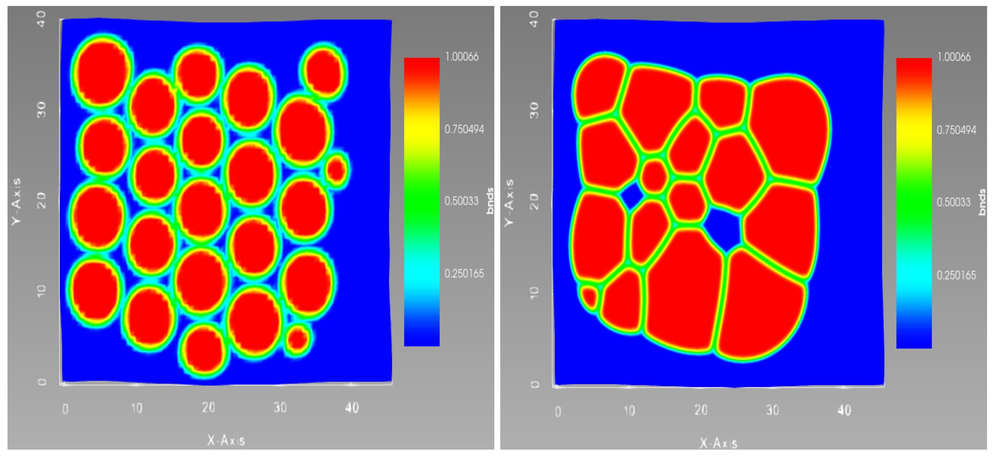
Results of the 2D Simulations are shown for 23 particles in
Figure 5 with zero gravity and periodic boundary conditions.
It can be seen that the phase-field model reproduces the transformation from particulate to dense granular structure of the samples shown in
Figure 4c–f. This model also provides insight into the faults developed during such transformation, as shown in
Figure 5 (right), which is consistent with the experimental observations [
56]. The formation of the defects both between the particles inside the filament and between filaments can be reproduced by the model. In particular, open pores shown in
Figure 5 (right) correspond to the open pores that can be seen in the
Figure 4c. A set of interconnected open pores corresponds to the lack of fusion defects observed experimentally in [
28]. The formation of such defects will depend strongly on the initial distribution of the particles, as will be further discussed in
Section 4.
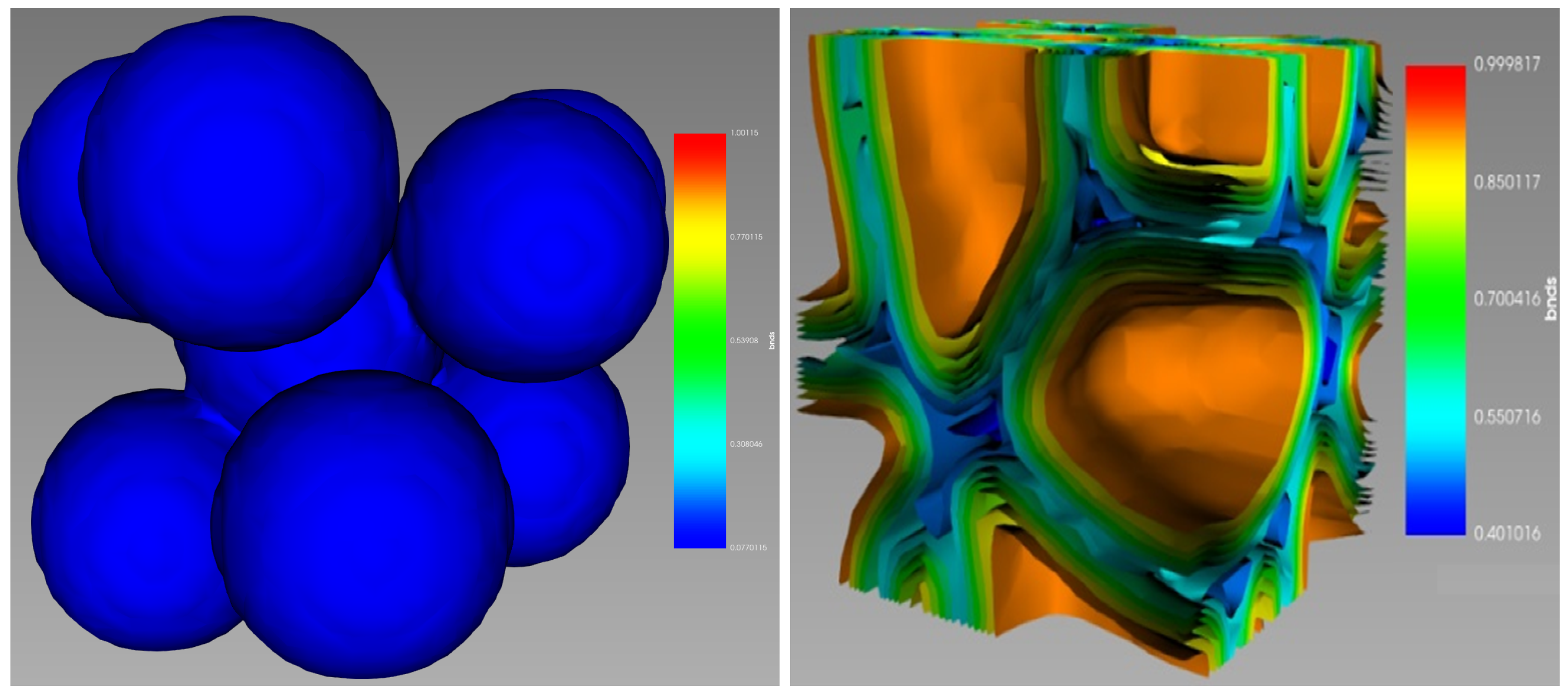
The 3D phase-field models can be further used to estimate the sintering stress and time scales. Results of the phase-field simulation of 3D sintering of metal particles are shown in
Figure 6. The simulation domain was
= 27 × 21 × 12
m
and the mesh size was 40 × 40 × 30. The dimensionless parameters used in the simulations were
A = 16.0,
B = 1.0,
L = 1.0,
= 1.0, and
= 0.5, see also [
15]. The preconditioned Jacobian Free Newton Krylov solution method was used with an initial time step of 0.001 and a growing factor of 1.1. Note that, at present, the number of particles in simulations is limited to just a few. To speed up the simulations, the mesh adaptation was excluded, accordingly, the results can be considered only as order of magnitude estimates. Yet, the simulations remain time-consuming, cf. [
59]. An example simulations for 9 particles during 20 dimensionless time units took about 36 h, using 32 threads of the Threadripper 2990WX.
The evolution of the free energy and the internal boundary of this system are shown in
Figure 7. It can be seen from the figure that initially round particles are transformed into grains with a number of grain boundaries similar to those observed experimentally in [
60]. These results will now be used in the next section for estimation of the sintering stress.
Sintering Stress
To estimate the sintering stress from the results of the PFM simulations, note that the corresponding pressure scale can be approximated by the Laplace pressure in the form [
61,
62]
, where
is the mean particle radius and
is the surface tension. For the
J/m
and
∼ 10
m it can be shown that
Pa. The sintering stress is in general defined [
21,
62] as
where
F is the free energy and
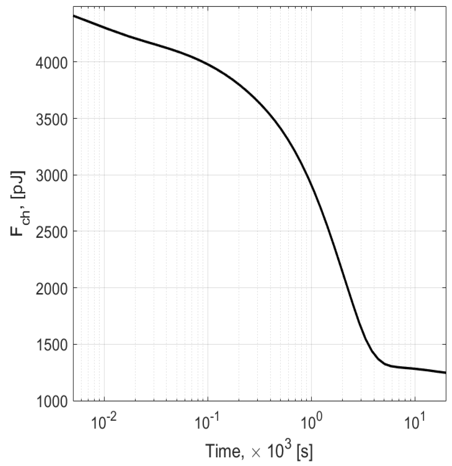
V is the volume occupied by the particles. The time evolution of the free energy is shown in
Figure 7. Its shape correlates strongly with the shape of the shrinkage dependence on time shown in Figure 2 of Ref. [
6], i.e., a nearly flat initial region followed by a sharp decay of the free energy
F, corresponding to rapid shrinkage of [
6]. Finally, a slow decay of the
F is observed for large times, which again is strongly correlated with the slow shrinkage region observed in [
6] for large times.
Such a strong correlation originates in the mechanism of sintering, which follows the four stages [
7] listed at the beginning of
Section 3 and illustrated in
Figure 4. According to this mechanism, the initial rearrangement of particles at low densities leads to contact formation and necking, followed by independent neck growth. Necking and neck growth correspond to the sharp shrinkage and decay of the free energy.
Independent neck growth is followed by pore formation, and slow diffusion of pores to the sample surface. The pores occupy a relatively small volume of the sample. Their diffusion is relatively slow and corresponds to the slow regions observed in shrinkage and decay of the free energy discussed above. To estimate the sintering stress, note that the change of the free energy
in the
Figure 7 is given in pJ, while the change of the particle’s volume
corresponds to the change of relative density of the particles from ∼0.3 to ∼0.96 of the simulation domain volume
. This yields the following value for the sintering stress in (
11):
Pa.
Another way to estimate the sintering stress is to notice that the initial free energy can be written in the form
where
is the number of particles, and
is the surface area of the
i-th particle. For a crude estimation, the final free energy can be taken as zero, while analysis of the intermediate state can be done by assuming that all the particles have the same volume but their shape is changed to the space-filling polyhedra, cf.
Figure 4c,d. Consider, for example, a truncated octahedron, for which volume
and surface area
are known as a function of the edge length
aThis allows one to calculate
for the metal particles and to estimate intermediate surface energy by noticing that all the particles are in full contact with each other
where the factor
is included to avoid double counting of the octahedron’s surfaces.
The corresponding change in the volume of the system of particles can be found as above, which gives the following estimate for the sintering stress Pa.
To conclude this section it is pointed out that the phase-field model provides deep insight into the microstructure evolution of the system during sintering and can reproduce the transformation from particulate to dense granular structure of the samples, as observed in the experiments. It can also be used to estimate qualitatively the fault development during such transformations, which can then be compared with the experimental observations. 3D phase-field models can be used to estimate sintering stress and other parameters required for modelling the sintering of full-size parts. This model was applied to simulate the microstructure evolution in the cross-section of one filament. In 2D this approach allowed modelling of the sintering of a few tens of “particles” with diameters of the order of a few microns, on the time scale of hours. In 3D the number of particles had to be reduced to ten. The values of the sintering stress were estimated to be of the order 1 MPa. These results agree with experimental observations and can further be used for finite element modelling of the whole part.
Next, an approach is considered that can be used for modelling initial shrinkage in submodels that include tens of thousands of particles. This approach allows for particle resolution and provides estimates of the mass distribution in the sample that takes account of the filament layout and the initial rearrangement of the particles.
4. Discrete Particle Model
This section considers modelling of initial sintering stage within a framework of the discrete element method (DEM) [
17,
18,
19,
20] based on a new generalised viscoelastic model of sintering proposed in [
17]. Within this method the translational and rotational dynamics of the particles are resolved by integrating [
63] the Newton’s equations of motion. For the
i-th particle,
where
is the element’s centroid displacement in a fixed (inertial) coordinate frame,
the angular velocity,
is the element mass,
is the moment of inertia,
is the resultant moment about the central axes, and
is the resultant force including external forces such as gravity. The important component is the contact force
, which is divided into the normal and tangential sub-components,
and
, respectively
The normal part of the contact force can be further divided into sintering
and viscous resistance
forces: Rojek et al. introduced the following approximation [
19] to the normal component of the contact force
where
is the normal relative velocity,
r is the particle radius,
a is the radius of the interparticle boundary,
is the dihedral angle, and
is the surface energy. The effective diffusion is dominated by the grain boundary diffusion mechanism and can be approximated as
where
is the grain boundary diffusion coefficient,
is the width of the grain boundary,
is the atomic volume,
is the Boltzmann constant, and
T is the temperature.
The constitutive relations take the form [
19]
where
is the Cauchy stress tensor,
C is the elastic stiffness tensor,
is the sintering driving stress, and the strain rate
is decomposed into the elastic, thermal and viscous parts,
,
and
respectively.
The DEM approach was used to model rearrangements of particles at the initial stage of sintering in realistic geometries and filament layouts. A discussion of some results of simulations is presented in the next section. The discrete element model of particle sintering was developed in KRATOS Multiphysics [
33,
34]. The contact forces [
18] between two particles were modelled using the Hertz model with JKR cohesion [
64] as a sum of elastic and viscous components. The elastic part assumes a linear force–displacement relationship
where
is the particle’s penetration and
k is the contact stiffness. The viscous component is assumed to be a linear function of the normal relative velocity
and the viscosity coefficient
c can be taken as a fraction
of the critical damping
for the system considered
where
and
are the masses of two particles and
k is an effective spring stiffness.
This model was used to analyse shrinkage as a function of the filament layout and gravity. The effect of these factors on nonlinear shrinkage was of particular interest, as was changes in the microstructure of the samples at the initial stage of sintering.
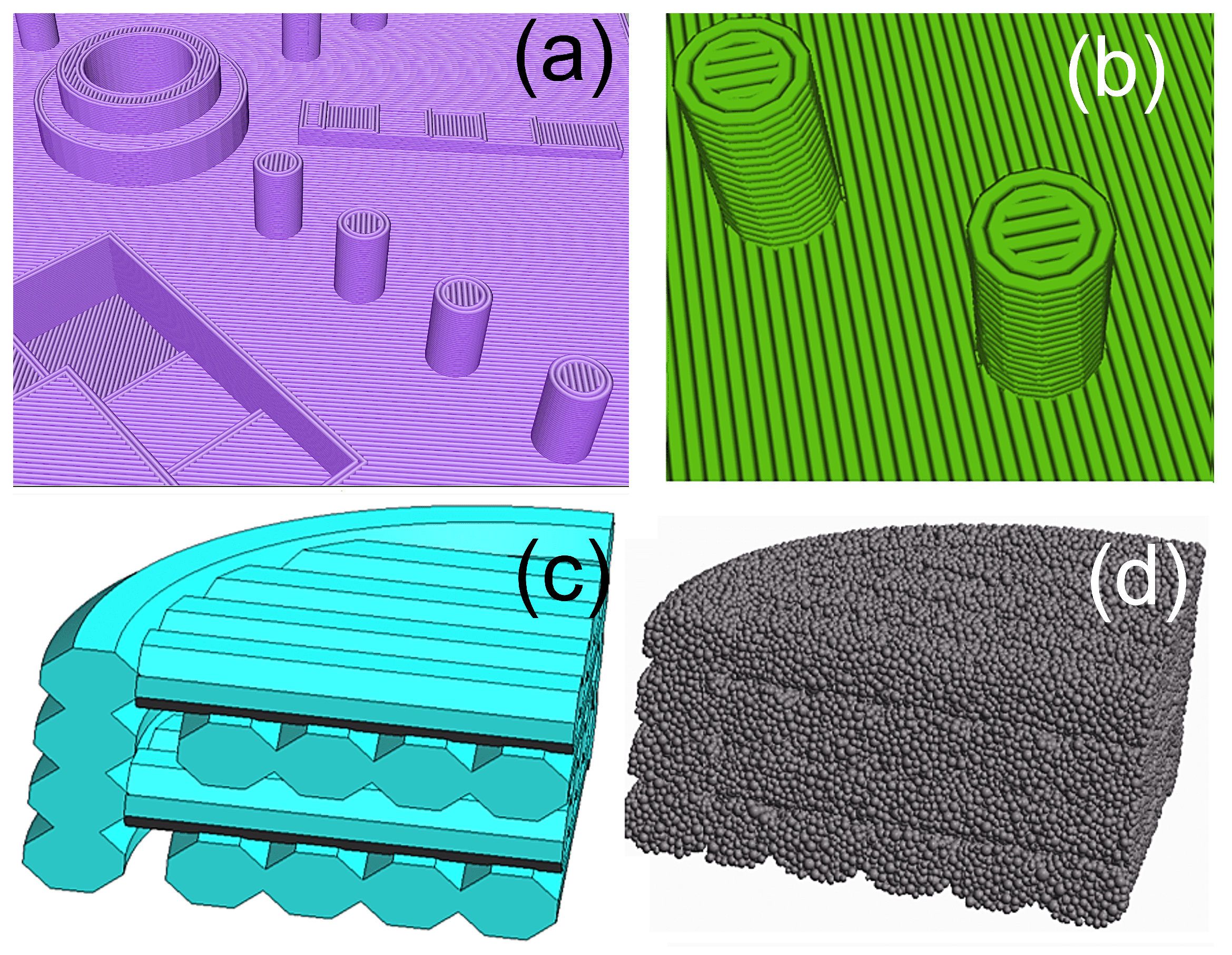
The effect of the filament layout on nonlinear shrinkage was simulated in a submodel of the NIST test artefact (see
Figure 8) using the DEM Application in KRATOS [
33,
34]. The model of the artefact was sliced using Repetier-HOST v.2.1.6 slicer, see
Figure 8a. Next, a small subsystem, the cylinder shown in
Figure 8b, was selected for further analysis. Finally, sub-models of the cylinder with different filament layouts were constructed.
The sub-models were built in SALOME v9.3 [
65] for two different filament layouts: (i) crossed layers and (ii) all layers are laid in the same direction. The STL files of sub-models were imported into KRATOS Multiphysics. Simulations were conducted using the DEM application. The resultant geometry for cross-layers and the final mesh for unidirectional layers are shown in
Figure 8c,d, respectively. The material parameters chosen for the simulations are shown in
Table 2.
The resultant shrinkages for unidirectional and cross layouts are compared in
Table 3. The Young’s modulus and cohesion used in these simulations were
Pa and
Pa respectively (other parameters are shown in
Table 2). The default porosity was 56%. The total number of spherical articles in these simulations was ∼150,000.
For example, the table shows the following shrinkage for the unidirectional layout (left half) in x-, y-, and z-directions: , and . These results indicate that shrinkage in the horizontal plane is nearly the same in x- and y-directions while shrinkage in the z-direction is slightly larger. Similar results are obtained for crossed layout of the filaments. The corresponding shrinkage is: , and indicating that, for the crossed layout, shrinkage in all the directions is slightly smaller than for the unidirectional layout.
Repeating the simulations for this set of model parameters [
56] revealed a weak dependence of the shrinkage on the filament layout. In most cases, the initial shrinkage is smaller in the vertical and horizontal directions for cross-layout as compared to the unidirectional layout. This trend is more pronounced for an increased initial porosity. However, the dependence is weak and depends on model parameters such as Young’s modulus, cohesion energy, and gravity. The latter strongly affects nonlinear shrinkage as will be discussed next.
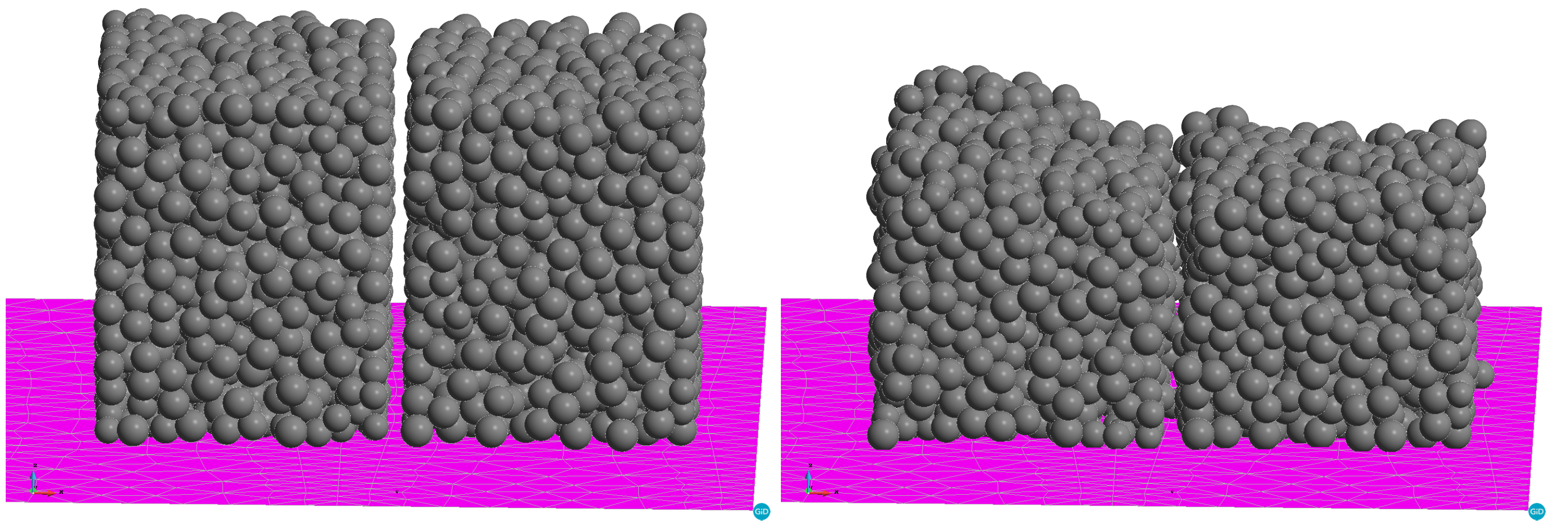
The effect of gravity was analysed by simulating two rectangular cuboids built of spherical metal particles. The latter are allowed to evolve under the action of gravity and interactive forces between the particles, on the ground, and in microgravity. The results of the simulations under normal gravity conditions are shown in
Figure 9. These results are well reproduced. The cuboid dimensions in this sample are
mm. The volumes of one cuboid and the spheres are
mm
and
mm
respectively. Accordingly the initial porosity is ∼0.57 (fractional density ∼0.43). It can clearly be seen from the figure that the initial shrinkage is strongly nonlinear. Shrinkage in the
z-direction is ∼0.22 while the sample practically does not shrink in the horizontal plane. The final porosity is ∼0.42 (fractional density ∼0.58), which corresponds approximately to the estimate of particle density in the filament in
Figure 8. The lower the initial density, the larger the observed shrinkage in the
z-direction. Note that the initial gap between the two filaments ∼
remains nearly intact to the end of the simulation. These results confirm the assumption that gravity on the ground can contribute significantly to the nonlinearity during the debinding and earlier sintering stages when the initial fractional density of the samples is less than ∼55%.
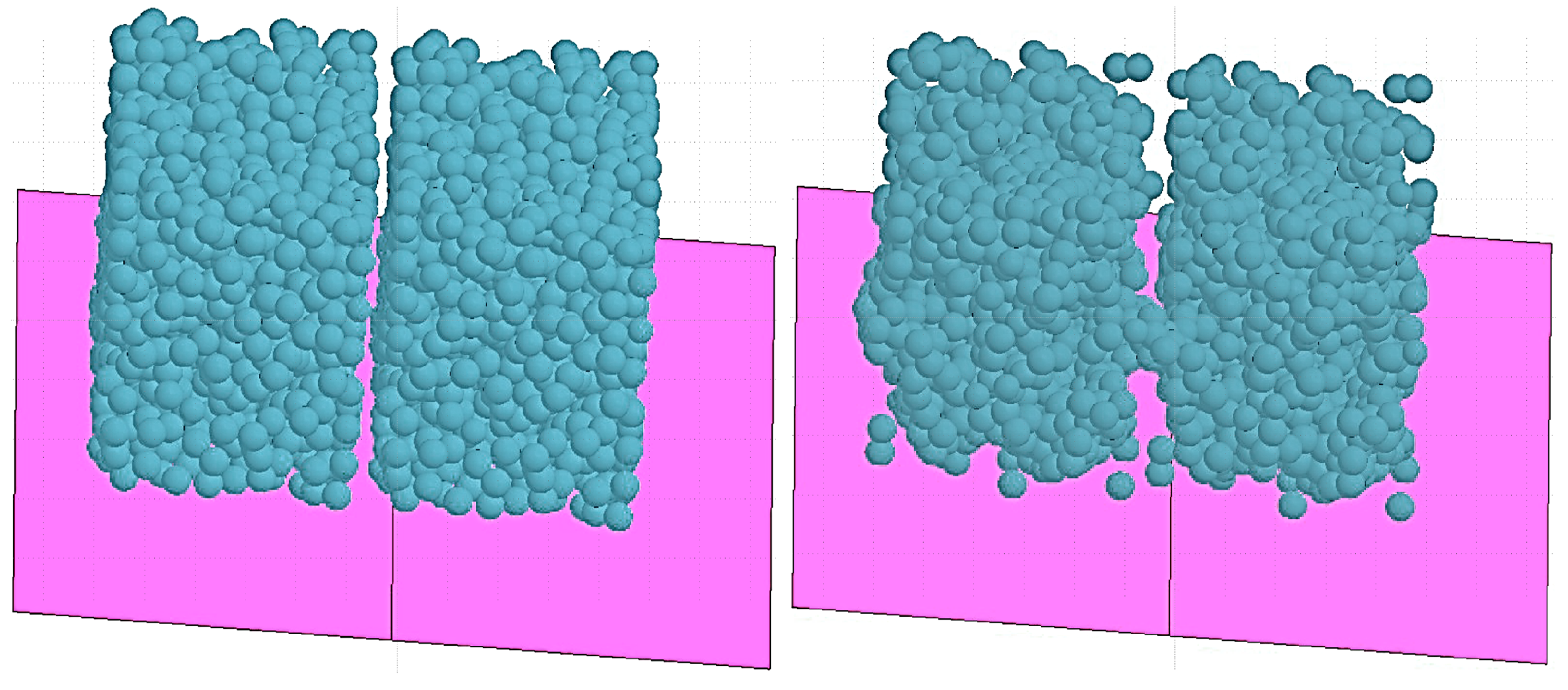
To analyse the effect of microgravity, simulations of the same samples were performed under zero gravity conditions. The comparison of the samples’ structure before and after shrinkage in microgravity is shown in
Figure 10. The final fractional density of the samples after rearrangement of the particles under microgravity was found to be ∼0.48. One can see that under zero-G conditions there is no significant shrinkage in any direction as shown in
Figure 10. Instead, agglomeration of the particles and the formation of large pores are evident in the figure. Therefore, sintering under zero-G conditions may result in a higher probability of regions where there is a lack of fusion [
27,
28] as will be discussed in more detail in
Section 5.
Note that the discrete element method considered in this section provides important insight into the initial shrinkage of the filaments, but has some limitations both in accuracy and in the range of applications. Therefore, the DEM approach was mainly used to estimate the initial rearrangement of the particles, gravity-induced nonlinear shrinkage, and the spatial distribution of mass in the samples prepared in zero gravity. The model developed in KRATOS Multiphysics [
33,
34] allowed simulation of the translational and rotational motion of hundreds of thousands of interacting particles using the discrete element method. It was revealed that gravity is a major source of the strong non-linear shrinkage observed in experiments on the ground, while in zero-G, the shrinkage is only weakly depends on the filament layout and the spatial direction. It was also demonstrated that sintering in microgravity may result in the agglomeration of particles and increased risk of fault formation, including lack of fusion. These data were further used to develop a simple model of shrinkage and as input parameters in finite element modelling of sintering of the whole part.
6. Macroscopic Modelling of Sintering
Modelling shrinkage for the full-size parts was performed using the continuous finite-element method in commercial software COMSOL Multiphysics
[
35]. In the simulations, the model parameters were kept close to those used experimentally in sintering Ti-6Al-4V alloy [
56], which are also consistent with the simulations of the previous sections. Powders of this metal can be combined e.g., with some polymer mixtures to form feedstock for fused deposition modelling. Importantly, the softening temperature of compatible binder materials must be substantially lower than the melting temperature of the metal powder enabling filament printing through an extrusion method with subsequent debinding and sintering stages as described in the introduction, see also [
4,
56].
The simulations used typical structural parameters for the modelled material, noting that the green part was produced by printing filaments. Two different powders were considered, both coarse and fine [
56,
80]. It was further assumed that thermal debinding was achieved using a heating rate of 1–2
/
with 3 h holds at three different temperatures between 200
and 500
in low pressure to produce the brown part. Subsequently, the brown part underwent the 3 h sintering process at temperature above 1200
in a low pressure environment.
To simplify modelling it is assumed that thermal debinding of the green part was performed without shrinkage and collapse of the structure. The shrinkage of the sintered part was considered at the sintering stage. In this case a large fraction, e.g., 40%, of the sample volume after debinding is an empty space. Some residual binder (a backbone) may still be present until sintering starts to keep the brown part from disintegrating in zero gravity. Thus the initial stage may involve removal of the residual binder, necking and strong adhesion among the adjacent particles, causing the shrinkage of the part by ∼10%: see the previous section. Subsequent sintering takes place in a vacuum or in an inert gas [
81].
After thermal debinding, only a small amount of residual backbone binder is left, mostly located in inter-particle pockets. In this case two mechanisms of sintering could be considered. The first one is due to sintering stress induced by the residual binder, and the second is due to shrinkage of the solid continuum. The first mechanism is due to viscoelasticity and creep behaviour. These phenomenological mechanisms will now be used to provide qualitative results for sintering and shrinkage.
6.1. Equations for Modelling Metal-Fused Filament Fabrication Process
The rheological theory of sintering developed by Skorohod [
82] is based upon the phenomenological concept of the generalised-viscous flow of porous bodies. These ideas were further extended by Olevsky [
21,
22] by including, in particular, relationships between rheological parameters (such as bulk, shear viscosity and the effective sintering stress) and deformation of a viscous porous body under sintering.
Two stages of shrinkage are considered: debinding of the backbone polymer at a temperature close to sintering and the sintering itself. In addition, some properties of the sample obtained by metal fused filament fabrication (mf3) will be modelled. Dimensional change during the “mf3” process, shrinkage or swelling, can be predicted from continuum mechanics. During the debinding stage, the binder is burned out and removed from the furnace chamber, while the pores are filled by air or inert gas. The corresponding solid system transformation is modelled by solving systems of coupled continuous equations for solid state media, including for diffusion, and heat transfer. In addition, an account is taken of binder diffusion activated by temperature and the medium changes during debinding.
The corresponding dimensional changes are the result of changes in viscosity and the sintering stress. Because experimental parameters for these processes are not known, phenomenological parameters introduced on the basis of the underlining physics are used instead.
In the simulations, the Ti-6Al-4V metal powder bound by the polymer subsystem is modelled as a continuous medium. The goal is to determine the shrinkage after the two stages of debinding and sintering. It is assumed that in the final stage of sintering the density of voids corresponds to the experimentally observed value of ≈5%. It is further assumed that the main shrinkage happens during the sintering of the metal part. In the next subsection, the modelling results are considered in more detail.
6.2. Constitutive Relations for Olevsky Model
The material response to loading and deformation is modelled using elastic
and viscous
components, cf.
Section 4,
where
is stress,
is strain,
E is a Young’s modulus, and
is a viscosity. There are two different viscoelastic models to consider: (i) the Maxwell model
consisting of a spring term and a dashpot term placed in series where the first part is an elastic law and the second term is a creep; (ii) the Voigt–Kelvin model
representing a solid undergoing reversible, viscoelastic strain. The constitutive Equation (
22) leads to Riedel’s model [
83], while Equation (
23) leads to the generalised Olevsky model [
21,
22]. The strain rate in the phenomenological sintering model consists of the equivalent elastic strain rate
, thermal strain rate
, and creep strain rate
, cf. Equation (
14). It is the last term that is responsible for sintering.
Olevsky’s constitutive model [
21] is given by the equation
where
is the apparent viscosity of the porous body skeleton,
is the effective sintering stress, and
is the Kronecker symbol.
and
are the coefficients of effective shear and bulk moduli, respectively
Here porosity
is defined as the ratio of the pore volume
, to the total volume
. The sintering stress in the case of free sintering (
= 0) is
where
is the mean radius of powder particles,
is the surface tension, and
is a free volume shrinkage.
Equations (
25) and (
26), and the continuity equation for mass conservation
yield
For time-independent coefficients, the solution of this equation is
where
is the initial porosity and
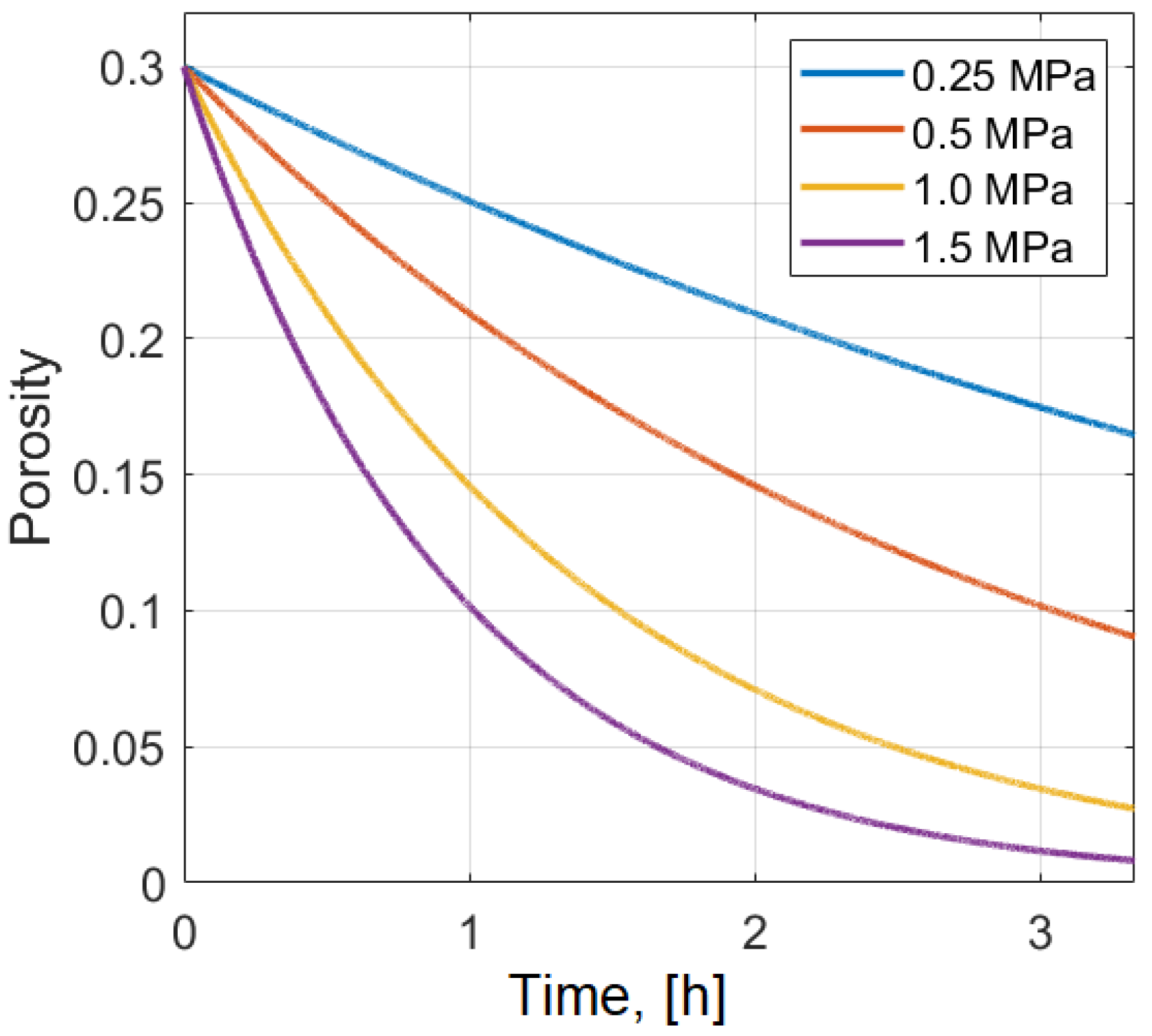
is the characteristic sintering time for continuum models. The effect of the sintering stress on the dynamics of porosity is illustrated in
Figure 14. This dependence is a function of the viscosity and sintering stress. It can be seen from the figure that the higher the sintering stress the lower is the final porosity and the higher is the shrinkage. For the characteristic value
Pa and with a typical sintering time of ∼3 h, the viscosity should be of the order
–
Pa
s. This implies that to reduce the sintering time the sintering temperature needs to be sufficiently close to the melting temperature in order to reduce the viscosity.
6.3. Simulation Results for the Olevsky Model
The commercial software COMSOL
[
35] was used for simulation of the sintering process. In addition to the solid state structural module, the Domain ODEs and DAEs mathematics were used for porosity modelling. The viscoelastic properties were taken into account by using the Kelvin–Voit approach. Some simulation experiments were undertaken to check limiting cases [
56]. First, consider the case of zero gravity and no sintering stress, while keeping low viscosity 10
Pa
s. In this case the initial porosity distribution (
= 0.3) did not change after 3 h of sintering. Similarly, there were no changes in the displacement and stress since no external or internal stresses were applied. In the second numerical experiment gravity was applied. In this case the simulations exhibited small changes in porosity, displacement and stress. These changes depended on the value of the viscosity: the lower the viscosity, the larger were the changes.
For the sintering stress = 0.5 MPa, viscosity Pas, the initial porosity = 0.3, and sintering time ∼3 h the porosity was reduced to 0.09 corresponding to shrinkage of about 7%. The distribution of the porosity in the vertical direction remained homogeneous in the absence of gravity and became slightly inhomogeneous (≤0.1%) in the presence of gravity. The characteristic stress distribution (von-Mises invariant) displayed practically no stress in the structure. When the viscosity is reduced to Pas and the sintering stress is increased to 1.0 MPa, the shrinkage increases to about 13% in the vertical and lateral directions. The von-Mises residual stress remains sufficiently small.
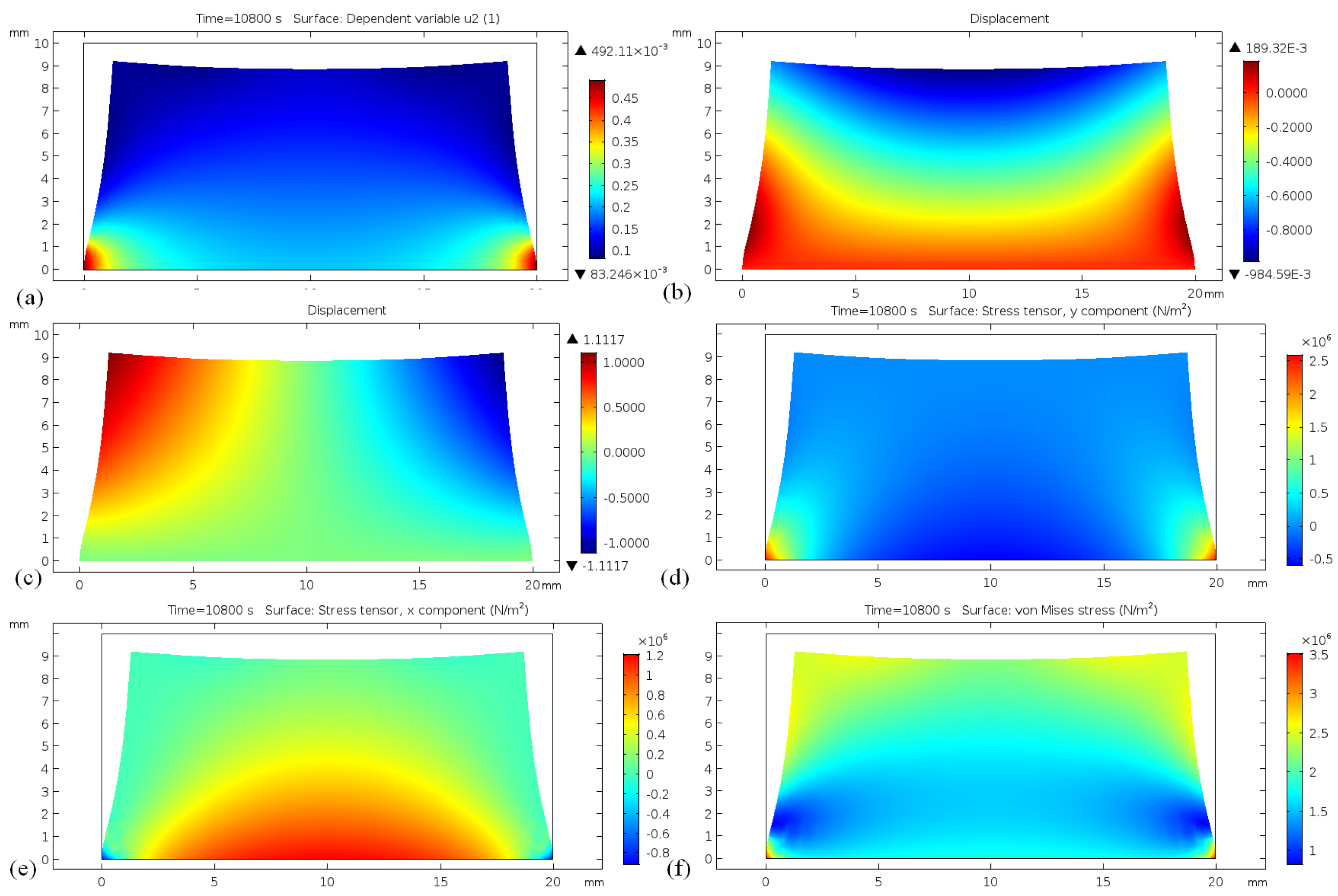
In the next set of simulations the bottom constraint was introduced to keep the dimensions of the bottom pane fixed. Other parameters were
= 0.3,
Pa
s, and
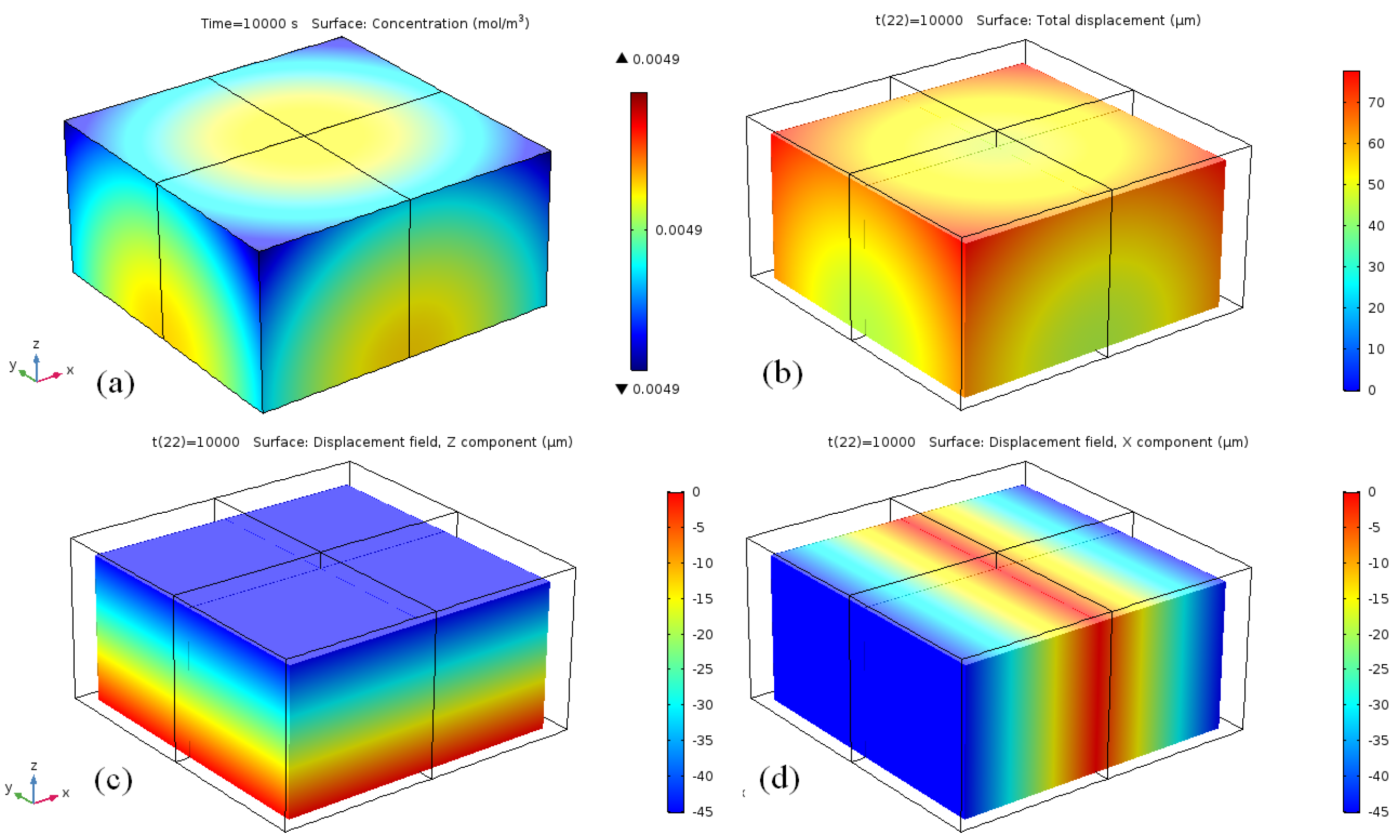
= 1 MPa. The results of the simulations are shown in
Figure 15. It can be seen from the figure that porosity was substantially reduced everywhere except in areas near the fixed corners of the structure. The high porosity at the corners was caused by the nonuniform stress distribution, which was sufficiently high at these locations. The shrinkage of the structure was about 10% in all directions, as shown in
Figure 15b,c. The stress distribution is presented in
Figure 15d–f. It can be seen that inhomogeneous stress
in the
y-direction is at least three orders of magnitude higher in the corners, which might lead to trapping of the porosity
. The analysis is now extended by consideration of shrinkage in the presence of small amounts of backbone polymer.
6.4. Constitutive Model for Backbone Polymer Debinding
To encompass in the model polymer debinding during sintering, it is necessary to take account of thermal diffusion of the binder material. The governing equations for an isotropic, homogeneous elastic solid medium with generalised thermodiffusion are [
84,
85].
where
are components of the displacement vector,
T is the absolute temperature,
C is the concentration of the diffusive material in the elastic body,
and
are Lame’s constants,
is the density, and
and
are material constants given by
where
and
are the coefficients of linear thermal and diffusion expansion respectively.
The constitutive equation for the stress components
is
here
and
are the reference temperature and concentration, and
are the stain components given by:
The diffusion of the polymer binder can be modelled as “moisture" transport governed by the diffusion equation:
where the diffusion coefficient
D is assumed to be of the activation type, cf. Equation (
8)
where
U is the activation energy and
k is the Boltzmann constant. The equations have to be complemented by the equation of thermal conduction
where
is the thermal conductivity coefficient.
The boundary conditions on the exterior faces of the part correspond to a flux of polymer concentration for Equation (
30) and fixed temperature determined by the heating source. For sufficiently slow change of temperature, one can omit the solution of Equation (
31) and assume that the sample follows the heating schedule quasi-statically. This thermally activates the diffusion of the binder at different stages and makes it possible to predict shrinkage.
Within the above formalism, shrinkage can be taken into account by introducing the strain concentration relation
where
is the hygroscopic shrinkage (swelling) coefficient and
M is the molar mass of degraded products of the residual backbone polymer.
To simplify the simulations it is assumed that shrinkage takes place during the debinding of the residual polymer. In this case, the formalism can be applied based on the solution of Equations (
27)–(
31). The parameters of the simulations were chosen as:
m
/kg; initial concentration 10
mol/m
; diffusion coefficient
m
/s; brown part density 3000 kg/m
; Young modulus 10 GPa; Poisson ratio 0.4, for which the part undergoes volumetric shrinkage, consistent with experimental observations ranging from about 12% to 18% (cf. [
11]) for final density ranging from 95% to 99.5% of the theoretical density. To estimate
M in Equation (
32), note that the molecular mass of the degraded polymer is determined by the polymer atoms.
The results of shrinkage simulations for this model are presented in
Figure 16. It can be seen from the figure that, during sintering, the backbone polymer concentration changes by several orders of magnitude and experiences about 10% shrinkage. Similar simulations for a fixed boundary condition at the bottom demonstrate large residual stress leading to higher shrinkage in the vertical direction.
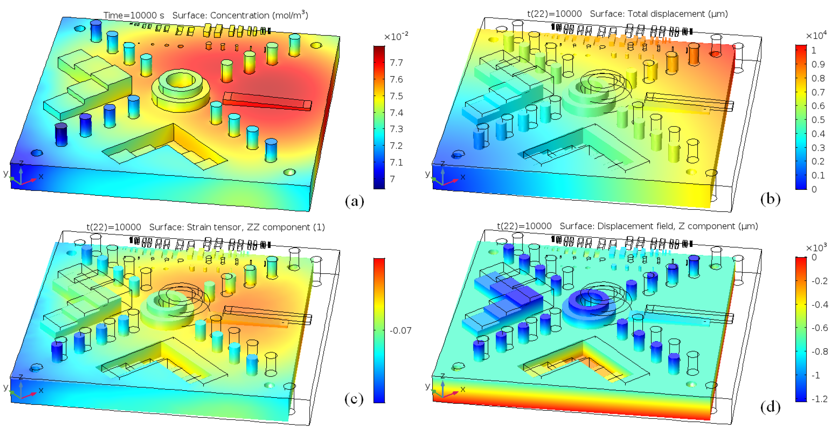
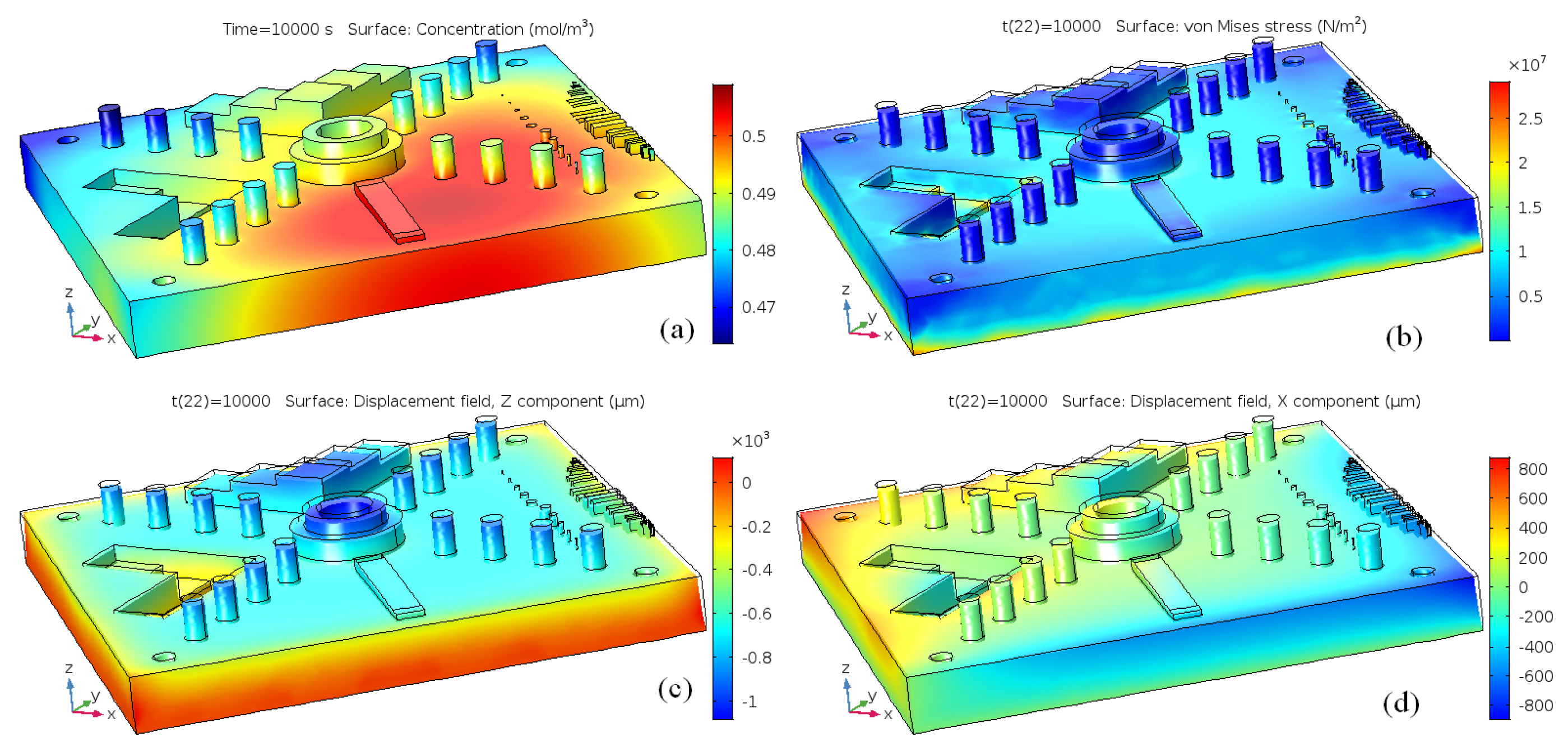
This modelling approach is now applied to the analysis of shrinkage in the whole part, i.e., the entire NIST artefact; see also the CAD shown in
Figure 8a. The results of this modelling are presented in
Figure 17 and
Figure 18. It can be seen from
Figure 17 that all the features of the CAD are reproducible and that the shrinkage is isotropic for the roller boundary conditions. The situation becomes more complex if the boundary condition is fixed at the bottom plane, see
Figure 18. The final part is now deformed in the vertical direction and experiences inhomogeneous deformation in the
X-
Y plane. This means that, for the final part to have the correct dimensions, one has to introduce complex anisotropic compensation to the scales of the green part.
6.5. Nonlinear Shrinkage in Continuous Model
Analysis of anisotropic shrinkage within the continuous model above was performed using two formalisms—the Olevsky model and the debinding model based on thermal diffusion. Both models demonstrate shrinkage of the initial structure. In the absence of constraints at the bottom plane, they both exhibit nearly uniform shrinkage. Anisotropic shrinkage was observed for spatial variation of the model parameters. For example, in the model based on thermal diffusion, the shrinkage rate of the brown part depends on the swelling coefficient, which is a phenomenological parameter and should be determined by experiment for each composition. In the Olevsky model there are two major parameters (viscosity and sintering stress) and the nonlinear shrinkage can arise as a result of spatial variation in either of these parameters. The latter variation can be determined using microscopic simulation discussed in
Section 3 and
Section 4 or measured in an experiment.
For the low initial porosity (
0.35) considered in the simulations, the shrinkage is isotropic and independent of the initial porosity distribution unless an anisotropic sintering stress or swelling coefficient is prescribed. This result is expected because, at such a low porosity, the metal powder behaves as porous metal with uniform high viscosity and high sintering stress; see also discussion in
Section 5.
On the other hand, for high initial porosity (
0.4) the powder behaves as a suspension of metal particles [
71] that displays a very sharp dependence of sintering stress and viscosity on the porosity; see
Section 5. In this case the presence of gravity may lead to significant nonlinear shrinkage similar to that observed in discrete element modelling; see
Section 4. To incorporate the dependence of the viscosity on porosity, the continuous model has to be modified accordingly, as will be discussed in more detail elsewhere.
Before the results obtained are summarized and briefly discussed and conclusions are drawn we note that the developed full-scale finite element model of sintering can be tightly integrated with the results of modelling on various scales. This integration includes, in particular, analysis of diffusion at the atomic scale, calculations of the sintering stress using phase-field and discrete element methods, estimations of the mechanical properties and viscosity by applying a simple model of shrinkage based on experimental correlations, and analysis of initial redistribution of particles using discrete element modelling. The proposed integration is expected to improve the reliability and accuracy of the predicting nonlinear shrinkage providing at the same time insight into the microstructure of sintered samples.
7. Summary and Discussion
The analysis presented describes nonlinear shrinkage using numerical methods that allow estimation of anisotropic dimensional change during sintering in the bound metal deposition process on various physical scales. The multi-scale approach includes (i) molecular dynamics of sintering of particles with diameters of a few tens of nanometers, on a scale of nanoseconds, in
Section 2; (ii) phase-field methods of sintering metal particles in 2D and 3D on the scale of tens of microns (in cross-section, or one filament) and a time scale of hours, in
Section 3; (iv) discrete element modelling of sintering on the scale of millimetres (sub-models) formed by tens of thousands particles on a time scale of tens of minutes,
Section 4; (v) continuous finite element modelling of the whole part on a time scale of several hours,
Section 6. In addition, the correlations between structural and mechanical properties of the sintered samples have been analysed, and a simple method for estimation of nonlinear shrinkage has been proposed, based on these correlations, in
Section 5. The main results of the enterprise will now be discussed.
Molecular dynamics (
Section 2) simulations were developed to estimate important sintering parameters including the width of a grain boundary and the diffusion coefficients. In particular, it was shown that the grain boundary width
can be ∼
for particles of diameter ∼30
, while the value of the surface diffusion coefficient
was estimated to be in the range ≈
m
/s to
m
/s, in agreement with published data. Despite the fact that, at present, the method can handle only a few particles with diameter ≲50
it offers estimates of some key sintering parameters such as grain boundary width and diffusion coefficients, which are used in theoretical developments [
5,
49,
50] and in the sintering simulations of the microstructure evolution based on the phase-field method.
Phase-field methods (
Section 3) were applied to simulate the microstructure evolution in the cross-section of one filament, using the phase-field model of sintering [
15,
16,
86]. In 2D this approach allowed modelling of the sintering of a few tens of “particles” with diameters of the order of a few microns, on the time scale of hours. In 3D the number of particles was of the order of ten and the length scale was tens of microns. Some of the key parameters of the phase-field model were estimated using MD simulations including the grain boundary width
and the diffusion coefficient
. It was estimated that the values of the sintering stress and sintering time are of the order 1 MPa and a few hours respectively. These results agree with experimental observations and, together with estimates of the spatial mass distribution obtained from the discrete element model, can further be used for finite element modelling of the whole part.
The discrete element model (
Section 4) was applied to analyse the initial rearrangement of the particles on the scale of a few millimetres for small subsections of the whole part, taking account of the layout of the filaments. The model was developed in KRATOS Multiphysics [
33,
34], allowing simulation of the translational and rotational motion of hundreds of thousands of interacting particles using the discrete element method. These simulations showed that gravity is a major source of the strong non-linear shrinkage observed in experiments on the ground. It was shown that, in zero-G, the shrinkage is only weakly dependent on the filament layout. At the same time it was shown that sintering in microgravity may result in agglomeration of particles and increased risk of fault formation, including lack of fusion. These data together with analysis of the earlier experimental results and estimates of the nonuniform spatial distributions of solid matter in the samples were further used to develop a simple model of shrinkage and for simulations of the full-scale continuous model.
The simple model of sintering (
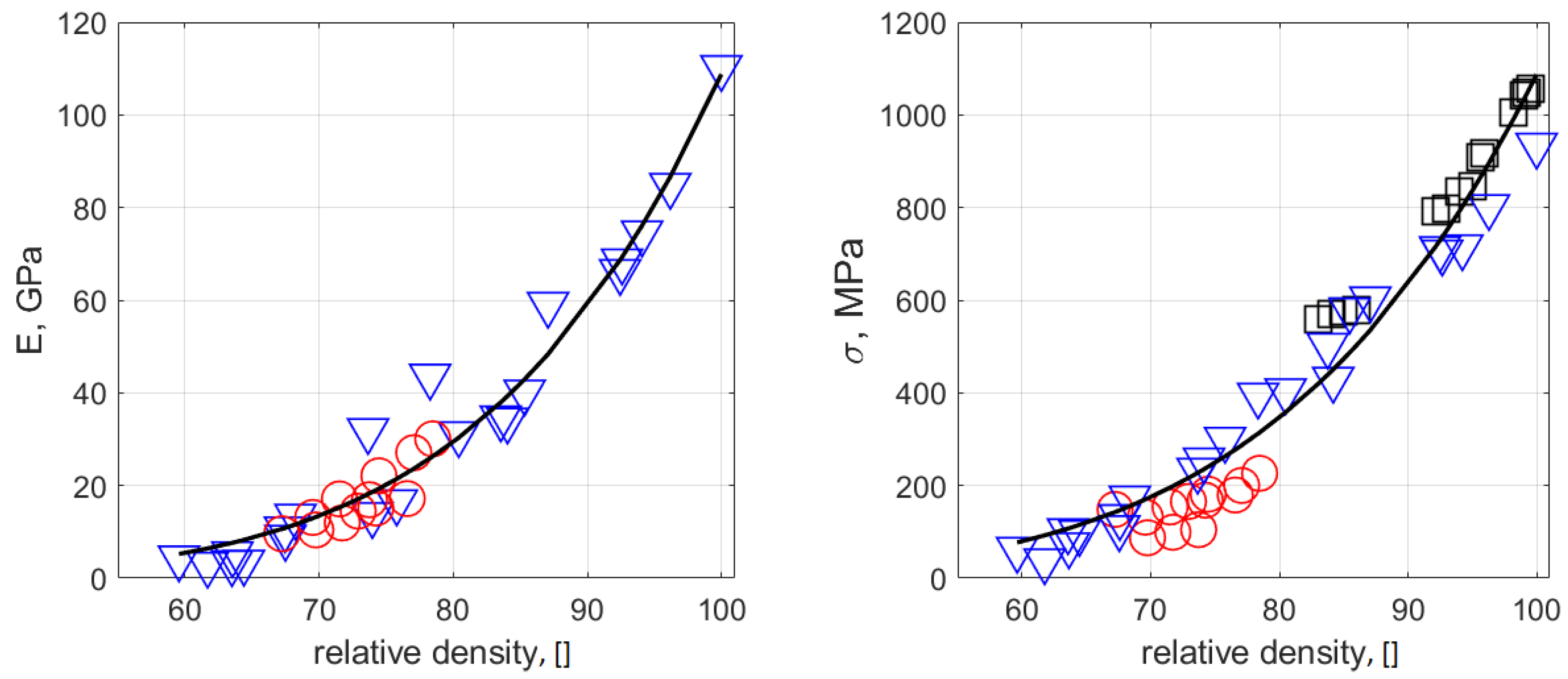
Section 5) was developed based on experimentally observed correlations, known mathematical results on packing densities, and analysis of shrinkage within the discrete element model. It was shown that the density of sintered samples is one of the key system parameters and can be correlated to the microstructure and mechanical properties of the samples. Accordingly, the simplified model assumes that, below threshold density ∼0.5, the metal powder during debinding behaves as a suspension of particles and demonstrates nonlinear shrinkage in the gravity direction. The lower the initial density the stronger the effect of gravity and hence nonlinearity. Above the threshold density the system behaves as a porous metal and shrinkage is nearly uniform. In microgravity, low initial density leads to agglomeration and a higher probability of faults. Therefore, to reduce the nonlinearity on the ground and improve the quality of the samples in microgravity, the initial density has to be as close as possible to the threshold value. The proposed mitigation strategies are based on the earlier experimental results and include e.g, using two-sized distribution to increase the initial powder density, reducing particle sizes, increasing sintering time, controlling the concentration of carbon and oxygen in the alloy, and controlling the binder system.
A full-scale finite element continuous model (
Section 6) of anisotropic shrinkage was developed in COMSOL
. Two macroscopic models were developed to describe the sintering process. One is based on the Olevsky approach and the other on thermal diffusion of backbone polymer. Both models demonstrate shrinkage of the initial structure of the whole part as a function of processing parameters. Both models predict nearly uniform shrinkage of the structure for high initial density and free boundary conditions. Anisotropic shrinkage was observed for spatial variation of the model parameters. It was shown that, besides gravity, fixed boundary conditions are an important factor of anisotropic shrinkage. The models can predict anisotropic shrinkage and determine the required compensation for the green part. The models depend on the number of phenomenological and experimental parameters that can be estimated with a developed multi-scale approach including sintering stress, diffusion coefficients, viscosity, etc.


 ,
, 


