Article

Parametric Study of Lateral Load on Helical Pipe Piles in Clay

1
School of Engineering and Built Environment, Griffith University, 58 Parklands Dr, Southport, QLD 4215, Australia
2
Blade Pile Group Pty., Ltd., 12 Junction Road, Burleigh Heads, Gold Coast, QLD 4220, Australia
*
Author to whom correspondence should be addressed.
Geotechnics 2024, 4(1), 158-179; https://doi.org/10.3390/geotechnics4010008
Submission received: 19 December 2023 / Revised: 12 January 2024 / Accepted: 18 January 2024 / Published: 19 January 2024

Abstract

:
In the past decades, as the world has placed emphasis on green energy, solar energy has become a favorable option. Different piled foundations have been designed to strengthen the structure supporting the solar panels. These piled foundations include rectangular and circular hollow section piles, as well as H-shaped piles. With various environmental loadings, lateral soil displacement will be encountered when large solar panels are installed on the supporting structure at an inclined angle. Presently, helical pipe piles are widely used in solar farms as part of the supporting structure. In this paper, the pile–soil interaction of steel pipe piles and helical pipe piles with wind loads is analyzed using ABAQUS. The Finite Element Method (FEM) models are assessed with varying strength moduli and cohesions of clay. Further, this paper examines the pile soil system, considering different clay stiffnesses, including very soft, soft, firm, stiff, very stiff, and hard. It is found that the helical piles’ horizontal capacity increases with soil strength and Young’s modulus, but the capacity increment rate reacts differently. This study has a guiding effect on the construction of solar farms using the “tracker” solar system.

Graphical Abstract

1. Introduction

1.1. Background

Nowadays, energy and environmental issues are among the most pressing challenges facing humanity, yet they remain difficult to resolve. Non-renewable energy sources are expensive to exploit and will eventually run out [1], so over-reliance on these sources is not a sustainable way to progress. The other issue in terms of the environment is global warming, which is caused primarily by the emission of greenhouse gases, especially carbon dioxide (CO2) [2]. It is reported that fossil fuel power generation and construction industries account for a large portion of the world’s CO2 emissions [3,4]. Therefore, developing clean energy solutions and improving emissions from the construction sector are crucial steps for countries to meet carbon emission standards.
Renewable energy accounted for about 29% of global electricity generation in 2020, according to the International Energy Agency’s (IEA) report on global electricity [3]. While this is a significant increase from previous years, it still represents a relatively small proportion of the world’s total electricity generation. Nevertheless, the growth in renewable energy is a positive sign and a highlight. As the demand for renewable energy continues to rise, photovoltaic solar power generation has become a promising area of development. However, constructing a solar farm requires special foundation systems to support the weight of the solar panels as well as lateral load action on these panels caused by wind.
H-shaped steel piles are commonly employed in modern solar farms as conventional pile structures. However, as highlighted by Rajapakse [
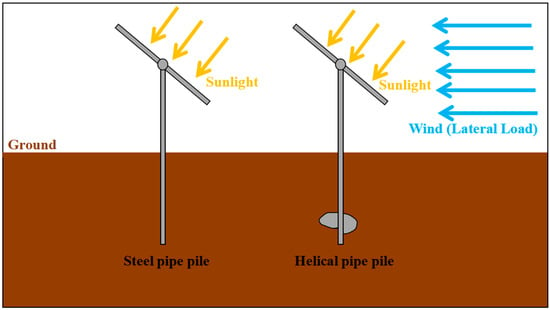
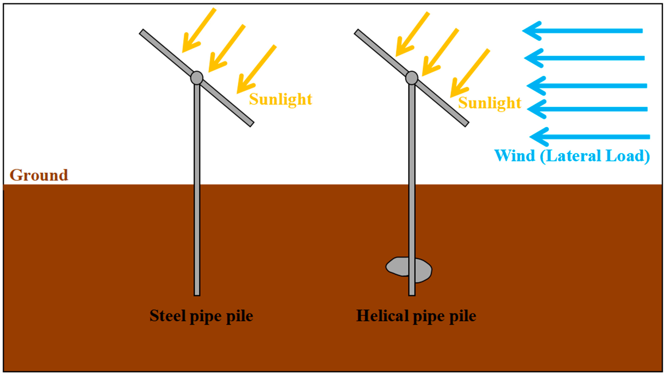
5], when H-shaped steel is “unplugged”, it has a small end bearing capacity but a large side friction, which is equivalent to a shaft resist pile. When subjected to lateral loads, their resistance mechanism predominantly depends on the flange area to counteract the lateral force. Nevertheless, the options for enhancing the horizontal capacity of H-shaped steel piles in the face of increased lateral loads are quite limited and costly. For instance, when increasing the flange width to improve the lateral capacity, the whole pile shafts will need to be increased, whereas only the top pile area requires such improvement, which will consequently lead to material waste and increased cost. In contrast, helical pipe piles offer a viable alternative by introducing a single helical plate to enhance the overall horizontal bearing capacity. The functioning principle of helical pipe piles is akin to that of an anchor, as they anchor into the soil, providing substantial bearing capacity. Consequently, the implementation of helical pipe piles offers a highly dependable solution, ensuring reliable bearing capacity while simultaneously minimizing material and financial wastage.
Spagnoli and de Hollanda Cavalcanti Tsuha [6] have emphasized the preference for helical pipe piles over ordinary piles in practical applications. These piles offer numerous advantages, including swift and noise-free installation, low maintenance requirements, and the ability to be easily installed in confined spaces and even on slopes. Additionally, helical piles exhibit convenient disassembly and reusability, making them highly versatile. They can be effectively employed in challenging scenarios with difficult water tables and deliver ample compression and tensile capacity [6,7,8,9,10,11]. Furthermore, Vignesh and Mayakrishnan [11] have highlighted the diverse applications of helical pipe piles, which include serving as uplift resistance in tunnel support systems, foundations for transmission towers, excavation support, and both land and offshore structures. Moreover, Vignesh and Mayakrishnan [11] consider helical pipe piles as an ideal and cost-effective choice for underwater structures, particularly for ensuring stability in submarine pipelines.
The use of screw piles or helical pipe piles can be traced back to 1838, when Alexander Mitchell employed them to support the Maplin Sands Lighthouse on the Thames [8]. However, the construction of helical pipe piles has faced significant challenges due to its intricate torsion-based construction method, impeding its development and research. The advent of hydraulic torque has brought attention to helical pipe piles and initiated preliminary research and development efforts [8].
Various computational methods have been developed to determine the pull and compressive capacity of helical pipe piles in cohesive and non-cohesive soils, including the individual method (b) and the cylindrical method [8,11,12,13,14]. Field tests conducted by Lutenegger [15] have yielded results consistent with the laboratory tests conducted by Rao and Prasad [16]. When the spacing ratio (SR), defined as the helical plate spacing divided by the helical plate diameter, is 1.5, it has been observed that the behavior of helical pipe piles exhibits individual plate bearing [17]. In soft to medium-hard clay, Rao et al. [17] determined that the optimal pull-out state of helical piles should have an SR value between 1 and 1.5. Hird and Stanier [18] found that when SR = 1.5, the compressive capacity of a pile with three helical plates was greater than that of a pile with one helical plate. Merifield [19] demonstrated that when SR is 1.58, the failure mechanism of helical piles transitions from cylindrical shear mode to single-board load mode.
Apart from the SR, there are many factors that may lead to changes in the bearing capacity of the helical pile, such as embedment ratios (H/D, the ratio of the depth between the top screw and the ground to the diameter of the top screw plate). Vignesh and Mayakrishnan [11] pointed out that the increase in H/D will increase the bearing capacity, but the research results of Merifield [19] showed that when H/D > 4, the increase in bearing capacity becomes less obvious. Trofimenkov and Mariupolskii [20] showed that the damage to the soil on the helical pile of a single helical plate depends on H/D, and the critical value of H/D refers to the depth of the helical plate that leads to the damage to the soil. Trofimenkov and Mariupolskii [20] obtained the critical value of H/D of the helical pile through experiments (H/D = 4–5 in clay; H/D = 5–6 in sand). Vignesh and Mayakrishnan [11] pointed out that when H/D > critical value of H/D, the damage to the helical pile will not cause surface uplift. In this case, the load is transferred from the pile to the soil through the helical plate and shaft, and the bearing capacity depends on the depth of the helical plate. When H/D < the critical value of H/D, the soil mass of the helical plate will bulge in the limit state. In addition, the research results of Nazir et al. [21] and El-Rahim et al. [7] also pointed out that the embedment depth of the helical plate would also affect its axial bearing capacity. Perko [8] suggested that the depth of the helical plate should be large enough, and placing the helical plate too close to the surface would cause shallow damage.
Merifield [19] highlighted the somewhat unsatisfactory state of current knowledge regarding the design of helical anchors, which has remained largely unchanged over the past two decades. Despite the increasing popularity of helical pipe piles in the field of engineering and the growing demand for screw piles, there remains an insufficient amount of research conducted on helical pipe piles. Consequently, there is a need for further studies to bridge these research gaps [11,22,23].
While Prasad and Rao [24] investigated the lateral load capacity of helical pipe piles and found that their horizontal bearing capacity was 1.2–1.5 times that of helical plate piles, Abdrabbo and Wakil [25] have emphasized the scarcity of research on helical pipe piles under lateral load. Several factors, including spiral plates, soil characteristics, diameter, number, and spacing of spiral blades, can influence the horizontal bearing capacity of helical pipe piles [25].
In the application of actual solar farms, helical piles have the advantages of high cost effectiveness, fast installation speed, strong tensile strength, environmental protection, etc., so they have been used in solar farms in Canada, the United States, and China to solve the problem of frost [26]. Sirivachiraporan and Wattanachannarong [27] also pointed out the use of helical piles in some solar farms in Thailand to improve carrying capacity. However, in the past application, the main purpose was to improve the axial bearing capacity through helical piles. Helical piles are ideal foundations for application in solar farms, and the application in solar farms has obvious capacity improvement [28]. However, Li et al. [12] pointed out in 2022 that the research on helical piles’ horizontal bearing capacity is limited and further research is needed. Therefore, to gain a better understanding of the horizontal capacity of helical pipe piles, this study conducted relevant research on the impact of soil parameters on helical pipe pile performance through numerical simulations utilizing ABAQUS (2022) software.

1.2. Research Purpose and Significance

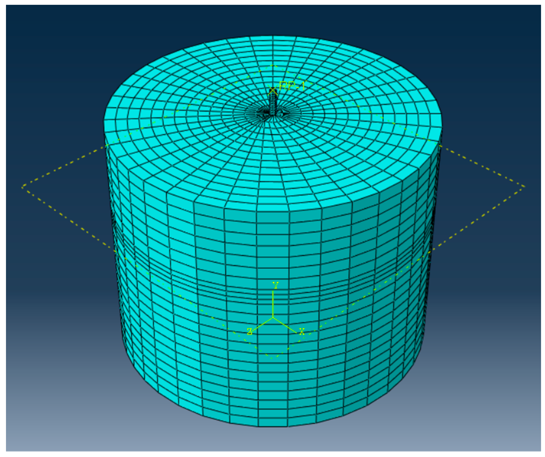
Previous research indicates that further investigation is necessary to gain a comprehensive understanding of helical piles and their potential applications. With the aim of providing robust support for the solar energy industry, this study seeks to analyze and compare the lateral ultimate bearing capacity of helical pipe piles and steel pipe piles in clay under horizontal load. To achieve this goal, the study will utilize ABAQUS software to conduct finite element analysis and simulate various types of clay’s geological conditions through numerical simulation.
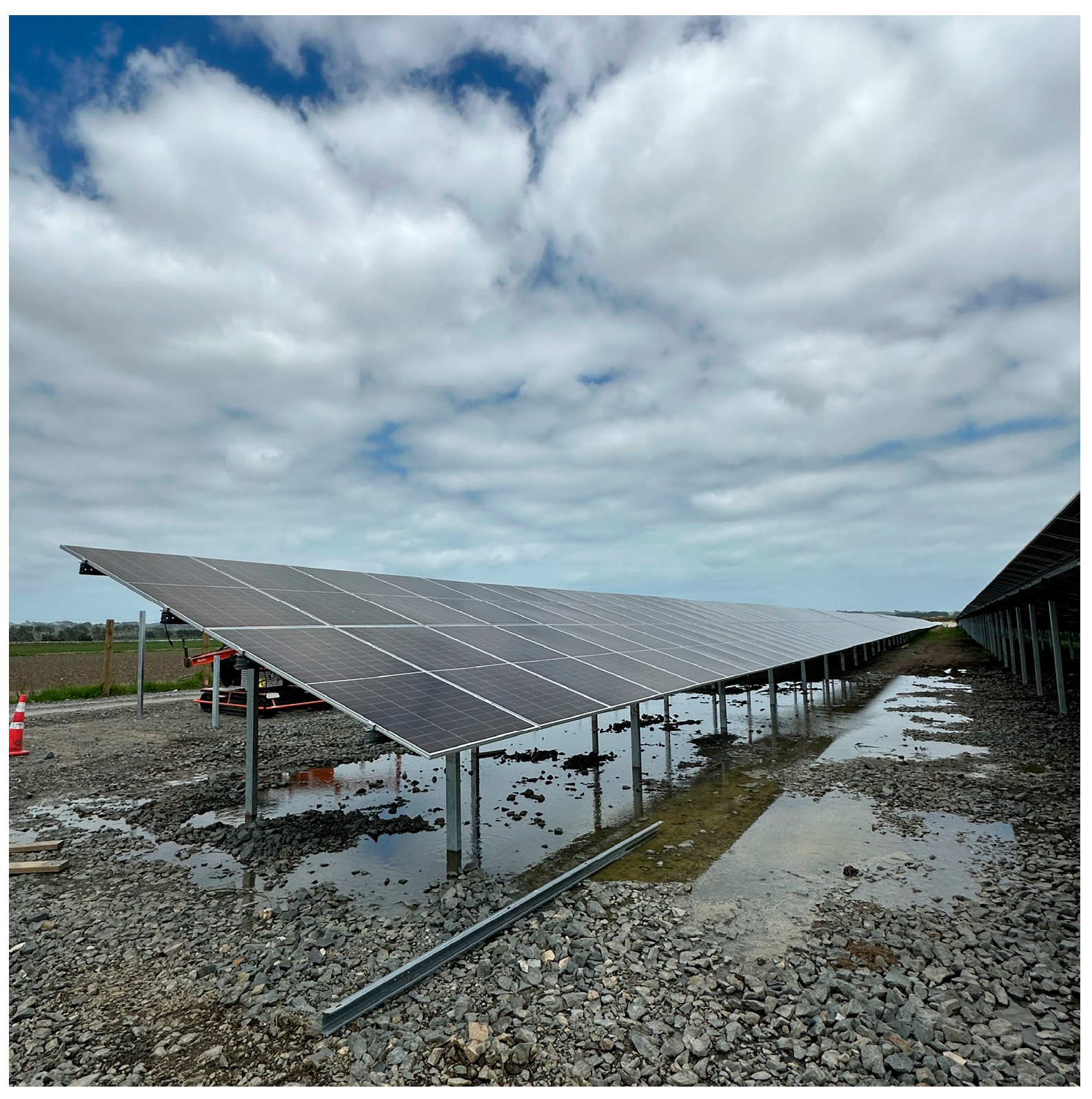
With the advancement of science and technology and the increasing global focus on clean energy, solar farms have found practical applications worldwide. Figure 1 depicts a conventional solar farm in New Zealand, where the solar panels are stationary and lack the ability to rotate. Observing the figure reveals that, due to this fixed orientation, the solar panels cannot consistently maintain optimal positioning as the sun’s position changes.
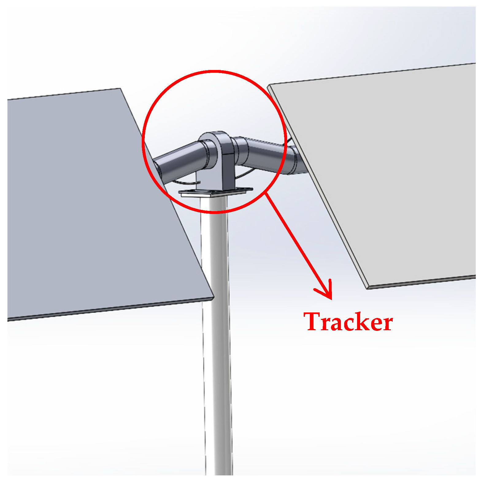
To enhance the efficiency of solar panels, a United States-based company has introduced an innovative solar system that employs a “tracker” mechanism to control panel rotation. This technology ensures that the solar panel plane maintains a vertical angle with sunlight by tracking the sun’s movement, as illustrated in Figure 2. The optimization of solar farms’ efficiency is achieved through precise control of the “tracker”. However, the ensuing problem is that when the rotation angle of the solar panel is too large, the contact area between the solar panel and the wind becomes larger, which requires a higher horizontal bearing capacity of the pile at the bottom of the solar panel.
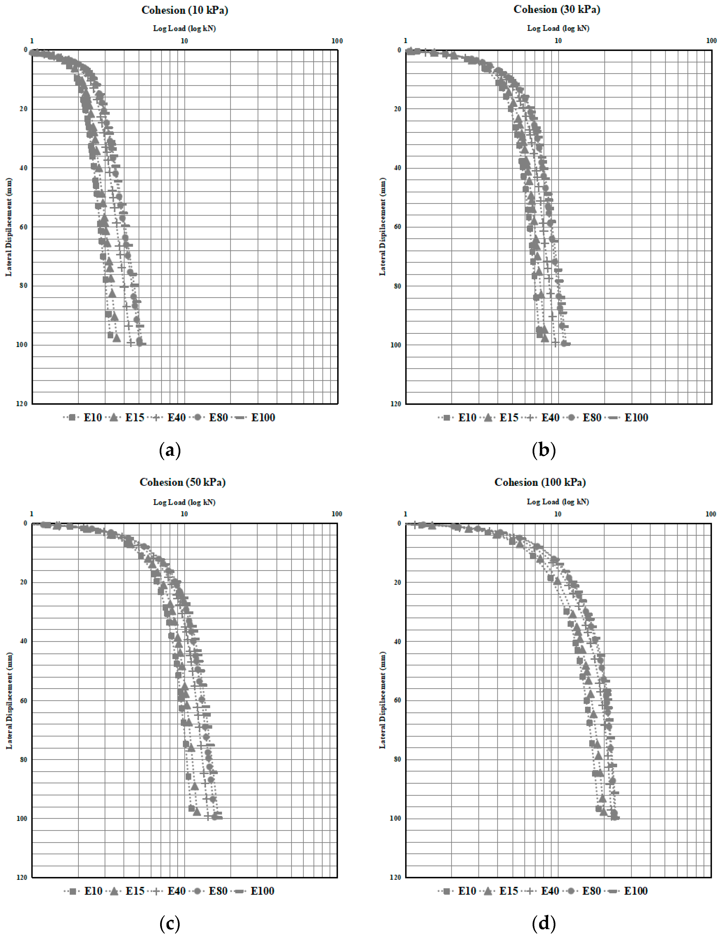
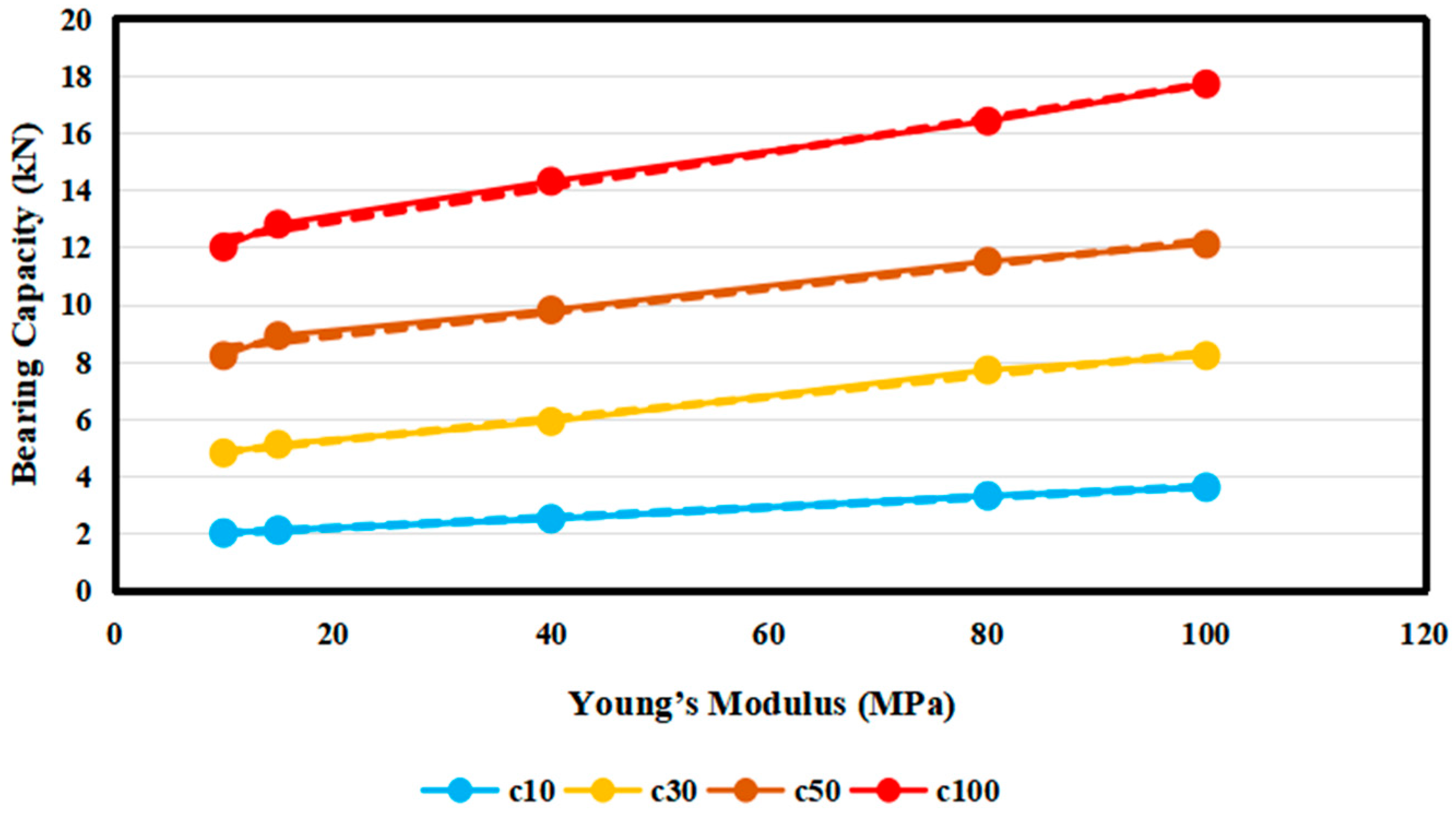
To promote the sustainable development of clean energy (solar energy), and the application and promotion of the “tracker” system, this paper compares two types of piles to investigate their lateral bearing capacity: one with a helical plate and the other without. Additionally, the study examines the effects of varying clay parameters on the Young’s modulus and cohesion of the soil.
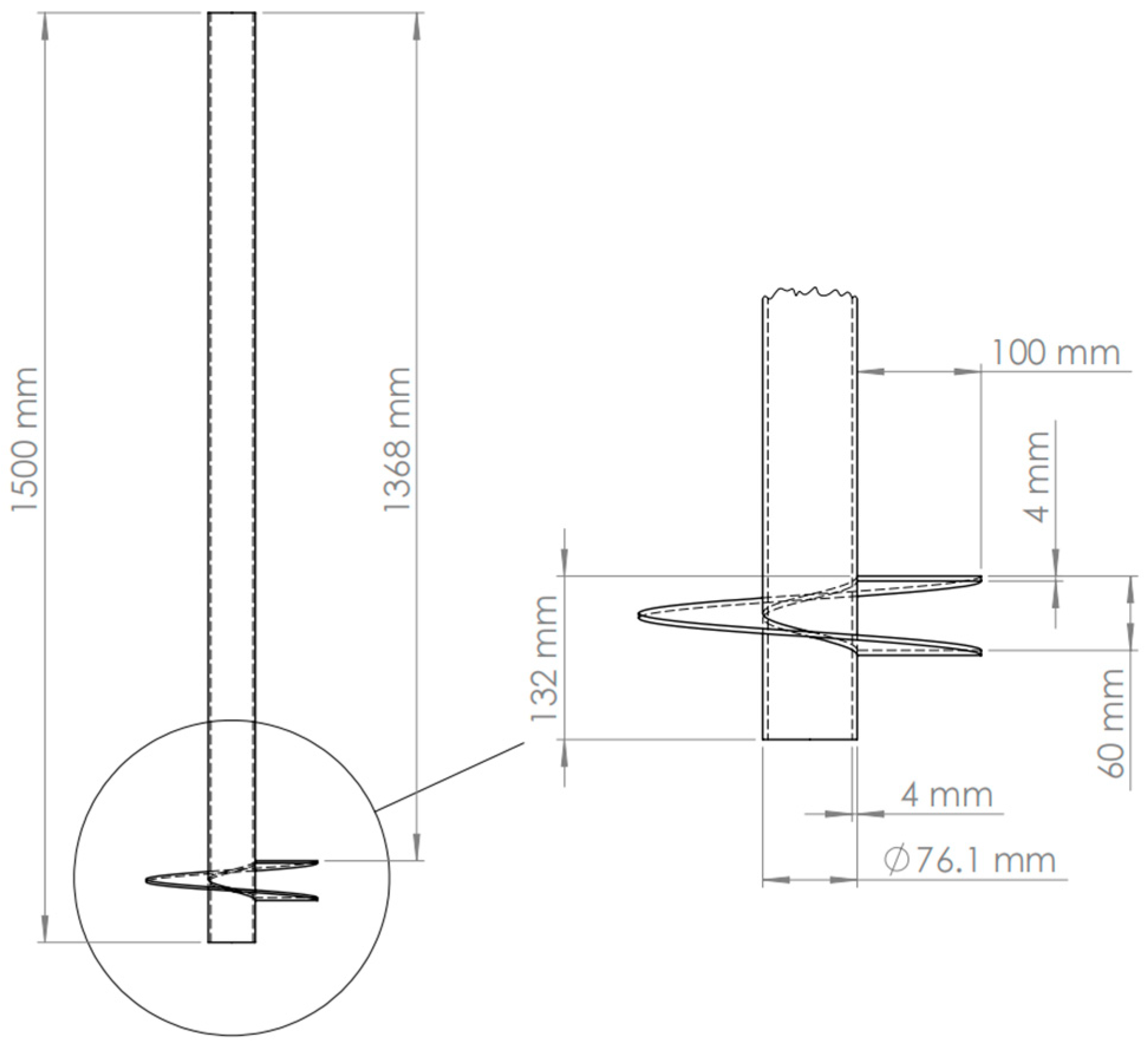
In consideration of material application in civil engineering, this study has selected a minimum standard outside diameter (O.D.) of 76.1 mm for piles. However, future research will also include larger O.D. piles available on the market as a variable for comparison.
Although helical pipe piles are becoming increasingly prevalent in the construction industry, their application scope remains limited worldwide. In light of this, this study seeks to showcase the advantages of helical pipe piles in enhancing horizontal ultimate bearing capacity through finite element analysis, building on current in-depth analysis and research into their applications in construction.

2. Parameter Setting for FEM Simulation of Piles

2.1. Parameters of Steel Pipe Pile and Helical Pipe Pile

Those pile structures with geometry variables can be dramatically different in relation to capacity. In detail, the helix added to those pile structures will change the stress path and, consequently, lead to differences in pile foundation loading capacity as well as the soil–pile stress mechanism. In this text, this research is only focused on the helix number, whereas the other parameters, which include outside diameter (O.D.), length of shaft (L), helix pitch (P), and thickness of the pile, were the same as 76.1 mm, 1500 mm, 60 mm, and 4 mm, respectively. It is worth noting that the size selected for this research project is the most widely used size in Australia, according to the survey, as summarized in Table 1.
As shown in Figure 3, the front view of the helical pipe pile and local enlargement of the helical plate are provided. This detailed drawing shows that the circle helix extends 100 mm; hence, the total enlarged pile end achieves 276.1 mm. The minimum thickness of the helical plate in this research is 4 mm. Moreover, the helical plate pitch is 60 mm. It is worth noting that the distance between the top of the helical plate and the top of the helical pile is 1368 mm (i.e., from the top of the helical plate to the pile tip: 132 mm). The reason for setting the helical plate at this position is to ensure that the middle of the helical plate is 100 mm away from the bottom of the helical pipe pile.
For the comparison research between steel pipe piles and helical pipe piles, the steel material grade is the same. Based on the AS 4100 [29], the yield and ultimate strength of G450 are 450 and 520 MPa, respectively. The other steel parameters between these two types of piles are also the same, which include Young’s modulus, Poisson’s ratio, and density with values of 210 GPa, 0.3, and 7.8 × 10⁻⁹ t/mm3, respectively.
As for the clay soil research, the considered parameter is mainly focused on the effect of Young’s modulus as well as soil strength of cohesion, and the detailed values are provided in Table 2 and Table 3. As depicted in Table 2, to research Young’s modulus effect on lateral pile capacity, cohesion will be maintained from 10 to 100 kPa, whereas the modulus will increase from 10 to 100 MPa. As shown in Table 3, the modulus will be maintained, and the cohesion values will include 10, 20, 30, 50, 80, and 100 MPa in numerical simulation to examine the lateral behavior of piles.
In this study, the above-selected soil parameters were numerically simulated to make up for the shortcomings of previous studies focusing on individual soils. Through a systematic parameter study, this study studied the theoretical manifestation of all possible combinations of soil parameters. In addition, numerical simulation of several real clay conditions in Section 2.2 has been performed to provide powerful guidance and reference for practical applications.

2.2. Real Clay State of Steel Pipe Pile and Helical Pipe Pile

The parametric study can provide an empirical correlation between the soil parameters and pile lateral capacity, but it may be unreal. The limitation of the parametrical study is that the FEM simulation is idealized. In fact, the soil cohesion will increase with modulus. Owing to increased credibility to reflect the real soil state, extra FEM models are created to investigate the helical piles, and the detailed soil parameters are covered in Table 4. As shown in this table, six types of clay are included, which consist of very soft (v.soft), soft, firm, stiff, very stiff (v.stiff), and hard. Note that the soil strength classification referenced is based on Table 5.3 of Look [30].

2.3. Model Setup for FEM Numerical Simulation

The constitutive relationship for FEM simulation between these two types of piles is the same as the Mohr–Coulomb relationship. Also, the mesh seeding is kept the same. Based on the recommendation proposed by Li et al. (2022) [12], the soil boundary dimension to be considered will be 20 times the target structure, at least in terms of the x, y, and z directions. In this study, a 4 m O.D. and 3 m deep soil column is established for FEM simulation (4 m/76.1 > 20; 3 m/1.5 < 20). Although the depth of the column soil does not reach 20 times that of the pile, this study mainly focuses on the horizontal bearing capacity of the helical pile, so the influence on depth is not great, as shown in Figure 4.
In this study, the model was calculated using Mohr-Coulomb criteria. The calculation results of ABAQUS were summarized in EXCEL, and Li et al. (2022) [12] adopted the same method to find the point of sharp increase in displacement through the logarithmic method and calculated the ultimate bearing capacity and displacement of the pile foundation. In the process of making the model, first determine the size of the model, make the model, and then set the parameters of the model. In the setting of model parameters, this study first sets the properties of helical pile and soil (modifying different properties of helical pile and soil according to the research content). Then, it sets the load position of the model, the calculation steps of ABAQUS, the boundary conditions, and the friction coefficient, and, finally, carries out the grid division.
This study focuses on horizontal capacity. Therefore, the most important thing in setting boundary conditions is to fix the soil around it so that it cannot move horizontally and the bottom of the soil cannot rotate or move in any direction. Considering the dead weight generated by the upper and middle objects in practice, the dead weight of the solar panel is set to be 9.8 kN in this study. In addition, in this study, the shape of the grid is mainly divided into two types: a tetrahedral grid and a hexahedral grid. Among them, the hexahedral grid with both pile body and soil is set, and the tetrahedral grid with a helical plate is set due to its irregular shape. In addition, the setting of the mesh size is also very important. The mesh size of the soil in this study is about 140, and that of the helical pile is about 30. It is worth mentioning that the flip bias ratio was not set for mesh seeding in this study, but the seed number of soil around the helical plate was increased. The mesh size changes in a small range depending on the model. In this study, the number of units in the helical pile is roughly 1150, and the number of units in the soil is roughly 18,300. The number of cells will vary a little from model to model because the mesh sizes set up for better convergence and computation will vary a little. In addition, it is worth mentioning that the friction coefficient of contact between soil and helical pile in this study is set at 0.3. In addition, Figure 4 shows the mesh image of the FEM model.

3. Parametrical Study of Steel Pipe Piles and Helical Pipe Piles

3.1. Numerical Simulation Results of Steel Pipe Piles

3.1.1. Effect of Young’s Modulus in Steel Pipe Piles

When soil cohesion is 10, 30, 50, and 100 MPa, respectively, the lateral displacement versus corresponding loads of steel pipe piles in soil with different Young’s moduli is provided in Figure 5a–d respectively. Moreover, in order to distinguish the influence of different Young’s moduli on steel pipe piles, different marks (such as a square, triangle, etc.) were set for different Young’s moduli in Figure 5a–d. In this figure, it can be seen that under the same condition of cohesion, the changes in Young’s modulus affected the behavior of the soil steel pipe pile foundation. In detail, with Young’s modulus increasing, the maximum loads resisted by the steel pipe pile became greater.
Three stages of the behavior of steel pipe piles are found in all plotted displacements versus log loads. The first stage shows linear behavior, and in the second stage, soil plasticity starts, but at a low rate. The last stage demonstrates the failure condition due to dramatic displacement being found. In this paper, by finding two tangent lines from stages 1 and 3, the intersection represents the ultimate bearing capacity and corresponding ultimate displacement of the steel pipe pile.
The horizontal ultimate bearing capacity of the steel pipe pile, interpreted from Figure 5, is summarized in Table 5. As shown in Table 5, the lateral capacity increases with Young’s modulus when soil cohesion is invariable at 10, 30, 50, and 100 MPa. For example, when the soil cohesion for the FEM model is at 10 MPa with increasing Young’s modulus, the ultimate lateral capacity increases accordingly. To find the capacity increment rate (slope of capacity/Young’s modulus) of the steel pipe pile, Young’s modulus versus capacity was plotted in Figure 6. This figure also shows the same outcome, which is that the lateral capacity increases with Young’s modulus. Furthermore, this figure represents that the rate among slopes is not the same; with a slope discovered to have of a cohesion of 100 kPa, Young’s modulus has a greater bearing capacity.

3.1.2. Effect of Cohesion in Steel Pipe Pile

Young’s modulus is set as the invariant to research the effect of cohesion on horizontal ultimate bearing capacity. Young’s modulus is considered invariant, i.e., 30, 50, 80, and 100 MPa, whereas the variable of cohesion ranges from 10 to 120 kPa. By changing the variable parameter of cohesion, the load versus displacements of soil when Young’s modulus is 30, 50, 80, and 100 MPa are presented in Figure 7a–d, respectively.
The distance between the two curves (such as cohesion, which is equal to 10 and 120 kPa, respectively) presents the effect of cohesion or Young’s modulus on bearing capacity. For example, in Figure 5a, Young’s modulus increases from 10 to 100 kPa, and the capacity improves from 2.0 to 3.6 kN (increased by 1.6 kN). As can be seen from Figure 7a, the capacity improves by 13.8 kN from 2.1 to 15.9 kN, and compared with Figure 5a, cohesion has a greater impact on the horizontal ultimate bearing capacity of steel pipe pile than Young’s modulus. In detail, the log load of different cohesions changes more, as shown in Figure 7a–d.
The capacity of soil with different values of Young’s modulus and cohesion is summarized in Table 6. Note that the capacity of these piles is obtained by interpreting log load versus displacement curves from Figure 7a–d. It can be seen from Table 6 that when the value of Young’s modulus (E) is fixed, the ultimate bearing capacity of the steel pipe pile increases with the increase in cohesion. For instance, when Young’s modulus was 30 MPa, by comparing the pile capacity of cohesion to 10 to 120 kPa, the horizontal ultimate bearing capacity of steel pipe pile was determined to be 2.1 to 15.9 kN, respectively, which has increased by 657%. Furthermore, when Young’s modulus was 50, 80, and 100 MPa, the horizontal bearing capacity increased by 562%, 455%, and 442%, respectively. It can be seen that with the growth of Young’s modulus, cohesion has a smaller impact on the growth rate of bearing capacity.
To assess the cohesion effect on capacity, the cohesion versus capacity diagram is plotted in Figure 8, and the trend equation and slope of the relationship between bearing capacity and cohesion are obtained by making a trend line. As shown in this figure, there is a relatively obvious boundary: when the cohesion is less than 50 kPa, slopes a, b, c, and d equal 0.2, 0.2043, 0.2046, and 0.212, respectively; when the cohesion is more than 50 kPa, slopes A, B, C, and D equal 0.0838, 0.0931, 0.0973, and 0.1069, respectively. The slope of the curves represents the capacity improvement rate; the horizontal axis is cohesion; and the vertical axis represents bearing capacity. Moreover, for cohesion less than 50 kPa, the horizontal bearing capacity improvement is greater, and after 50 kPa, there is less effect because the average slope is 0.0953. However, when cohesion is less than 50 kPa, it is 0.2052.
According to the ultimate bearing capacity shown in Figure 8, it can be seen that there is a positive correlation between cohesion and the ultimate bearing capacity (Qult) of steel pipe piles, as shown in Equation (1).
Q u l t Δ y x C
where: Qult = Ultimate bearing capacity of steel pipe pile in clay; Δ y x = 0.2052 (10 ≤ C ≤ 50); =0.0953 (50 < C ≤ 120); C = Cohesion of clay.

3.2. Numerical Simulation Results of Helical Pipe Pile

3.2.1. Effect of Young’s Modulus on Helical Pipe Pile

To better reflect the response influence of Young’s modulus on the horizontal ultimate bearing capacity of helical pipe pile, several Young’s modulus values were set (10, 15, 40, 80, and 100 MPa, respectively), and the value of cohesion was fixed at 10, 30, 50, and 100 kPa. The numerical simulation results, which represent the relationship between log load and displacement, are shown in Figure 9a–d. As can be seen from this figure, the increase in the Young’s modulus value will lead to an increase in the ultimate bearing capacity of the helical pipe pile when cohesion is a constant value.
According to the analysis of the log load versus displacement curves in Figure 9a–d, the horizontal ultimate bearing capacity of the helical pipe pile is summarized in Table 7. As can be seen from this table, when cohesion is fixed, the horizontal bearing capacity of the helical pipe pile increases with the growth of Young’s modulus. In detail, by changing the Young’s modulus from 10 to 100 MPa, the capacity increased to 5.8, 10.8, 15.7, and 21.9 kN when the cohesion constant was 10, 30, 50, and 100 kPa, respectively. This table also shows the improvement percentage of the capacity of the helical pipe pile. To illustrate, when cohesion was 10 kPa, Young’s modulus increased from 10 to 100 MPa, and the horizontal ultimate bearing capacity of the helical pipe pile increased by 70.59% (from 3.4 to 5.8 kN). Furthermore, when cohesion was 30, 50, and 100 kPa, the horizontal ultimate bearing capacity of the helical pipe pile increased by 42.11%, 40.18, and 32.73% kN (from 7.6 to 10.8 kN; 11.2 to 15.7 kN; and 16.5 to 21.9 kN, respectively).
To research the capacity improvement rate, the capacity increment rate (slope of capacity/Young’s modulus) of the helical pipe pile is plotted in Figure 10, in which the slopes of the curves c10, c30, c50, and c100 represent the capacity increment rate. Further, the four curves show different slopes (0.0243, 0.0346, 0.0459, and 0.0585), which infer a cohesion increase will lead to an increase in the capacity increment rate. It is worth mentioning that the four slopes are obtained by four trend lines and best-fit equations.

3.2.2. Effect of Cohesion in Helical Pipe Pile

To study the effect of cohesion on the horizontal ultimate bearing capacity of the helical pipe pile, six cohesion values were set, which are 10, 20, 30, 50, 100, and 120 kPa. The numerical simulation results of the log load and displacement relationship are arranged in Figure 11a–d. It can be seen from this figure that cohesion had a significant impact on the horizontal ultimate bearing capacity of the helical pipe pile.
The horizontal bearing capacity of the helical pipe pile is summarized in Table 8. It can be seen from this table that clay cohesion had a great influence on the horizontal ultimate bearing capacity of the helical pipe pile. Case in point: when Young’s modulus was 30 MPa and cohesion was 10 kPa and 120 kPa, the horizontal ultimate bearing capacity of the helical pipe pile was 3.9 kN and 20.8 kN, respectively, and it was increased by 433.33%. Moreover, when Young’s modulus was 50, 80, and 100 MPa, the horizontal ultimate bearing capacity of the helical pipe pile increased by 386.67%, 354%, and 305.17%, respectively.
To better reflect the response, the horizontal bearing capacity of the helical pipe pile increases significantly with the increase in cohesion, as plotted in Figure 12. Note that the changing trend of the horizontal ultimate bearing capacity was divided into two stages, with 50 kPa cohesion as the intermediate point. In the first stage, when the cohesion is less than 50 kPa, the growth rate of bearing capacity changes more obviously with cohesion than in the second stage.
Similar to the finding of steel pipe piles, there was a positive correlation between the horizontal ultimate bearing capacity (Qult-helical) of helical pipe piles and clay cohesion (C), as proposed in Equation (2). However, the difference is the slope (0.2375, 10  C  50 kPa; 0.1163, 50 < C ≤ 120 kPa). It should be mentioned that the trendline equation in Figure 12 is for a clearer observation of the slope.
Q u l t h e l i c a l Δ y x C
where: Qult-helical = Ultimate bearing capacity of helical pipe pile in clay; Δ y x = 0.2375 (10 kPa ≤ C ≤ 50 kPa); =0.1163 (50 kPa < C ≤ 120 kPa); C = Cohesion of clay.

3.3. Comparison between the Steel Pile and Helical Pipe Pile

A reasonable comparison of the influence of Young’s modulus on the horizontal ultimate bearing capacity of steel pipe piles and helical pipe piles is plotted in Figure 13a–d. In this figure, the cohesion value has four fixed values of 10, 30, 50, and 100 kPa. To explore the influence of Young’s modulus, it was set at 10, 15, 40, 80, and 100 MPa. The blue curves in the figure represent the relationship between the log load and displacement of the helical pipe pile, while the red curves correspond to the steel pipe pile. The difference in bearing capacity between steel pipe pile and helical pipe pile under the same conditions can be more clearly observed, which is that the horizontal bearing capacity of helical pipe pile under the influence of Young’s modulus is significantly higher than that of steel pipe pile, as shown in Figure 13a–d.
According to the log load versus displacement curves in Figure 13a–d, the horizontal bearing capacity of the steel pipe pile and helical pipe pile is summarized in Table 9. This table shows that the bearing capacity of the helical pipe pile is greater than that of the steel pipe pile. In detail, when cohesion is 10 kPa and Young’s modulus is 10 and 100 MPa, respectively, the bearing capacity of the helical pipe pile is 1.4 and 2.2 kN greater than that of the steel pipe pile, respectively.
Furthermore, the bearing capacity range of steel pipe piles and helical pipe piles increases with the increase in cohesion. For instance, when cohesion increases from 10 to 100 kPa and Young’s modulus increases from 10 to 100 MPa, the capacity range of the steel pipe pile increases from 1.6 kN to 5.7 kN; similarly, the helical pipe pile has a capacity range from 2.4 kN to 5.4 kN.
In order to compare the difference in the influence of cohesion on the bearing capacity of steel pipe piles and helical pipe piles, Figure 14a–d are plotted. In this figure, the blue curves represent the relationship between the log load and displacement of the helical pipe pile, and the red curves indicate steel pipe piles. It can be clearly seen from this figure that the bearing capacity of helical pipe piles is greater than that of steel pipe piles under the influence of cohesion.
According to the relationship between log load and displacement in Figure 14a–d, the ultimate bearing capacity of the steel pipe pile and helical pipe pile is sorted out in Table 10. In this table, c10 and c120 represent cohesions of 10 and 120 kPa, respectively. It is observed that the capacity range of steel pipe piles and helical pipe piles has improved as Young’s modulus increases. When Young’s modulus goes from 30 to 100 MPa, the capacity range of the steel pipe pile and helical pipe pile increases from 13.8 and 16.9 kN to 15.9 and 17.7 kN, respectively.
Moreover, the increment in capacity is shown in this table, and the capacity of the helical pipe pile is higher than that of the steel pipe pile. Note that when the value of Young’s modulus is fixed, the cohesion value is 120 kPa, and the bearing capacity of the helical pipe pile will increase much more than when the cohesion value is 10 kPa. To illustrate, when Young’s modulus is 30 MPa, the cohesion is 120 and 10 kPa, respectively, and the corresponding increment in bearing capacity is 4.9 and 1.8 kN.
In addition, according to the results of the cohesion influence on steel pipe piles and helical pipe piles, relevant rules of slope (capacity/cohesion) change were found and are summarized in Table 11. When cohesion was less than 50 kPa, the slope (capacity/cohesion) of the helical pipe pile increased by 15.74% compared with that of the steel pipe pile. However, when it was greater than 50 kPa, the slope (capacity/cohesion) grew more, increasing by 22.04%.

4. Comparison of the Real Clay State Regarding Steel Pipe Pile and Helical Pipe Pile

To avoid overly idealized clay parameter simulation, the numerical simulation of the real clay state is carried out, and the attending simulation results are shown in Figure 15 below. Six different clay situations are set for the real clay state, which is very soft, soft, firm, stiff, very stiff, and hard. As can be seen from Figure 15, there are obvious differences between the bearing capacity of helical pipe piles and steel pipe piles, namely that the bearing capacity of the helical pipe pile is greater than that of the steel pipe pile, regardless of the clay type. Note that the legend in this table is composed of three parts: the type of piles, including the degree of softness and hardness of clay, Young’s modulus, and cohesion. To illustrate, “S-V.Soft-E10c10” and “H-Soft-E15c15” stand for “steel pipe pile-very soft clay-10 MPa of Young’s modulus and 10 kPa of cohesion” and “helical pipe pile-soft clay-15 MPa of Young’s modulus and 15 kPa of cohesion”, respectively.
According to the relationship between log load and displacement in Figure 15, the horizontal bearing capacity of the helical pipe pile and steel pipe pile was arranged in Table 12. As can be seen in this table, the horizontal bearing capacity of helical pipe piles is greater than that of steel pipe piles in all types of clay. Furthermore, with the increase in clay hardness, the increased percentage of ultimate bearing capacity of the helical pipe pile decreases. Specifically, compared with steel pipe piles, the horizontal ultimate bearing capacity of very soft to hard helical pipe piles was increased by 70%, 54.84%, 35.94%, 31.62%, 26.37%, and 23.66%, respectively.
To more clearly compare the bearing capacity of steel pipe piles and helical pipe piles in a real clay state, Figure 16 was plotted. For the helical pipe pile and steel pipe pile, the increasing trend of bearing capacity in clay can be divided into three stages in this figure. Moreover, the slopes (growth rate of bearing capacity) of the three stages are different, as shown in Figure 16. The slopes of stages I and III are both smaller than those of stage II, which means that the bearing capacity of piles increases more slowly in stages I and III than in stage II. Furthermore, the capacity difference between helical pipe pile and steel pipe pile is different in the three stages, which are a (1.7 kN), b (4.3 kN), and c (5.3 kN). It is worth noting that these three differences represent the lifting effect of the capacity of the helical pipe pile compared with that of the steel pipe pile. It was in stage III (very stiff and hard clay) that the capacity boost from the helical pipe pile worked best, as shown in Figure 16.

5. Conclusions and Recommendations

Although relevant studies on helical pipe piles have been carried out in the past, these investigations were mostly focused on the compression loading conditions in different types of soil. Studies on the horizontal bearing capacity of the helical pipe piles are extremely lacking. By FEM numerical simulation of helical piles in clay, a parametrical study was performed. The effect of Young’s modulus and soil strength parameters was investigated, and the following was concluded:
  • When values of cohesion are fixed, the capacity of steel as well as helical pipe piles both increase with the Young’s modulus. The capacity improvement or increment rate is very close.
  • When Young’s modulus value is fixed, both circular tube piles and helical pipe piles increase with the increase in the cohesion parameter; however, the capacity increment rate is different. It was found that 50 kPa is the boundary value. In detail, when soil cohesion is greater than 50 kPa, the horizontal bearing capacity of both piles increases at a smaller rate with the increase in cohesion. The increment rate (slope gradient) for both types of piles is proposed.
The load versus soil lateral displacement were analyzed and compared considering soil cohesion and Young’s modulus between 10 kPa and 100 kPa and between 10 MPa and 120 MPa, respectively. The following was found:
  • Helical piles show better results than steel pipe piles in the same type of soil.
  • Both types of piles demonstrate better capacity when the soil strength parameter is increased. But the capacity increment range is different; the helical pile capacity increment with that specific geometry is greater than that of a normal steel pipe pile.
This paper also studies the pile behavior under lateral loads, which shows various states. Six types of clay soil are included (very soft, soft, firm, stiff, very stiff, and hard), and the following is concluded:
  • The pile capacity of both types of piles will be greater when they are installed in good-strength soil. The greater increment rate for both types of piles is found when piles are installed in firm to very stiff soil.
  • By adding a helix to the pipe pile and installing it in very stiff to hard clay, the pile capacity under the specific geometry shows a greater value of 5.3 kN (Figure 16).
It is worth mentioning that there are still some limitations to this study, as follows:
  • This study only considers the theoretical results under ideal conditions.

Author Contributions

The numerical simulation method employed in this study was proposed by J.Z., who holds the patent for Blade Pile Group Pty Ltd. For the sake of convenience in future research and comparison, this study only examined steel pipe piles without helical plates and helical pipe piles with a single helical plate. The finite element model was developed by G.S. under the supervision of E.O., while the writing and editing of this article were conducted by G.S. and J.Z. Progress management was overseen by G.S. and E.O., with data analysis conducted by all authors listed in this article. Additionally, G.S. and L.L. conducted chart review. All authors have read and agreed to the published version of the manuscript.

Funding

This research received no external funding.

Data Availability Statement

The data presented in this study are available on request from the corresponding author. The data are not publicly available due to ethical.

Acknowledgments

Thanks to all the authors for their contributions, as well as to Blade Pile Group Pty Ltd. for their invaluable support.

Conflicts of Interest

As the corresponding author of the manuscript, Jialin Zhou is from Blade Pile Group Pty., Ltd. He participated in the writing of the manuscript and provided the numerical simulation method for this study. The authors declare no conflicts of interest.

References

  1. Hart, R. Non-renewable resources in the long run. J. Econ. Dyn. Control 2016, 71, 1–20. [Google Scholar] [CrossRef]
  2. Meinshausen, M.; Meinshausen, N.; Hare, W.; Raper SC, B.; Frieler, K.; Knutti, R.; Frame, D.J.; Allen, M.R. Greenhouse-gas emission targets for limiting global warming to 2 °C. Nature 2009, 458, 1158–1162. [Google Scholar] [CrossRef] [PubMed]
  3. International Energy Agency. Global Electricity Review 2021; International Energy Agency: Paris, France, 2021; p. 15. Available online: https://www.iea.org/reports/global-electricity-review-2021 (accessed on 19 October 2023).
  4. Shaikh, F.U.A.; Vimonsatit, V. Compressive strength of fly-ash-based geopolymer concrete at elevated temperatures. Fire Mater. 2015, 39, 174–188. [Google Scholar] [CrossRef]
  5. Rajapakse, R.A. Pile Design and Construction Rules of Thumb; Butterworth-Heinemann: Oxford, UK, 2016. [Google Scholar]
  6. Spagnoli, G.; de Hollanda Cavalcanti Tsuha, C. A review on the behavior of helical piles as a potential offshore foundation system. Mar. Georesour. Geotechnol. 2020, 38, 1013–1036. [Google Scholar] [CrossRef]
  7. El-Rahim, A.; Hamdy, H.A.; Taha, Y.K. The compression and uplift bearing capacities of helical piles in cohesionless soil. J. Eng. Sci. 2013, 41, 2055–2064. [Google Scholar] [CrossRef]
  8. Perko, H.A. Helical Piles: A Practical Guide to Design and Installation; Wiley: Hoboken, NJ, USA, 2009. [Google Scholar] [CrossRef]
  9. Livneh, B.; El Naggar, M.H. Axial testing and numerical modeling of square shaft helical piles under compressive and tensile loading. Can. Geotech. J. 2008, 45, 1142–1155. [Google Scholar] [CrossRef]
  10. Sakr, M. Performance of helical piles in oil sand. Can. Geotech. J. 2009, 46, 1046–1061. [Google Scholar] [CrossRef]
  11. Vignesh, V.; Mayakrishnan, M. Design parameters and behavior of helical piles in cohesive soils—A review. Arab. J. Geosci. 2020, 13, 1194. [Google Scholar] [CrossRef]
  12. Li, L.; Sui, G.; Zhou, J.; Oh, E. Parametric Study of Lateral Loaded Blade Pile in Clay. Geosciences 2022, 12, 329. [Google Scholar] [CrossRef]
  13. Nasr, M. Performance-based design for helical piles. In Proceedings of the Contemporary Topics in Deep Foundations, Orlando, FL, USA, 15–19 March 2009; pp. 496–503. [Google Scholar] [CrossRef]
  14. Mohajerani, A.; Bosnjak, D.; Bromwich, D. Analysis and design methods of screw piles: A review. Soils Found. 2016, 56, 115–128. [Google Scholar] [CrossRef]
  15. Lutenegger, A.J. Cylindrical shear or plate bearing?—Uplift behavior of multi-helix screw anchors in clay. In Proceedings of the Contemporary Topics in Deep Foundations, Orlando, FL, USA, 15–19 March 2009; pp. 456–463. [Google Scholar]
  16. Rao, S.N.; Prasad, Y.V.S.N.; Veeresh, C. Behaviour of embedded model screw anchors in soft clays. Geotechnique 1993, 43, 605–614. [Google Scholar] [CrossRef]
  17. Rao, S.N.; Prasad, T.V.S.N.; Shetty, M.D. The behaviour of model screw piles in cohesive soils. Soils Found. 1991, 31, 35–50. [Google Scholar] [CrossRef] [PubMed]
  18. Hird, C.C.; Stanier, S.A. Modelling helical screw piles in clay using a transparent soil. In Proceedings of the 7th International Conference on Physical Modelling in Geotechnics, Zurich, Switzerland, 27 June 2010–2 July 2010; Volume 6. [Google Scholar]
  19. Merifield, R.S. Ultimate uplift capacity of multiplate helical type anchors in clay. J. Geotech. Geoenviron. Eng. 2011, 137, 704–716. [Google Scholar] [CrossRef]
  20. Trofimenkov, J.G.; Mariupolskii, L.G. Screw piles used for mast and tower foundations. In Proceedings of the 6th International Conference on Soil Mechanics and Foundation Engineering, Montreal, QC, Canada, 8–15 September 1965. [Google Scholar]
  21. Nazir, R.; Chuan, H.S.; Niroumand, H.; Kassim, K.A. Performance of single vertical helical anchor embedded in dry sand. Meas. J. Int. Meas. Confed. 2014, 49, 42–51. [Google Scholar] [CrossRef]
  22. Pack, J.S. Design of helical piles for heavily loaded structures. In Proceedings of the New Technological and Design Developments in Deep Foundations, Denver, CO, USA, 5–8 August 2000; pp. 353–367. [Google Scholar]
  23. Perlow, M., Jr. Helical pile acceptance criteria, design guidelines, and load test verification. In Proceedings of the Geo-Frontiers 2011: Advances in Geotechnical Engineering, Dallas, TX, USA, 13–16 March 2011; pp. 94–102. [Google Scholar]
  24. Prasad, Y.V.S.N.; Rao, S.N. Lateral capacity of helical piles in clays. J. Geotech. Eng. 1996, 122, 938. [Google Scholar] [CrossRef]
  25. Abdrabbo, F.; El Wakil, A. Laterally loaded helical piles in sand. Alex. Eng. J. 2016, 55, 3239–3245. [Google Scholar] [CrossRef]
  26. Wang, T.; Liu, J.; Luo, Q.; Wang, Q.; Zhang, L.; Qi, W. Calculation for frost jacking resistance of single helical steel piles in cohesive soils. J. Cold Reg. Eng. 2021, 35, 06021001. [Google Scholar] [CrossRef]
  27. Sirivachiraporan, A.; Wattanachannarong, C. The using of ground screw pile as mounting structure foundation in solar PV farm. In Proceedings of the International Congress on Engineering and Information, Osaka, Japan, 10–12 May 2016. [Google Scholar]
  28. Feng, S.J.; Fu, W.D.; Chen, H.X.; Li, H.X.; Xie, Y.L.; Lv, S.F.; Li, J. Field tests of micro screw anchor piles under different loading conditions at three soil sites. Bull. Eng. Geol. Environ. 2021, 80, 127–144. [Google Scholar] [CrossRef]
  29. AS 4100:2020; Steel Structures. Standards Australia: Sydney, Australia, 2000.
  30. Look, B. Handbook of Geotechnical Investigation and Design Tables, 2nd ed.; CRC Press: Boca Raton, FL, USA, 2014. [Google Scholar] [CrossRef]
Figure 1. A typical solar farm.
Geotechnics 04 00008 g001
Figure 2. Solar panel system with tracker.
Geotechnics 04 00008 g002
Figure 3. Sectional view of the helical pipe pile with an enlarged view highlighting the diameter, thickness of the pile, and helix pitch.
Geotechnics 04 00008 g003
Figure 4. Mesh image of the FEM model.
Geotechnics 04 00008 g004
Figure 5. Lateral displacement of steel pipe piles: (a) cohesion of 10 kPa; (b) cohesion of 30 kPa; (c) cohesion of 50 kPa; (d) cohesion of 100 kPa.
Geotechnics 04 00008 g005
Figure 6. Relationship between Young’s modulus and the ultimate bearing capacity of the steel pipe pile.
Geotechnics 04 00008 g006
Figure 7. Lateral displacement of steel pipe piles (a) Young’s modulus of 30 MPa; (b) Young’s modulus of 50 MPa; (c) Young’s modulus of 80 MPa; (d) Young’s modulus of 100 MPa.
Geotechnics 04 00008 g007
Figure 8. Relationship between cohesion and ultimate bearing capacity of the steel pipe pile.
Geotechnics 04 00008 g008
Figure 9. Lateral displacement of helical pipe piles: (a) cohesion of 10 kPa; (b) cohesion of 30 kPa; (c) cohesion of 50 kPa; (d) cohesion of 100 kPa.
Geotechnics 04 00008 g009
Figure 10. Relationship between Young’s modulus and the bearing capacity of the helical pipe pile.
Geotechnics 04 00008 g010
Figure 11. Lateral displacement of helical pipe piles (a) Young’s modulus of 30 MPa; (b) Young’s modulus of 50 MPa; (c) Young’s modulus of 80 MPa; (d) Young’s modulus of 100 MPa.
Geotechnics 04 00008 g011
Figure 12. Relationship between cohesion and ultimate bearing capacity of the helical pipe pile.
Geotechnics 04 00008 g012
Figure 13. Lateral displacement of helical pipe piles and steel pipe piles: (a) cohesion of 10 MPa; (b) cohesion of 30 MPa; (c) cohesion of 50 MPa; (d) cohesion of 100 MPa.
Geotechnics 04 00008 g013
Figure 14. Lateral displacement of helical pipe piles and steel pipe piles: (a) Young’s modulus of 30 MPa; (b) Young’s modulus of 50 MPa; (c) Young’s modulus of 80 MPa; (d) Young’s modulus of 100 MPa.
Geotechnics 04 00008 g014aGeotechnics 04 00008 g014b
Figure 15. Performance of the steel pipe pile and the helical pipe pile in clay.
Geotechnics 04 00008 g015
Figure 16. Helical pipe pile bearing capacity enhancement effect.
Geotechnics 04 00008 g016
Table 1. Geometric parameters of steel pipe pile and helical pipe pile.
Geometric ParametersSteel Pipe PileHelical Pipe Pile
Outside Diameter (mm)76.176.1
Length of Shaft (mm)15001500
Thickness of the Pile (mm)44
Helix Pitch (mm)N/A60
Number of Helical Plates01
Table 2. The controlled parameter—soil cohesion.
Soil Cohesion (kPa)Young’s Modulus (MPa)
c = 10E = 10, 15, 40, 80 and 100
c = 30E = 10, 15, 40, 80 and 100
c = 50E = 10, 15, 40, 80 and 100
c = 100E = 10, 15, 40, 80 and 100
Table 3. The controlled parameter—Young’s modulus.
Young’s Modulus (MPa)Soil Cohesive (kPa)
E = 15c = 10, 20, 30, 50, 80 and 100
E = 40c = 10, 20, 30, 50, 80 and 100
E = 80c = 10, 20, 30, 50, 80 and 100
E = 100c = 10, 20, 30, 50, 80 and 100
Table 4. Real soil state of clay.
Soil TypeUnit Weight (γ), kN/m3Soil Cohesion (c), kPaYoung’s Modulus (E), MPa
V.Soft161010
Soft171515
Firm183030
Stiff198080
V.Stiff19.5150150
Hard20200200
Table 5. Effect of Young’s modulus on the ultimate bearing capacity of the steel pipe pile.
Cohesion (kPa)Young’s Modulus (MPa)
10154080100
Ultimate Bearing Capacity (kN)
c = 10 kPa2.02.12.53.33.6
c = 30 kPa4.85.15.97.78.2
c = 50 kPa8.28.99.811.512.1
c = 100 kPa12.012.814.316.417.7
Table 6. Cohesion effect on the ultimate bearing capacity of the steel pipe pile.
Young’s Modulus (MPa)Cohesion (kPa)
10154080100120
Ultimate Bearing Capacity (kN)
E = 30 MPa2.14.26.410.114.515.9
E = 50 MPa2.64.86.910.815.817.2
E = 80 MPa3.35.57.711.516.418.3
E = 100 MPa3.65.98.212.117.719.5
Table 7. Effect of Young’s modulus on the ultimate bearing capacity of the helical pipe pile.
Cohesion (kPa)Young’s Modulus (MPa)
10154080100
Ultimate Bearing Capacity (kN)
c = 10 kPa3.43.74.35.05.8
c = 30 kPa7.68.08.910.210.8
c = 50 kPa11.211.913.214.515.7
c = 100 kPa16.517.319.221.221.9
Table 8. Cohesion effect on the ultimate bearing capacity of the helical pipe pile.
Young’s Modulus (MPa)Cohesion (kPa)
10154080100120
Ultimate Bearing Capacity (kN)
E = 30 MPa3.96.28.713.319.220.8
E = 50 MPa4.56.99.413.620.421.9
E = 80 MPa5.07.510.214.521.222.7
E = 100 MPa5.88.110.815.721.923.5
Table 9. Comparison of the ultimate bearing capacity range (cohesion).
Cohesion (kPa)Steel Pipe PileHelical Pipe PileIncremental (kN)
E10 to E100RangeE10 to E100RangeE10E100
Ultimate Bearing Capacity (kN)
c = 10 kPa2.0–3.61.63.4–5.82.41.42.2
c = 30 kPa4.8–8.23.47.6–10.83.22.82.6
c = 50 kPa8.2–12.13.911.2–15.74.53.63.6
c = 100 kPa12.0–17.75.716.5–21.95.44.24.2
Table 10. Comparison of the ultimate bearing capacity range (Young’s modulus).
Young’s Modulus (MPa)Steel Pipe PileHelical Pipe PileIncremental (kN)
c10 to c120Rangec10 to c120Rangec10c120
Ultimate Bearing Capacity (kN)
E = 30 MPa2.1–15.913.83.9–20.816.91.84.9
E = 50 MPa2.6–17.214.64.5–21.917.41.94.7
E = 80 MPa3.3–18.315.05.0–22.717.71.74.4
E = 100 MPa3.6–19.515.95.8–23.517.72.24.0
Table 11. The effect of cohesion on the steel pipe pile and the helical pipe pile.
Slope (Capacity/Cohesion)
10 ≤ C ≤ 50 (kPa)50 < C ≤ 120 (kPa)
Steel pipe pile0.20520.0953
Helical pipe pile0.23750.1163
Increments and Percentages15.74%22.04%
Table 12. Comparison of the ultimate bearing capacity of steel pipe pile and helical pipe pile.
Ultimate Bearing Capacity (kN)
V.SoftSoftFirmStiffV.StiffHard
E10-c10E15-c15E30-c30E80-c80E150-c150E200-c200
Steel pipe pile2.03.16.413.620.122.4
Helical pipe pile3.44.88.717.925.427.7
Increase (%)70.0054.8435.9431.6226.3723.66
Disclaimer/Publisher’s Note: The statements, opinions and data contained in all publications are solely those of the individual author(s) and contributor(s) and not of MDPI and/or the editor(s). MDPI and/or the editor(s) disclaim responsibility for any injury to people or property resulting from any ideas, methods, instructions or products referred to in the content.

