Elastic Solutions to 2D Plane Strain Problems: Nonlinear Contact and Settlement Analysis for Shallow Foundations

Abstract

The classical Neumann boundary value problem of an isotropic, homogeneous elastic half-plane under plane strain conditions is readdressed as the limiting case of the fully three-dimensional problem. Analytical solutions of the stress and strain tensors are obtained by taking the limit from known three-dimensional solutions. It is shown that the displacement fields for the plane strain problem are not well defined. A small number of simple expressions are developed, which provide a general solution for linearly-varying traction over arbitrary regions on the boundary. A simple, efficient, and rapidly convergent algorithm is developed which uses these solutions as analytic elements and provides a solution approach to the general boundary value problem. The method is verified against known solutions for Hertzian contact between parallel cylinders. Two numerical examples are presented for the analysis of shallow foundation systems. In the first, the boundary conditions are informed by analytical elastoplastic calculations and a strain influence analysis is performed and compared with the Schmertmann method. Subsequently, empirical laboratory contact traction distributions measured by Bauer et al., in both the normal and tangential directions are employed as boundary conditions for an analysis of the underlying stress field.

1. Introduction

The problem of an isotropic and homogeneous elastic half-plane under plane strain with given conditions on its linear boundary has been well-studied for over a century. Various equivalent open-form integral solutions have been obtained for the Neumann problem, where the distributions of boundary traction are prescribed. The problem was first solved by Flamant [1] for concentrated point forces; boundary integral representations of the stress and strain fields under distributed traction can be obtained by making use of the classical Flamant solution as a fundamental solution (e.g., [2]). Alternatively, the solutions can be obtained directly from the governing equations using Fourier transforms [3] or by manipulating potentials in the complex domain [4,5]. Analytical closed-form solutions of these fields, which are easy to evaluate at any point of interest in the material domain, are available only for a select few, simple cases of interest [2,4].

The plane strain problem in linear elasticity has a history of application in the analysis of soil-structure interaction problems. The assumptions that the out of plane strain is zero is suitable for long strip foundations, allowing for analysis of only the center line of contact with the underlying soil and reducing the problem to from three to two dimensions. There are clear limitations to representing a granular soil body as an isotropic and homogeneous linear-elastic solid. The approach represents perhaps the most extreme simplification, in which the complex interaction of discrete grains are homogenized by a representative elastic continuum. However, the ability to solve for closed-form expressions has made elastic solutions very attractive for quick approximations of the stress, strain, and settlement of foundation systems. Boussinesq, who pioneered the earliest closed-form solutions for boundary value problems [6], also wrote explicitly about the mechanics of granular soils decades before soil mechanics were properly formulated in the early 20th century [7]. Later, when Love calculated some of the first closed-form solutions for distributed normal tractions, he framed his work as “an attempt to throw some light on the important technical question of the safety of foundations [8]”. These fundamental elastic solutions became the foundation of many methods assessing the equilibrium and settlement of shallow foundation systems. Newmark used these solutions as the basis of his popular stress influence method, providing graphical charts to aid in engineering calculations [9]. The famous strain influence method of Schmertmann [10,11] is similarly based on tabulated values of the strain fields calculated in an elastic half-space. More recent works continue to use fundamental calculations from linear elasticity to assess the settlement of foundation systems [12,13,14,15,16,17]. This list is far from exhaustive.

Recent work [18] has suggested that using physically-accurate boundary conditions (that represent the stress states between footings and real granular materials) can import some of the nonlinear behavior due to the discrete granular assembly into the linear elastic analysis. This approach may lead to a better representation of the stress and strain fields within the loaded elastic body representing an underlying soil. In order to conveniently study the behavior of these fields and their dependence on the boundary data for the plane strain case, mathematical tools are required to represent them (at least approximately) within the half-plane. This could be achieved through either direct analytical or numerical integration of the known open-form integral solutions. The former approach is tedious or intractable for boundary traction fields of arbitrary complexity. On the other hand, point-wise numerical integration of the boundary integrals can be computationally expensive and prohibits an in-depth study of the behavior of stress and strain fields under evolving boundary conditions.

The present paper provides simple analytical tools for the representation of the tensor field solutions for the Neumann plane strain problem. New simplified closed-form solutions are presented for low-order monomial boundary conditions; these are obtained by taking analytic limits from known closed-form solutions of the 3D problem [16,17]. Surprisingly, a relatively small number of simple analytical expressions are found to completely determine the problem. These expressions are then applied as analytic elements to form continuous approximate solutions to higher-order and arbitrary boundary conditions. Applications to geotechnical problems of soil–structure interaction are then presented, which involve analytical and empirical boundary data.

2. Methodology

2.1. Plane Strain as a Limit of the Fully Three-Dimensional Half-Space Problem

Recent work has been done to provide analytical closed-form solutions for the elastic stress, strain, and displacement fields on a fully three-dimensional isotropic and homogeneous elastic half-space under polynomial Neumann boundary conditions [16,17,19,20]. Consider the half-space ${\mathbb{H}}^3=\{(x,y,z)\in {\mathbb{R}}^3|z>0\}$ as described by the three-dimensional Cartesian coordinate system shown in Figure 1. For static conditions without body forces, the solid is ultimately governed by the system of elliptic partial differentials equations [21]:

$$\begin{array}{cc}\hfill & (\lambda +\mu )\frac{\partial D}{\partial x}+\mu \Delta u=0\hfill \\ \hfill & (\lambda +\mu )\frac{\partial D}{\partial y}+\mu \Delta v=0\hfill \\ \hfill & (\lambda +\mu )\frac{\partial D}{\partial z}+\mu \Delta w=0.\hfill \end{array}$$

(1)

Here $\lambda ,\mu$ are the Lamé elastic constants, $(u,v,w)$ are the elastic displacements in the Cartesian $(x,y,z)$ directions, $D=\frac{\partial u}{\partial x}+\frac{\partial v}{\partial y}+\frac{\partial w}{\partial z}$ is the strain dilation, and $\Delta =\frac{{\partial }^2}{\partial x^2}+\frac{{\partial }^2}{\partial y^2}+\frac{{\partial }^2}{\partial z^2}$ is the Laplacian differential operator. The problem is defined when boundary traction functions $q_x,q_y,p$ are prescribed (acting in the $x,y$, and z directions, respectively) over a subset $R\subset \partial {\mathbb{H}}^3$. The half-space boundary $\partial {\mathbb{H}}^3$ consists of the points in the plane $z=0$, and R can in general be the union of any disjoint subsets, outside of which the boundary conditions are assumed to be zero. It is also assumed that the displacements, and consequently the strains and stresses, go to zero as distance from the source region R becomes large.

Based originally on the work of Boussinesq [6] and Cerruti [22], the displacement, stress, and strain fields under monomial traction distributions of order $m,n$ can be constructed from three potential functions from ${\mathbb{H}}^3\to \mathbb{R}$:

$$\begin{array}{cc}\hfill & A^{mn}=\underset{R}{\int \int }\frac{{\left(x^{\prime }\right)}^m{\left(y^{\prime }\right)}^n}{r}d{x}^{\prime }d{y}^{\prime }\hfill \end{array}$$

(2)

$$\begin{array}{cc}\hfill & B^{mn}=\underset{R}{\int \int }{\left(x^{\prime }\right)}^m{\left(y^{\prime }\right)}^{n}log\left(z+r\right)d{x}^{\prime }d{y}^{\prime }\hfill \end{array}$$

(3)

$$\begin{array}{cc}\hfill & {\mathsf{\Gamma }}^{mn}=\underset{R}{\int \int }{\left(x^{\prime }\right)}^m{\left(y^{\prime }\right)}^n[zlog(z+r)-r]d{x}^{\prime }d{y}^{\prime },\hfill \\ \hfill & r=\sqrt{{(x^{\prime }-x)}^2+{(y^{\prime }-y)}^2+z^2}\hfill \end{array}$$

(4)

The superscripts $mn$ on the three-dimensional potentials (2)–(4) correspond to the order of the boundary conditions given spatially by monomial terms ${\left(x^{\prime }\right)}^m{\left(y^{\prime }\right)}^n$. These functions satisfy the three-dimensional Laplace equation, i.e., $\Delta A^{mn}=\Delta B^{mn}=\Delta {\mathsf{\Gamma }}^{mn}=0$. It is also relevant to note that the three functions $A^{mn},B^{mn}$, and ${\mathsf{\Gamma }}^{mn}$ are not fully independent but are related by the following differential operations:

$$\begin{array}{cc}\hfill & B^{mn}=\frac{\partial {\mathsf{\Gamma }}^{mn}}{\partial z},\hfill \\ \hfill & A^{mn}=\frac{\partial B^{mn}}{\partial z}=\frac{{\partial }^2{\mathsf{\Gamma }}^{mn}}{\partial z^2}.\hfill \end{array}$$

2.1.1. Calculation Approach

The potentials corresponding to the plane strain problem can be obtained from Equations (2)–(4) by taking limits as one dimension of the boundary region R becomes infinite. Let $R=\{(x,y)\in \partial {\mathbb{H}}^3|a_2\le x\le a_1,-b\le y\le b\}$, such that the integrals in Equations (2)–(4) are taken over a rectangle centered at the origin in the y-direction but which lies on an arbitrary cut of the x-axis. Geometrical intuition assures us that as b becomes arbitrarily large, the potentials will exhibit less dependence on the spatial variable y; as b becomes infinite, every y value, having infinite length of rectangle to either side of it, becomes equivalent. This also corresponds to the intuitive geometrical definition of plane strain problems. The potentials which solve the elastic plane strain problem in the $xz$-plane for monomial boundary traction fields varying with x can formally be defined as:

$$\begin{array}{cc}\hfill & \frac{{\partial }^{j+k}{A}^m}{\partial x^j\partial z^k}=\underset{b\to \infty }{lim}\frac{{\partial }^{j+k}{A}^{m0}}{\partial x^j\partial z^k}=\underset{b\to \infty }{lim}\frac{{\partial }^{j+k}}{\partial x^j\partial z^k}{\int }_{-b}^b{\int }_{a_2}^{a_1}\frac{{\left(x^{\prime }\right)}^m}{r}d{x}^{\prime }d{y}^{\prime }\hfill \\ \hfill \end{array}$$

(5)

$$\begin{array}{cc}\hfill & \frac{{\partial }^{j+k}{B}^m}{\partial x^j\partial z^k}=\underset{b\to \infty }{lim}\frac{{\partial }^{j+k}{B}^{m0}}{\partial x^j\partial z^k}=\underset{b\to \infty }{lim}\frac{{\partial }^{j+k}}{\partial x^j\partial z^k}{\int }_{-b}^b{\int }_{a_2}^{a_1}{\left(x^{\prime }\right)}^{m}log\left(z+r\right)d{x}^{\prime }d{y}^{\prime }\hfill \\ \hfill \end{array}$$

(6)

$$\begin{array}{cc}\hfill & \frac{{\partial }^{j+k}{\mathsf{\Gamma }}^m}{\partial x^j\partial z^k}=\underset{b\to \infty }{lim}\frac{{\partial }^{j+k}{\mathsf{\Gamma }}^{m0}}{\partial x^j\partial z^k}=\underset{b\to \infty }{lim}\frac{{\partial }^{j+k}}{\partial x^j\partial z^k}{\int }_{-b}^b{\int }_{a_2}^{a_1}{\left(x^{\prime }\right)}^m[zlog(z+r)-r]d{x}^{\prime }d{y}^{\prime }.\hfill \end{array}$$

(7)

Here, $j,k$ are simply the (integer) orders of the $x,z,$ partial derivatives, respectively. As will be shown below, these expressions do not converge to well-defined limit functions for some values (e.g., $j=k=0$). However, the derivatives required to define the stress and strain tensors (see [16,17]) are all well-defined. All partial derivatives with respect to the y variable tend to zero in the limit, while the convergent functions (5)–(7) are independent of y.

The analytical properties discussed earlier for Equations (2)–(4) (namely that they satisfy the Laplace equation and are interrelated via differentiation) all hold in the limit for Equations (5)–(7). The following identities can be derived:

$$\begin{array}{cc}\hfill & \frac{{\partial }^3{\mathsf{\Gamma }}^m}{\partial x^3}=-\frac{\partial A^m}{\partial x}\hfill \\ \hfill & \frac{{\partial }^3{B}^m}{\partial x^3}=-\frac{{\partial }^2{A}^m}{\partial x\partial z}\hfill \\ \hfill & \frac{{\partial }^2{B}^m}{\partial x^2}=-\frac{\partial A^m}{\partial z}\hfill \\ \hfill & \frac{{\partial }^2{A}^m}{\partial x^2}=-\frac{{\partial }^2{A}^m}{\partial z^2}\hfill \end{array}$$

The result is that the stress and strain tensors for the plane strain problem can be completely determined by only four potential functions for each case, expressible in terms of Equation (5) alone.

The stress component fields when the normal traction is $p\left(x^{\prime }\right)={\left(x^{\prime }\right)}^m$ and the tangential traction $q\left(x^{\prime }\right)=0$ are obtained from those for three-dimensional problem given in [16] and are listed as follows:

$$\begin{array}{cc}\hfill & {\left({\sigma }_{xx}\right)}_p^m=\frac{1}{2\pi }\left(\frac{\partial A^m}{\partial z}+z\frac{{\partial }^2{A}^m}{\partial z^2}\right)\hfill \\ \hfill \end{array}$$

(8)

$$\begin{array}{cc}\hfill & {\left({\sigma }_{yy}\right)}_p^m=\frac{1}{2\pi }\left(\frac{\lambda }{\lambda +\mu }\frac{\partial A^m}{\partial z}\right)\hfill \\ \hfill \end{array}$$

(9)

$$\begin{array}{cc}\hfill & {\left({\sigma }_{zz}\right)}_p^m=\frac{1}{2\pi }\left(\frac{\partial A^m}{\partial z}-z\frac{{\partial }^2{A}^m}{\partial z^2}\right)\hfill \\ \hfill \end{array}$$

(10)

$$\begin{array}{cc}\hfill & {\left({\sigma }_{xz}\right)}_p^m=-\frac{1}{2\pi }\left(z\frac{{\partial }^2{A}^m}{\partial x\partial z}\right)\hfill \end{array}$$

(11)

The superscript m again indicates the order of the monomial boundary traction, while the subscript p indicates the direction of the nonzero traction component for Equations (8)–(11). The shearing components in the y plane are zero everywhere, i.e., ${\left({\sigma }_{yz}\right)}_p^m={\left({\sigma }_{xy}\right)}_p^m=0$. It is clear from the above expressions that the strain component ${\left({ϵ}_{yy}\right)}_p^m$ vanishes by Hooke’s law. The out-of-plane stress ${\left({\sigma }_{yy}\right)}_p^m$ is a finite non-zero function of the x and z coordinates due to Poisson’s effect. Note that in general, under plane strain conditions, all stress components besides ${\sigma }_{yy}$ are independent of the elastic constants of the material. Poisson’s effect yields the dependence

$$\begin{array}{c}\hfill {\sigma }_{yy}=\frac{\lambda }{2(\lambda +\mu )}({\sigma }_{xx}+{\sigma }_{zz})=\nu ({\sigma }_{xx}+{\sigma }_{zz})\end{array}$$

Thus, the stress tensor is dependent only on the boundary conditions and the Poisson ratio $\nu$.

The stress components for the case where tangential boundary traction is $q\left(x^{\prime }\right)={\left(x^{\prime }\right)}^m$ and the normal traction $p\left(x^{\prime }\right)=0$ are given as follows:

$$\begin{array}{cc}\hfill & {\left({\sigma }_{xx}\right)}_q^m=\frac{1}{2\pi }\left(2\frac{\partial A^m}{\partial x}+z\frac{{\partial }^2{A}^m}{\partial x\partial z}\right)\hfill \\ \hfill \end{array}$$

(12)

$$\begin{array}{cc}\hfill & {\left({\sigma }_{yy}\right)}_q^m=\frac{1}{2\pi }\left(\frac{\lambda }{\lambda +\mu }\frac{\partial A^m}{\partial x}\right)\hfill \\ \hfill \end{array}$$

(13)

$$\begin{array}{cc}\hfill & {\left({\sigma }_{zz}\right)}_q^m=-\frac{1}{2\pi }\left(z\frac{{\partial }^2{A}^m}{\partial x\partial z}\right)\hfill \\ \hfill \end{array}$$

(14)

$$\begin{array}{cc}\hfill & {\left({\sigma }_{xz}\right)}_q^m=\frac{1}{2\pi }\left(\frac{\partial A^m}{\partial z}-z\frac{{\partial }^2{A}^m}{\partial z^2}\right)\hfill \end{array}$$

(15)

The components of Equations (12)–(15) can be superimposed with those of Equations (8)–(11) to obtain the stress fields for plane strain boundary value problems with nonzero $p\left(x^{\prime }\right)$ and $q\left(x^{\prime }\right)$.

The required partial derivatives of Equations (2)–(4) are known in closed-form for constant and linear traction fields; the potentials required to satisfy (8)–(15) can be obtained by direct calculation from these closed-form solutions by taking a limit as in Equation (5). For example, it is shown in [16] that for the rectangular region R defined here,

$$\begin{array}{cc}\hfill \frac{\partial A^{10}}{\partial z}& =\frac{\partial }{\partial z}{\int }_{-b}^b{\int }_{a_2}^{a_1}\frac{x^{\prime }}{r}d{x}^{\prime }d{y}^{\prime }\hfill \\ \\ \hfill & =\left(zlog\left(\sqrt{{(a_1-x)}^2+{(b-y)}^2+z^2}+b-y\right)-x{tan}^{-1}\left(\frac{(a_1-x)(b-y)}{z\sqrt{{(a_1-x)}^2+{(b-y)}^2+z^2}}\right)\right)\hfill \\ \\ \hfill & -\left(zlog\left(\sqrt{{(a_1-x)}^2+{(-b-y)}^2+z^2}-b-y\right)-x{tan}^{-1}\left(\frac{(a_1-x)(-b-y)}{z\sqrt{{(a_1-x)}^2+{(-b-y)}^2+z^2}}\right)\right)\hfill \\ \\ \hfill & -\left(zlog\left(\sqrt{{(a_2-x)}^2+{(b-y)}^2+z^2}+b-y\right)-x{tan}^{-1}\left(\frac{(a_2-x)(b-y)}{z\sqrt{{(a_2-x)}^2+{(b-y)}^2+z^2}}\right)\right)\hfill \\ \\ \hfill & +\left(zlog\left(\sqrt{{(a_2-x)}^2+{(-b-y)}^2+z^2}-b-y\right)-x{tan}^{-1}\left(\frac{(a_2-x)(-b-y)}{z\sqrt{{(a_2-x)}^2+{(-b-y)}^2+z^2}}\right)\right)\hfill \end{array}$$

By directly calculating the limit of this expression as $b\to \infty$, it can be shown that

$$\begin{array}{cc}\hfill \frac{\partial A^1}{\partial z}=\underset{b\to \infty }{lim}\frac{\partial A^{10}}{\partial z}=& 2x\left({tan}^{-1}\left(\frac{a_2-x}{z}\right)-{tan}^{-1}\left(\frac{a_1-x}{z}\right)\right)\hfill \\ \\ \hfill & +z\left(log\left({(a_2-x)}^2+z^2\right)-log\left({(a_1-x)}^2+z^2\right)\right)\hfill \end{array}$$

from Equation (5). The closed-form solutions of the four functions ($\frac{\partial A^m}{\partial x},\frac{\partial A^m}{\partial z},\frac{{\partial }^2{A}^m}{\partial z^2},$ and $\frac{{\partial }^2{A}^m}{\partial x\partial z}$) required to satisfy Equations (8)–(15) are calculated in this way for constant and linear traction distributions (i.e., $m=0$ and $m=1$) and are given in the Appendix A.1 and Appendix A.2. The solutions for various m can be combined in linear combination to produce solutions for more general polynomial loads.

2.1.2. A Note on the Displacement Field

The discerning reader may question why the solutions here in Equations (8)–(15) are given in terms of the stress components, while the 3D governing Equation (1) are formulated in terms of displacements. In fact, there is some ambiguity in the literature surrounding the specification of displacement fields corresponding to the plane strain Neumann boundary value problem discussed herein. Using the notation of the prior section, it is clear that in the limit associated with the plane strain conditions, $v=0$ as a consequence of ${ϵ}_{yy}=0.$ The governing Equations (1) become

$$\begin{array}{cc}\hfill & (\lambda +\mu )\left(\frac{{\partial }^{2}u}{\partial x^2}+\frac{{\partial }^{2}w}{\partial x\partial z}\right)+\mu \left(\frac{{\partial }^{2}u}{\partial x^2}+\frac{{\partial }^{2}u}{\partial z^2}\right)=0\hfill \\ \\ \hfill & (\lambda +\mu )\left(\frac{{\partial }^{2}u}{\partial x\partial z}+\frac{{\partial }^{2}w}{\partial z^2}\right)+\mu \left(\frac{{\partial }^{2}w}{\partial x^2}+\frac{{\partial }^{2}w}{\partial z^2}\right)=0.\hfill \end{array}$$

By the same argument, the expected the solutions for the remaining nonzero displacement components can be written in terms of Equations (5)–(7) for monomially-distributed traction components p and q:

$$\begin{array}{cc}\hfill & {\left(u\right)}_p^m=-\frac{1}{4\pi }\left(\frac{1}{\lambda +\mu }\frac{\partial B^m}{\partial x}+\frac{z}{\mu }\frac{\partial A^m}{\partial x}\right)\hfill \\ \hfill \end{array}$$

(16)

$$\begin{array}{cc}\hfill & {\left(w\right)}_p^m=\frac{1}{4\pi \mu }\left(\frac{\lambda +2\mu }{\lambda +\mu }{A}^m-z\frac{\partial A^m}{\partial z}\right)\hfill \\ \hfill \end{array}$$

(17)

$$\begin{array}{cc}\hfill & {\left(u\right)}_q^m=\frac{1}{4\pi \mu }\left(\frac{\lambda +2\mu }{\lambda +\mu }{A}^m+z\frac{\partial A^m}{\partial z}\right)\hfill \\ \hfill \end{array}$$

(18)

$$\begin{array}{cc}\hfill & {\left(w\right)}_q^m=\frac{1}{4\pi }\left(\frac{1}{\lambda +\mu }\frac{\partial B^m}{\partial x}-\frac{z}{\mu }\frac{\partial A^m}{\partial x}\right)\hfill \end{array}$$

(19)

However, a potential defined from Equation (5), namely $A^m$, does not tend to well-defined limits as $b\to \infty$.

This apparent lack of well-defined displacement fields for the plane strain elasticity problem appears in the literature and is dealt with in different ways. Johnson [2] deals with the issue by defining the surface displacements in terms of an indefinite integral and presenting results in terms of an arbitrary constant, which he suggests can be chosen to make the displacement field equal zero at some distance from the load. However, the displacement fields defined in this fashion grow without bound as $x\to \infty$, contrary to the assumption that all stress, strain, and displacement fields go to zero as the distance from the source becomes large. Johnson also suggests the study of the rate of change of the surface vertical displacement in the horizontal direction (i.e., $\frac{\partial w}{\partial x}{|}_{z=0}$ in the present notation), which gives an idea of the relative displacements without the choice of an arbitrary datum. The lack of well-defined boundary displacements is also pointed out by Hemsley [3] in his treatment of the problem involving Fourier transforms and the biharmonic equation. A recent paper calls attention to the contradiction in the context of the problem of indentation of a half-space by a long elastic cylinder [23], in which the normal displacement is ill-defined. Those authors highlight a logarithmic dependency on cylinder radius in the solution of the problem of parallel contact of two cylinders, of which the former problem is obtained from a limit as a cylinder radius becomes large. The analytic solutions of Equation (2) [8,16] have a similar logarithmic dependency on b, which makes the taking of the required limit for $A^m$ impossible.

It is common practice in the geotechnical community to approximate surface displacements by the integration of strain curves up to an assumed influence depth [10]. Analytical expressions for the internal strain fields under normal load can be obtained from the stresses in Equations (8)–(11) via Hooke’s law: for a chosen depth d, the surface displacement $w_0$ could therefore be approximated as

$$\begin{array}{c}\hfill w_0\approx {\int }_d^0{ϵ}_{zz}dz\end{array}$$

(20)

However, this also involves a more-or-less arbitrary datum, as this integral grows without bound as d becomes large. This is equivalent to stating that Equation (17) is ill-defined.

In general, it appears that a suitable displacement field, i.e., one that satisfies the plane strain governing equations of elasticity and tends to zero with distance from a source load, simply does not exist. The calculation approach employed here, namely the calculation of closed-form plane strain potentials from fully three-dimensional potentials through the limit procedure, may provide some intuitive insight as to why. As the loaded strip outlined in Figure 1 becomes of infinite length and fixed width with constant force per area, the total force applied to the system becomes infinite in the limit. While the stress and strain fields tend to finite and well-defined limit functions, the displacements grow without bound, as illustrated for a constant traction in Figure 2. Therefore, this lack of definition for the displacement fields appears to be a fundamental feature of the plane strain Neumann boundary value problem, rather than the result of some failure of our analysis.

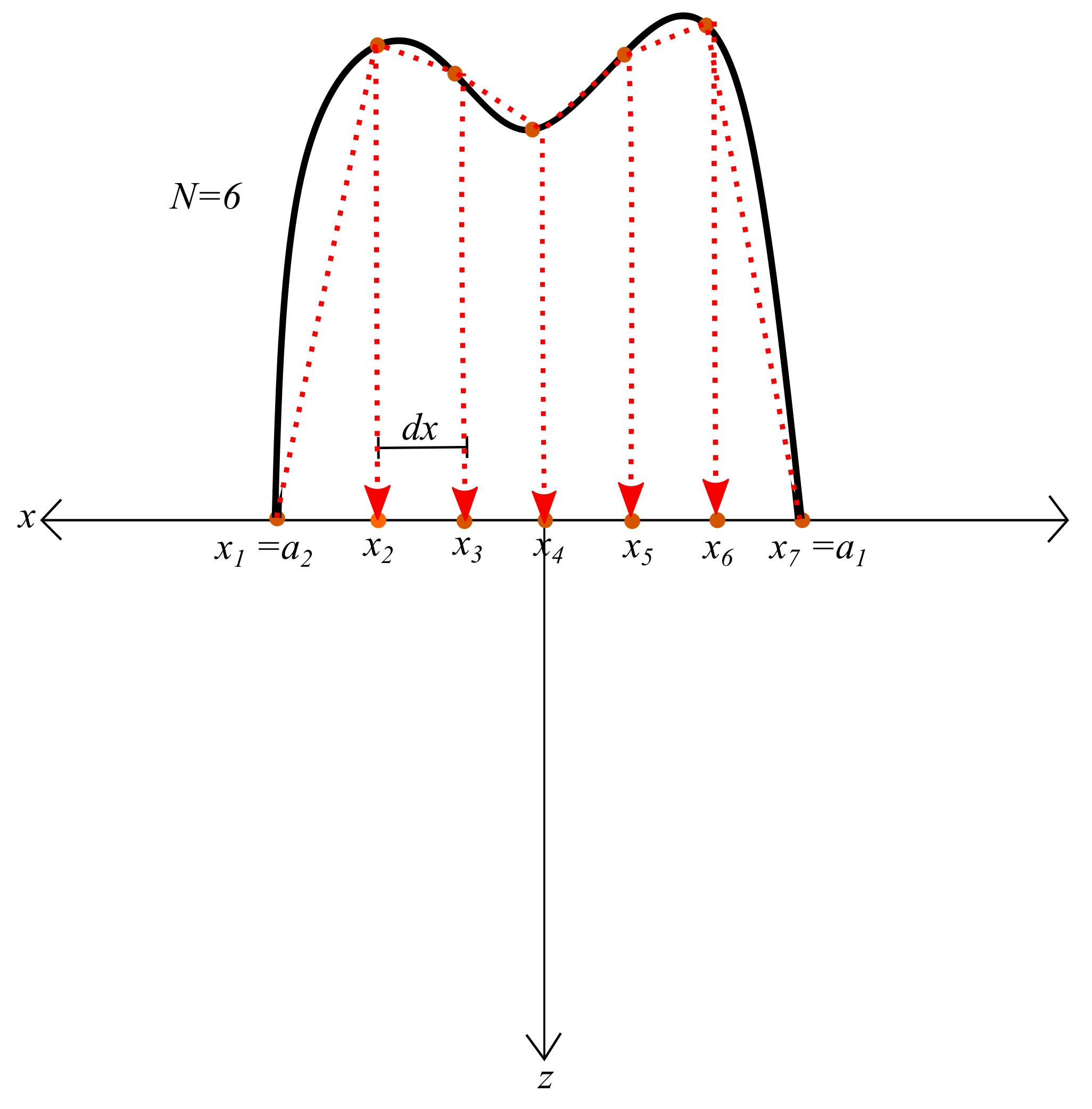
2.2. Approximate Solutions to Higher-Order Problems Via Superposition

The analytical solutions which provide the plane strain stress and strain fields for low-order (constant and linear) monomial traction boundary conditions in the Appendix A.1 and Appendix A.2 can be applied to construct approximate analytical solutions to general boundary value problems. The linearity of the governing partial differential equations assures that the superposition of solutions under varying boundary conditions provides a solution for more complex boundary data. The uniqueness of the solutions then assures that a determined series of solutions which converges to a given expression on the boundary converges to the solution of the corresponding boundary value problem within the problem domain (see [16,17]). The plane strain assumption makes it so this can be achieved through simple linear interpolation of arbitrary $p\left(x^{\prime }\right),q\left(x^{\prime }\right)$. This is shown by analytically approximating functions of the form

$$\begin{array}{c}\hfill \frac{{\partial }^{j+k}A}{\partial x^j\partial z^k}\equiv \underset{b\to \infty }{lim}\frac{{\partial }^{j+k}}{\partial x^j\partial z^k}{\int }_{-b}^b{\int }_{a_2}^{a_1}\frac{f\left(x^{\prime }\right)}{r}d{x}^{\prime }d{y}^{\prime },\end{array}$$

(21)

where $f\left(x^{\prime }\right)$ is an arbitrary, bounded, continuous ($C^0$) function representing p or q.

A Simple Algorithm

Discretize the region $a_2\le x^{\prime }\le a_1$ into N uniform subregions of width $dx$ as shown in Figure 3; the $N+1$ nodal interpolation points are then $x_i=a_2+(i-1)dx$, where $dx\equiv \frac{a_1-a_2}{N}$. The necessary derivatives of Equation (21) can be analytically approximated as a sum of N linear combinations of solutions of those of Equation (5) which correspond to the linear interpolations over the $x_i$. For example, assume the derivative $\frac{\partial A}{\partial z}$ is required, as in Equations (8)–(10) under arbitrary p. The potentials over the $i^{th}$ subregion $x_i\le x^{\prime }\le x_{i+1}$ corresponding to boundary traction of order m can then be written as $\frac{\partial A_i^m}{\partial z}$. The required potential can then be written as

$$\begin{array}{c}\hfill \frac{\partial A}{\partial z}\approx \sum _{i=1}^N\left(c_i^0\frac{\partial A_i^0}{\partial z}+c_i^1\frac{\partial A_i^1}{\partial z}\right).\end{array}$$

(22)

The relevant interpolation constants $c_i^m$ can be written as

$$\begin{array}{cc}\hfill & c_i^0=\frac{x_{i+1}p\left(x_i\right)+x_{i}p\left(x_{i+1}\right)}{dx}\hfill \end{array}$$

(23)

$$\begin{array}{cc}\hfill & c_i^1=\frac{p\left(x_{i+1}\right)+p\left(x_i\right)}{dx}\hfill \end{array}$$

(24)

This procedure is valid for all partial derivatives of the required potential functions, and also for arbitrary $q\left(x^{\prime }\right)$. It provides a simple but general means of approximating solutions to arbitrary boundary value problems via the linear combination and superposition of the few and simple expressions in the Appendix A.1 and Appendix A.2.

The simplicity of the linear interpolation scheme also allows for ease in error estimation. For example, let $e_p\left(x\right)$ be the error function between a normal traction distribution p and its linear interpolation as shown in Figure 3; it is known (e.g., [24]) that a sharp error bound can be given by

$$\begin{array}{c}\hfill max\left(e_p\left(x\right)\right)\le \frac{d{x}^2}{8}max\left|p^{″}\left(x\right)\right|.\end{array}$$

(25)

The uniqueness of the elastic field guarantees that the internal conditions converge alongside the conditions on the boundary.

The present approximation approach can be categorized as a numerical method as an instance of the Analytical Element Method (AEM) in elasticity. This method was originally developed by Strack [25,26] for the analysis of groundwater flow problems. In essence, AEM is equivalent to the Boundary Element Method (BEM), except the boundary integrals, dependent on the boundary conditions, are evaluated analytically. The closed-form solutions in the Appendix A.1 and Appendix A.2 can therefore be considered analytic elements for plane strain elastic contact problems.

3. Results

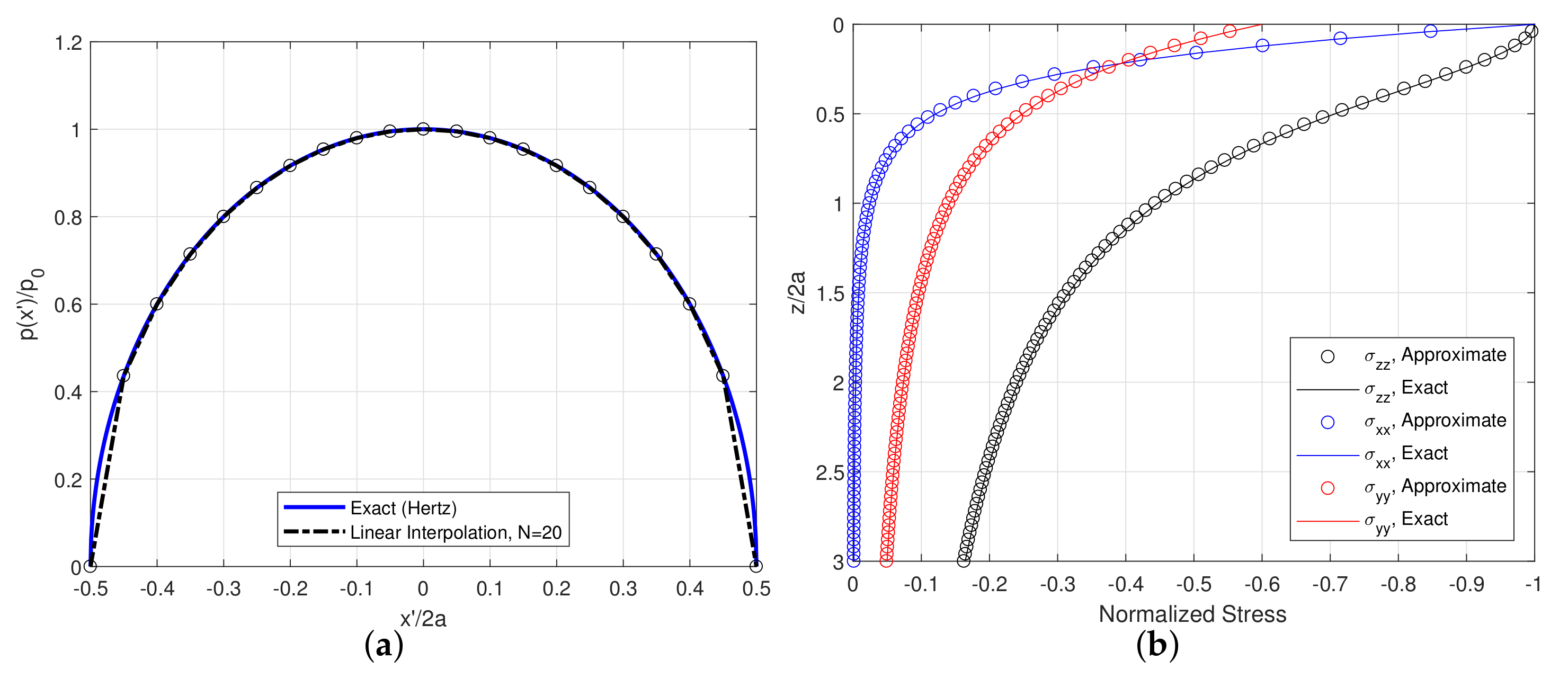
3.1. Verification Problem: Elastic Contact of Parallel Cylinders

The plane strain condition serves as an approximation of the problem of two long parallel elastic cylinders in contact. The contact for an arbitrary cross-section is also equivalent to the limit of a classic Hertzian contact [27] as the out-of-plane dimension becomes large. Similarly, the stress and strain fields can be considered as limit of the three-dimensional solutions given by Kunert [28] for Hertzian contact traction over a rectangular area. The simple algorithm presented in the last section can be verified in comparison to exact solutions for this classical problem.

Assuming a frictionless contact (i.e., $q\left(x^{\prime }\right)=0$), the contact traction field for an area of width $2a$, centered at the origin, is given by

$$\begin{array}{c}\hfill p\left(x^{\prime }\right)=p_0{\left(1-\frac{x^{\prime }{}^2}{a^2}\right)}^{1/2}.\end{array}$$

(26)

Equation (26) is shown in Figure 4a alongside its linear intepolation. Closed-form solutions for the internal stress fields beneath the center of the contact area are given in [29]. Figure 4b compares these internal stress fields with those approximated by the present method for $N=20$ discretized subregions.

The global error bound given by Equation (25) can not be calculated due to the fact that the slope of the tangent line of Equation (26) is infinite at the edge of the contact area; however, the stress fields still show strong convergence to the exact analytical solutions. Figure 5 shows that the the maximum error in the stress approximations of Figure 4 converge to zero with increasing N. The rate of convergence of the stress fields given by the present method is facilitated by the two-dimensional nature of plane strain problems. It is noted that simple Matlab code converges quickly for small N, and is noticeably faster than similar code employing bilinear interpolation for the fully three-dimensional contact problem (see [16,17]).

3.2. Applications to Shallow Foundation Analysis

The classical Boussinesq–Cerruti half-space problem has historically been applied to the analysis of soil–structure interaction, in particular the settlement and stress states in foundation systems [8,9,16,17,30]. The plane strain problem has been used as an approximation of strip foundations, wherein the aspect ratio of the footing is often large enough to neglect the length dimension. However, the contact and penetration behavior of granular soils is highly complex, and the observed contact traction and displacement fields generally vary non-linearly with a large range of multi-scale material and loading variables. There are therefore a large range of possibilities when selecting boundary conditions for this type of analysis; the generality of the calculation approach outlined here allows for the calculation and comparison of results for evolving contact traction fields from a wide array of sources. Two examples are chosen to highlight this application. The first involves an evolving normal contact traction field obtained analytically through an elastoplastic analysis [31]. This is used to investigate the strain response due to an increasingly loaded foundation. The second example applies traction fields which have been measured experimentally by Bauer et al. [32], acting in both the normal and tangential directions. These empirical traction fields are used to investigate the static stress behavior beneath a loaded strip foundation.

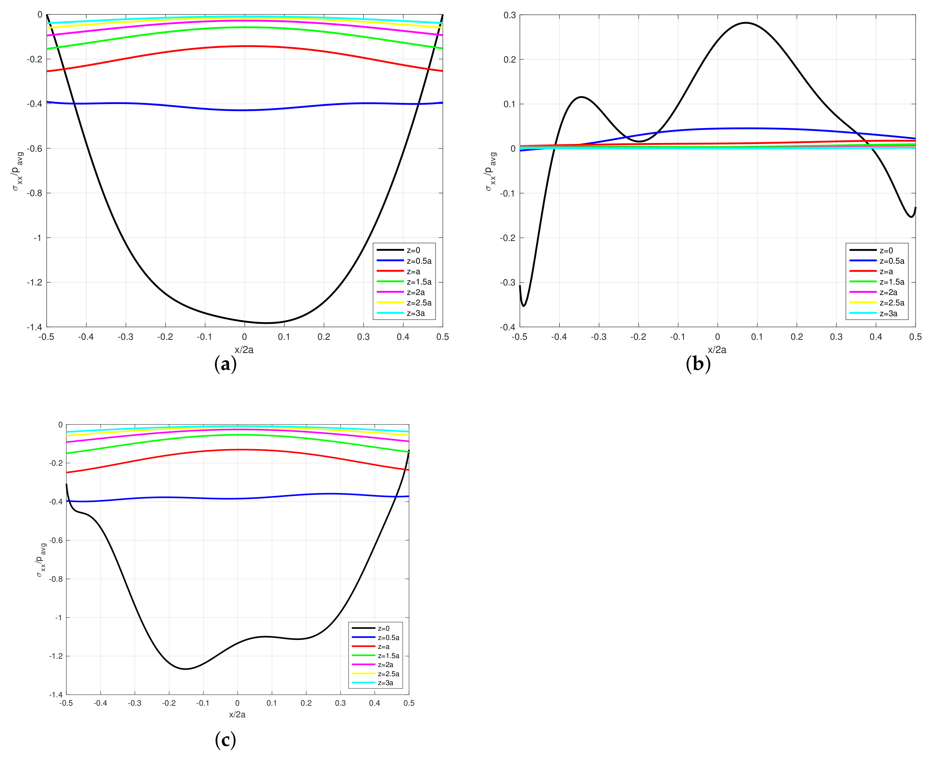
3.2.1. Example 1: Foundation Contact as an Elastoplastic Rigid Punch Problem

A loaded shallow foundation system is naturally modelled as a rigid punch problem, due to the fact that the footing is often relatively rigid in comparison to the underlying granular soil body. This type of problem is initially formulated using a mixed boundary condition [33,34,35], with displacements prescribed inside the contact region, and zero traction conditions applied outside on the surface of the half-space. Once the resulting surface traction fields are obtained corresponding to the prescribed displacements, equivalent solutions can be obtained by prescribing purely Neumann (traction) boundary conditions.

Boussinesq obtained the first solution [6,35] for a flat punch and showed that for purely elastic conditions, uniform surface displacement leads to singularities (infinite values) in the normal traction field at the edge of contact for any magnitude of indentation. Thus, any real elastic material will yield locally when indented any amount by a flat rigid punch. Schultze [36] initially combined Boussinesq’s result for elastic plane strain contact with the classical geotechnical theory of bearing capacity [37]; this led to a contact traction distribution which mimicked Boussinesq’s in a central elastic region but varied linearly to zero in an external plastic region. The contact traction therefore evolves with increasing load magnitude. Balakrishna [38] later extended this elastoplastic analysis to the three-dimensional case of an axisymmetric circular punch. Abdullah [31] later augmented Schultze’s results so that the traction in the plastic region varies quadratically. This was shown to agree better with numerical results; it also coincides more accurately with Terzaghi’s initial result for the traction at ultimate bearing capacity [37]. For these reasons, Abdullah’s traction field will be employed in the present example. Evolution of the contact traction from a purely elastic state to a quadratic plastic state at ultimate bearing capacity is shown in Figure 6 for a surface footing on a dry, dense sand.

The evolving traction fields shown in Figure 6 suggest a nonlinear displacement response of the foundation with increasing load, and hence a nonlinear elastic stiffness path. Recall from Section 2.1.2 that the displacement fields are not uniquely defined for the boundary conditions at infinity. However, the strain fields are well-defined, and the surface displacements can be approximated (at least qualitatively) by Equation (20), integrating a know strain field through the depth.

Figure 7a–c depicts the distributions of vertical strain ${ϵ}_{zz}$ with depth beneath three points of the loaded surface region. ${ϵ}_{zz}$ can be calculated from the stress components (Equations (8)–(11)) using Hooke’s law. The strain values are dependent on the Lame’s parameters $\lambda ,\mu$; these are chosen so that that corresponding Young’s modulus is $E=98,000$ kPa, and the Poisson’s ratio $\nu =0.4$. The peak strain location tends to decrease with increasing load at the center ($x=0$), while it increases at the midpoint from the edge ($x=0.5a$) and at the edge location ($x=a$). Furthermore, there exists a small region of elastic vertical tension beneath the edge of the load. This agrees with the three-dimensional elastic calculations of [16], and can be viewed as a necessary outcome of Hooke’s law and the zero-stress boundary conditions at this point. This phenomenon is therefore an outcome of the continuum-based approximation and must be considered non-physical if dealing with a granular soil.

Figure 7d shows approximate displacement points obtained by the numerical integration of the strain curves of Figure 7a–c. This provides a qualitative understanding of the evolution of stiffness across the width of the loaded footing predicted by the present elastoplastic model. This corresponds predictably with the evolution of contact traction shown in Figure 6. The bulk of the contact traction converges towards the center of the footing with increasing load, which corresponds to a softening of the stiffness curve at $x=0$. The contact stiffens at the footing’s edge ($x=a$) as the load becomes less concentrated in the neighborhood of this point, while the stiffness path halfway between the center and edge remains more or less linear. Importantly, non-uniform settlement develops, from which the vertical soil–foundation stiffness may affect bending moment distributions across the width of a strip footing even when relative length $b/a>10$.

The strain curves and displacements of Figure 7 are compared with a simplified Schmertmann strain influence analysis [10,11], in particular the type outlined in [39] for plane strain problems. For a critical analysis of Schmertmann’s method and variations, see [40]. This method estimates the settlement as:

$$\begin{array}{c}\hfill w_{Schmt}=p\sum _{i=1}^n{\left(\frac{I_z}{E}\Delta z\right)}_i,\end{array}$$

where $I_z$ in this case is given as a bilinear curve ranging linearly from 0.2 at $z/2a=0$ to 0.6 at $z/2a=0.5$, and then linearly to zero at $z/2a=4$; p is the average applied overpressure, and E the Young’s modulus, assumed constant in this case. The summation is taken over even intervals so that $\Delta z=8a/n$. Note the difference of the characteristics of Schmertmann’s influence factor and the strain curve under load $P_{ult}$ at $x=0$ in Figure 7a. The Schmertmann strain influence curve takes its peak at a deeper location beneath the load, and by assumption varies linearly to zero at $z/2a=4$; the calculated strain curves from elasticity have shallower peak locations and still take relatively large nonzero values at $z/2a=4$, as they go to zero in the limit at infinity. Note that Schmertmann’s method is included in Figure 7 only for the sake of comparison and to highlight these differences.

3.2.2. Example 2: Empirically Measured Contact Traction Fields from Real Granular Materials

A wide variety of experimental literature exists regarding contact traction fields beneath model or real footings founded on granular soils, e.g., [32,36,41,42,43,44]. In general, measurements of the frictional tangential contact traction fields are more difficult and rarely appear alongside the more easily-obtained normal distributions. Bauer et al. [32] and Muhs and Bub [43] provide measurements of both normal and tangential contact traction for various load magnitudes. Of these, Bauer’s experimental apparatus was specifically constructed to simulate plane strain conditions. For this reason, contact traction data from one of Bauer’s experimental cases is selected for an example study of the elastostatic stress equilibrium state beneath a strip footing.

The normal and tangential traction fields from the case selected from Bauer’s data are shown in Figure 8. It is assumed that both traction components take zero values at the footing’s edge; this is physically justified since the edge normal resistance of a surface footing must be zero, while the tangential value is bounded by the normal under a finite coefficient of friction. The assumption of zero edge values also allows for the removal of a jump discontinuity in the boundary conditions which is known to lead to singularities in the resulting stress tensor [8]. The distributions in Figure 8 are each the result of a curve fit of the resulting eight data points with a polynomial of the form

$$\begin{array}{c}\hfill f\left(x^{\prime }\right)=\sum _{n=0}^7{\alpha }_n{x}^{\prime }{}^n\end{array}$$

(27)

The curve-fit coefficients are listed in

Table 1. Curve-fit polynomial coefficients for Equation (27) which generate the traction distributions in Figure 8.

	${\mathit{\alpha }}_0$	${\mathit{\alpha }}_1$	${\mathit{\alpha }}_2$	${\mathit{\alpha }}_3$	${\mathit{\alpha }}_4$	${\mathit{\alpha }}_5$	${\mathit{\alpha }}_6$	${\mathit{\alpha }}_7$
$p\left(x^{\prime }\right)$	1.3756	0.2337	−1.5549	−4.8744	−29.4222	36.5699	54.5259	−83.2448
$q\left(x^{\prime }\right)$	−0.0695	0.7026	2.8446	−12.6194	−27.3084	106.2138	68.1680	−267.9106

. The traction fields are normalized by the average normal pressure $p_{avg}$, obtained by the integration of the polynomial resulting from the curve-fit of the normal traction data. The lack of perfect symmetry in the traction data may stem from a combination of eccentricity in the load and inhomogeneity in the soil samples in [32].

Figure 9 shows the vertical stress (${\sigma }_{zz}$) distributions at various depths beneath the loaded boundary region. Figure 9a,b show the components of ${\sigma }_{zz}$ due to the normal and tangential components of the boundary conditions, respectively. Note that the lack of symmetry in the boundary conditions in rapidly smoothed out with depth within the elastic media; this can be viewed as a necessary outcome of Saint Venant’s principle [45]. It is clear that in this case ${\sigma }_{zz}$ is dominated by the normal traction component, as one might expect. The total combined values of ${\sigma }_{zz}$ differ negligibly from those under the influence of $p\left(x^{\prime }\right)$ alone, as shown in Figure 9c. This is in contrast to the results of [17,18], where the assumed radial tangential contact traction was large enough to have a considerable qualitative and quantitative effects on the internal vertical stress distributions.

Figure 10 and Figure 11 show the same distributions for the horizontal and shear stresses ${\sigma }_{xx}$ and ${\sigma }_{xz}$, respectively. In both the cases the stress components are more noticeably influenced by the presence of the surface frictional tangential traction q. This component of contact traction will therefore influence the overall behavior of the principle stress fields in the present case. This suggests that the modes of distribution of the shearing traction component may be non-negligible when assessing the equilibrium states of shallow foundation systems.

The preceding stress tensor calculations can be combined to form the following two quantities: the hydrostatic pressure

$$\begin{array}{c}\hfill P=\frac{1}{3}({\sigma }_{xx}+{\sigma }_{yy}+{\sigma }_{zz}),\end{array}$$

(28)

and the von Mises stress

$$\begin{array}{cc}\hfill & {\sigma }_v=\sqrt{3J_2},\hfill \\ \hfill & J_2=\frac{1}{6}\left({({\sigma }_{xx}-{\sigma }_{yy})}^2+{({\sigma }_{yy}-{\sigma }_{zz})}^2+{({\sigma }_{zz}-{\sigma }_{xx})}^2\right)+{\sigma }_{xz}^2.\hfill \end{array}$$

(29)

Recall that the presence of ${\sigma }_{yy}$ in quantities (28) and (29) implies a dependence on the Poisson ratio $\nu$. The hydrostatic pressure and von Mises stress are plotted in Figure 12 for a value of $\nu =0.4$.

Finally, Bauer’s paper appears unique in that it provides load–settlement data alongside the contact traction measurements. This allows for a calibration of the strain-influence method of settlement estimation used in Example 1 via Equation (20). For reference, the footing in Bauer’s experiment had total width of 0.305 m; the traction values for our example shown in Figure 8 have been normalized by a factor of $p_{avg}=119.09$ kPa, calculated by integrating the polynomial fit of Bauer’s data using Equation (27). The soil sample was a crushed quartz sand with known density (15.7 kN/m${}^3$) and internal friction angle (45 degrees). Bauer reported a settlement of approximately 1 cm for this loading case (test 1, load 2).

Figure 13 shows the strain under the center of the footing estimated by the present method with a fixed Poisson ratio of 0.4. The strain values are multiplied by the Young’s modulus, which is unknown in this case. Note that the presence of the shearing traction has negligible effect on the normal strain (and thus the soil–structure stiffness): this is in good agreement with the results of [17,18]. Integrating the strain curves from the combined loading yields a value of $wE=48.798$ kPa-m; thus, the model requires a Young’s modulus of around 5000 kPa to match the measured settlement value.

4. Discussion and Conclusions

Constant and linear analytic elements have been developed for the Neumann boundary value problem of a homogeneous and isotropic elastic half-plane under plane strain conditions. These are derived as the spatial limit of similar three-dimensional solutions over rectangular areas. A simple algorithm for superposition of solutions corresponding to linear interpolants of boundary conditions provides a convenient method for the analysis of general contact problems prescribing arbitrary distributions of normal and tangential surface traction.

Examples related to soil–structure interaction were selected to highlight the application of the proposed method. The elastoplastic normal tractions from Example 1 were selected in part to highlight the fact that contact is almost always a nonlinear phenomenon; evolving boundary conditions will introduce nonlinearity to an otherwise linear problem. It is worth noting that some error in this case is likely, due to the application of boundary conditions derived in part from plasticity in a purely elastic domain. However, based on Figure 7, it is clear that some of the expected nonlinearity in the load–displacement behavior is captured by the present method, while absent from the Schmertmann example. Interestingly, despite the discussed physical differences between the strain curves in the two methods, the present method yields settlement estimates at the center of the load which are strikingly close to the Schmertmann values. The similarity in the estimated settlements suggests that analysis can be improved by employing well-derived or measured boundary conditions, even when using a simple linear elastic constitutive model.

The selection of the empirically-measured normal and tangential tractions in Example 2 were motivated by recent work that suggests that the presence of the tangential contact traction fields may have a non-negligible effect on the analysis [17,18]. In particular, the tangential traction field should be included in a contact problem with friction if accuracy in the local stress tensor is desired. The data from [32] was chosen because it is one of few places where both normal and tangential fields were recorded and published for a problem approximating plane strain conditions. Far more research is needed before the normal and tangential contact traction fields can be accurately predicted a priori for a given soil–structure system, as they are dependent on the load magnitude and geometry and a plethora of uncertain multiscale properties of the granular material. The uncertainty and heterogeneity related to the evolution of contact traction fields generated between structural footings and underlying soils may make the present method attractive to geotechnical engineers and analysts wishing to assess the elastic settlement and equilibrium states of shallow foundation systems under varying assumptions.

One major limitation of the application of this model to soil–structure interaction is the problem of scaling: there is a known scale-dependency of soil–foundation vertical stiffness. The present examples have normalized the boundary conditions by footing size and load magnitude, while some of the real scale-dependency stems from the interactions with a complex granular body. Further work may try to calibrate the model to site-scale settlement measurements (e.g., [46]), but the true utility of this model can only be assessed if load–settlement data is presented alongside the measured contact traction fields. The argument here is that some of the nonlinearity from the scale and load dependence can be captured by accurate boundary conditions.

There is further uncertainty introduced in the present model when assessing the material constants. Clearly, there are natural limitations when using any continuum method to describe the mechanics of granular materials. The uncertainty increases when using the simplest possible constitutive model with two elastic constants. The effects of varying the Poisson ratio in the present model is non-negligible when exact results are required, but small when compared with uncertainty in the boundary conditions, influence depth, and Young’s modulus; thus, the value of 0.4 was deemed reasonable for use throughout this entire paper.

The value of Young’s modulus used in Example 1 (i.e., 98,000 kPa) was deemed a decent estimate for a dense homogeneous sand by assessing values listed in a classic geotechnical reference [47]. However, the value required to match the settlement measurement of Bauer in Example 2 was an order of magnitude smaller (approximately 5000 kPa). This value also seems reasonable when when compared to those used by Schmertmann when estimating the modulus from cone penetration test data [10]. Even a “homogeneous” soil will have variations in the modulus from this estimate with depth. This further exacerbates the issue of sensitivity to strain influence depth and the problem with scaling. The Schmertmann method is designed to account for this material heterogeneity, while the present solutions are for a truly homogeneous material sans body forces. Applying the strain predictions from this model over layers of varying elastic moduli has not been tested or verified against any known data. One approximate workaround is to do the analysis based on in-situ measurements and then take an average to assess the effective Young’s modulus for the homogeneous problem. Ultimately, the “elastic modulus” is not a real attribute of a granular body, but instead a parameter of idealized models which may take different values in different contexts. The value determined from triaxial test data may not be the same as the value correlated from a cone penetration test (or that which is required to match a measured settlement when analyzing the soil–structure contact problem). The analyst must be ever-cognizant of this fact.

The solutions presented here are analytic solutions to a type of boundary value problem that has historically been applied to geotechnical problems, but the assumptions in the model are vast over-simplifications of any real soil–structure interaction problem. The purpose of this work was to provide incremental progress by generalizing the types of boundary conditions that can easily be assessed. However, the solutions and method are applicable to more general non-Hertzian contacts and may also be of use to practitioners in the field of tribology. They can be applied to assess the internal stress and strain field for any contact situation in which the plane strain assumption is valid and when surface traction fields can be measured or deduced a priori.

References

1. Flamant, A. Sur la repartition des pressions dans un solide rectangulaire charge transversalement. Compt. Rendus 1892, 114, 1465. [Google Scholar]
2. Johnson, K. Contact Mechanics; Cambridge University Press: Cambridge, UK, 1985. [Google Scholar]
3. Hemsley, J. Elastic Analysis of Raft Foundations; Thomas Telford Publishing: London, UK, 1998. [Google Scholar] [CrossRef]
4. Muskhelishvili, N. Some Basic Problems of the Mathematical Theory of Elasticity; P. Noordhoff: Groningen, The Netherlands, 1963. [Google Scholar]
5. England, A. Complex Variable Methods in Elasticity; Dover Publications: Mineola, NY, USA, 1971. [Google Scholar]
6. Boussinesq, J. Application Des Potentials a l’etude de l’equilibre et du Mouvement des Solides Elastiques; Gauthier-Villars: Paris, France, 1885. [Google Scholar]
7. Boussinesq, J. Essai theorique sur l’equilibre d’elasticite des massifs pulverulents compare a celui de massifs solides et sur la poussee des terres sans cohesion. In Mémoires Couronnés et Mémoires des Savants Étrangers; Forgotten Books: London, UK, 1876. [Google Scholar]
8. Love, A.E.H. The stress produced in a semi-infinite solid by pressure on part of the boundary. Philos. Trans. R. Soc. Lond. Ser. Contain. Pap. Math. Phys. Character 1929, 228, 377–420. [Google Scholar]
9. Newmark, N.M. Simplified Computation of Vertical Pressures in Elastic Foundations; Report, Engineering Experiment Station; University of Illinois at Urbana-Champaign: Champaign, IL, USA, 1935. [Google Scholar]
10. Schmertmann, J. Static cone to compute static settlement over sand. J. Mech. Found. Div. ASCE 1970, 96, 1011–1043. [Google Scholar] [CrossRef]
11. Schmertmann, J.; Hartman, J.; Brown, P. Improved strain influence factor diagrams. J. Geotech. Geoenviron. Eng. 1978, 104, 1131–1135. [Google Scholar] [CrossRef]
12. Shahriar, M.A.; Sivakugan, N.D.B. Strain influence factors for footings on an elastic medium. In Proceedings of the ANZ 2012 Conference Proceedings, Melbourne, Australia, 9–13 August 2012. [Google Scholar]
13. Pantelidis, L. Elastic Settlement Analysis for Various Footing Cases Based on Strain Influence Areas. Geotech. Geol. Eng. 2020, 38, 4201–4225. [Google Scholar] [CrossRef]
14. Pantelidis, L. Strain Influence Factor Charts for Settlement Evaluation of Spread Foundations based on the Stress–Strain Method. Appl. Sci. 2020, 10, 3822. [Google Scholar] [CrossRef]
15. Pantelidis, L.; Gravanis, E. Elastic Settlement Analysis of Rigid Rectangular Footings on Sands and Clays. Geosciences 2020, 10, 491. [Google Scholar] [CrossRef]
16. Taylor, A.G.; Chung, J.H. Application of low-order potential solutions to higher order vertical traction boundary problems in an elastic half-space. R. Soc. Open Sci. 2018, 5, 180203. [Google Scholar] [CrossRef]
17. Taylor, A.G.; Chung, J.H. Analysis of tangential contact boundary value problems using potential functions. R. Soc. Open Sci. 2019, 6, 182106. [Google Scholar] [CrossRef]
18. Taylor, A.G.; Chung, J.H. Explanation and Application of the Evolving Contact Traction Fields in Shallow Foundation Systems. Geotechnics 2022, 2, 4. [Google Scholar] [CrossRef]
19. Marmo, F.; Rosati, L. A general approach to the solution of Boussinesq’s problem for polynomial pressures acting over polygonal domains. J. Elast. 2015, 122, 75–112. [Google Scholar] [CrossRef]
20. Marmo, F.; Sessa, S.; Rosati, L. Analytical solutions of the Cerruti problem under linearly distributed horizontal loads over polygonal domains. J. Elast. 2016, 124, 27–56. [Google Scholar] [CrossRef]
21. Love, A.E.H. A Treatise on the Mathematical Theory of Elasticity; Dover Publications: New York, NY, USA, 1944. [Google Scholar]
22. Cerruti, V. Ricerche intorno all’equilibrio de’corpi elastici isotropi. R. Accad. Dei Lincei 1882, 13, 81–123. [Google Scholar]
23. Abdeyev, B.; Brim, T.; Muslimanova, G. Contradictions in the plane contact problem of the theory of elasticity on the compression of cylinders in contact with parallel generators. PNRPU Mech. Bulletic 2021, 6–11. [Google Scholar] [CrossRef]
24. Yano, M.; Penn, J.; Konidaris, G.; Patera, A. Maths, Numerics, and Programming (for Mechanical Engineers); MIT OpenCourseWare: Cambridge, MA, USA, 2013. [Google Scholar]
25. Strack, O. The Analytic Element Method for regional groundwater modelling. In Proceedings of the Conference of the National Water Well Association Solving Groundwater Problems with Models, Dublin, OH, USA, 10–12 February 1987. [Google Scholar]
26. Strack, O. Groundwater Mechanics; Prentice Hall: Englewood Cliffs, NJ, USA, 1989. [Google Scholar]
27. Hertz, H. On the Contact of Rigid Elastic Solids and on Hardness; Chapter 6: Assorted papers by H. Hertz; MacMillan: New York, NY, USA, 1882. [Google Scholar]
28. Kunert, V.K. Spannungsverteilung im Halbraum bei elliptischer Flächenpressungsverteilung über einer rechteckigen Druckfläche. Forsch. Auf Dem Geb. Des Ingenieurwesens A 1961, 27, 165–174. [Google Scholar] [CrossRef]
29. Williams, J.; Dwyer-Joyce, R. Modern Tribology Handbook, Chapter 3: Contact Between Solid Surfaces; CRC Press: Boca Raton, FL, USA, 2001. [Google Scholar]
30. Davis, R.O.; Selvadurai, A.P.S. Elasticity and Geomechanics; Cambridge University Press: Cambridge, UK, 1996. [Google Scholar]
31. Abdullah, W. New elastoplastic method for calculating the contact pressure distribution under rigid foundations. Jordan J. Civ. Eng. 2008, 2, 71–89. [Google Scholar]
32. Bauer, G.; Shields, D.; Scott, J.; Nwabuokei, S. Normal and shear stress measurements on a strip footing. Can. Geotech. J. 1979, 16, 177–189. [Google Scholar] [CrossRef]
33. Fabrikant, V. Flat punch of arbitrary shape on an elastic half-space. Int. J. Engng. Sci. 1986, 24, 1731–1740. [Google Scholar] [CrossRef]
34. Harding, J.; Sneddon, I. The elastic stresses produced by the indentation of the plane surface of a semi-infinite elastic solid by a rigid punch. In Mathematical Proceedings of the Cambridge Philosophical Society; Cambridge University Press: Cambridge, UK, 1945; Volume 41, pp. 16–26. [Google Scholar]
35. Sneddon, I. Boussinesq’s problem of a flat-ended cylinder. Math. Proc. Camb. Phil Soc. 1946, 42, 29–39. [Google Scholar] [CrossRef]
36. Schultze, E. Distribution of stress beneath a rigid foundation. In Proceedings of the 5th International Conference on Soil Mechanics and Foundation Engineering, Paris, Frace, 17–22 July 1961; pp. 807–813. [Google Scholar]
37. Terzaghi, K. Theoretical Soil Mechanics; John Wiley and Sons, Inc: New York, NY, USA, 1943. [Google Scholar]
38. Balakrishna, C.; Murthy, B.; Nagaraj, T. Stress distribution beneath rigid circular foundations on sands. Int. J. Numer. Anal. Methods Geomech. 1992, 16, 65–72. [Google Scholar] [CrossRef]
39. Terzaghi, K.; Ralph, B.P.; Mesri, G. Soil Mechanics in Engineering Practice; Wiley: London, UK, 1996. [Google Scholar]
40. Pantelidis, L. A Critical Review of Schmertmann’s Strain Influence Factor Method for Immediate Settlement Analysis. Geotech. Geol. Eng. 2020, 38, 1–18. [Google Scholar] [CrossRef]
41. Ho, M.; Lopes, R. Contact pressure of a rigid circular foundation. J. Soil Mech. Found. Div. Proc. Am. Soc. Civ. Eng. 1969, 93, 791–802. [Google Scholar] [CrossRef]
42. Lazebnik, G.E.; Smirnov, A.A. Measurement of stresses under a rigid foundation block in the field. Soil Mech. Found. Eng. 1964, 1, 71–78. [Google Scholar] [CrossRef]
43. Muhs, H.; Bub, H. On the measurement of friction in the base of flat footings founded in sand and first test results gained by a new gauge developed for the combined measurement of normal and tangential stresses. In Proceedings of the 6th International Conference of Soil mechanics and Foundation Engineering, Montreal, QC, Canada, 8–15 September 1965; Cambridge University Press: Cambridge, UK, 1965. [Google Scholar]
44. Murzenko, Y. Experimental results on the distribution of normal contact pressure on the base of a rigid foundation resting on sand. Soil Mech. Found. Eng. 1965, 2, 69–73. [Google Scholar] [CrossRef]
45. von Mises, R. On Saint Venant’s principle. Bull. AMS 1945, 51, 555–562. [Google Scholar] [CrossRef]
46. Briaud, J.L.; Gibbens, R. Behavior of Five Large Spread Footings in Sand. J. Geotech. Geoenvironmental Eng. 1999, 125, 787–796. [Google Scholar] [CrossRef]
47. Lambe, T.; Whitman, R. Soil Mechanics; John Wiley & Sons: New York, NY, USA, 2008. [Google Scholar]
Figure 1. (a) Geometry of a three-dimensional Cartesian elastic half-space, with a loaded rectangular region of width 2 a and length 2 b , centered at the origin. (b) Geometry of the plane-strain problem, which results from taking the limit of the three-dimensional problem as b .
Geotechnics 02 00032 g001
Figure 2. A demonstration that the magnitude of the three-dimensional potential A 00 (Equation (2)) grows without bound as the dimension b of the loaded rectangular region R becomes large. Thus Equations (17) and (18) are not well defined for constant surface traction.
Geotechnics 02 00032 g002
Figure 3. An example of the discretization of the loaded domain and the interpolation of a traction field using linear elements.
Geotechnics 02 00032 g003
Figure 4. (a) The plane strain Hertz contact pressure field given by Equation (26), along with a linear interpolation consisting of N = 20 discretized subregions. (b) Comparison of the exact internal stress fields given in [29] with those approximated using the superposition of 20 potentials corresponding to the linear interpolants. The out-of-plane stress σ y y is calculated for a Poisson’s ratio ν = 0.3 .
Geotechnics 02 00032 g004
Figure 5. Convergence with N of the maximum error for the stress fields shown in Figure 4.
Geotechnics 02 00032 g005
Figure 6. Example normal contact traction field distributions for an elastoplastic rigid punch foundation loaded on the surface of a dry, cohesionless sand (from Abdullah [31]). The traction field evolves inwards towards the bounding quadratic curve for a load P u l t , determined by the classical bearing capacity theory [37]. The traction fields are normalized by the ultimate average pressure p u l t = P u l t / 2 a .
Geotechnics 02 00032 g006
Figure 7. Vertical strain ϵ z z and approximate displacements beneath the evolving elastoplastic loading conditions of Figure 6. Elastic constants are taken as E = 98 , 000 kPa, ν = 0.4 . (a) ϵ z z at x = 0 ; (b) ϵ z z at x = 0.5 a ; (c) ϵ z z at x = a ; (d) Approximate displacements estimated by Equation (20) with applied force, normalized by bearing capacity P u l t .
Geotechnics 02 00032 g007
Figure 8. Example normal and shear contact traction fields from Bauer et al. [32]. Data points from test 1, load #2 of [32] curve-fit using 7th order polynomial functions to provide continuous expressions for boundary conditions.
Geotechnics 02 00032 g008
Figure 9. Vertical stress σ z z at various depths due to (a) normal component of boundary traction p ( x ) ; (b) tangential component of boundary traction q ( x ) ; (c) both p ( x ) and q ( x ) .
Geotechnics 02 00032 g009
Figure 10. Horizontal stress σ x x at various depths due to (a) normal component of boundary traction p ( x ) ; (b) tangential component of boundary traction q ( x ) ; (c) both p ( x ) and q ( x ) .
Geotechnics 02 00032 g010
Figure 11. Shearing stress σ x z at various depths due to (a) normal component of boundary traction p ( x ) ; (b) tangential component of boundary traction q ( x ) ; (c) both p ( x ) and q ( x ) .
Geotechnics 02 00032 g011
Figure 12. (a) The hydrostatic pressure P from Equation (28) under the combined normal and tangential traction boundary conditions shown in Figure 8 for Poisson ratio ν = 0.4 . (b) The von Mises stress σ v from Equation (29) under the same conditions.
Geotechnics 02 00032 g012
Figure 13. Calculated strains beneath the center of the examined load case from Bauer et al. [32] (Figure 8).
Geotechnics 02 00032 g013