Article

Fluid–Structure Interaction Modeling of Ascending Thoracic Aortic Aneurysms in SimVascular

1
Research and Development Unit for Mechanical and Industrial Engineering (UNIDEMI), Department of Mechanical and Industrial Engineering, NOVA School of Science and Technology, NOVA University Lisbon, 2829-516 Caparica, Portugal
2
Department of Cardiothoracic Surgery, Santa Marta Hospital, 1169-024 Lisboa, Portugal
3
Mines Saint-Etienne, University of Lyon, Inserm, Sainbiose U1059, F-42023 Saint-Etienne, France
*
Author to whom correspondence should be addressed.
Biomechanics 2022, 2(2), 189-204; https://doi.org/10.3390/biomechanics2020016
Submission received: 24 February 2022 / Revised: 25 April 2022 / Accepted: 28 April 2022 / Published: 1 May 2022
(This article belongs to the Section Tissue and Vascular Biomechanics)

Abstract

:
Ascending Thoracic Aortic Aneurysm (ATAA) is a permanent dilatation of the aorta which is usually related to tissue degeneration, hemodynamic conditions, lifestyle, environmental and genetic factors. As the mechanical conditions can become critical in a dilated aorta, a patient-specific computational model can be very useful to assist clinical decisions in the management of ATAAs. In this article, we model the biomechanical conditions of ATAA by performing Fluid–Structure Interaction (FSI) simulations in the SimVascular open-source software package. The patient-specific geometric model is reconstructed from Computed Tomography scan (CT). The numerical implementation takes into account patient-specific outlet conditions and a temporal flow variation at the model inlet. We performed a mesh convergence analysis on a new mesh reconstruction method in SimVascular and showed that it can significantly reduce the computational cost without impacting the accuracy.

1. Introduction

Aging, genetic, environmental and lifestyle factors, together with Bicuspid Aortic Valve (BAV), can lead to the formation of an Ascending Thoracic Aortic Aneurysm (ATAA) [1,2]. Guidelines from the European Society of Cardiology (ESC) define ATAA as a diameter increase of at least 50 % and recommend surgery if the maximal diameter exceeds 55 m m [3]. However, 60 % of patients who develop aortic dissections, which are the most catastrophic complication related to ATAA, had a diameter below the threshold of 55 m m [4,5]. Therefore, the guidelines supporting clinical decisions need to be completed with other stratification criteria based on both hemodynamics and biomechanics [6,7,8].
In recent decades, computational mechanics has been used to model the development and progression of aortic aneurysms, taking into account hemodynamics [9,10], wall mechanics [7,11,12] and mechanobiology [13,14]. More specifically, Computational Solid Mechanics (CSM) by the Finite Element Method (FEM) are used both at the macro [2,15] and micro [16,17] scale. Taghizadeh et al. [14] and Thunes et al. [18] studied, respectively, the effect of hypertensive and uniaxial loading conditions on idealized aortic models. Gültekin et al. [12] and Ban et al. [19] implemented a computational representation of extension–distension–torsion and biaxial experimental tests. Wang et al. [20] studied the effect of glycation on Aortic Dissection (AD) progression. Mousavi et al. [21] solved an inverse problem to characterize the patient-specific hyperelastic behaviour of the aortic wall. Moreover, Hackstein et al. [22] used Artificial Intelligence (AI) to identify new hemodynamics-based metrics that correlates with certain pathological states.
AI can help to reduce computational requirements in solving these complex problems. Its adaptability has become attractive: (1) to reduce the human effort in pre-processing, namely in the segmentation or analysis of medical imageology in the 3D geometric reconstruction of patient-specific aortic aneurysm structure [23,24,25]; (2) to improve the reporting efficiency of medical imaging exams [26]; (3) to provide an early-stage prediction of rupture risk and site [27,28]; (4) to evaluate the in vivo mechanical parameters of the aortic wall tissue [15,29,30]; (5) to act as a wall constitutive model [31]; or (6) to estimate the non-loaded configuration of ATAA [32]. Furthermore, it has been used to sometimes replace CSM [15,28,33].
Computational Fluid Dynamics (CFD) models are useful to hemodynamics changes induced by the growth of the aneurysm [10,17] or the presence of AD [34,35,36], such as flow patterns, blood pressure or Wall Shear Stress (WSS) distributions, and the risk of acute events [37,38,39,40]. Zhang et al. [34] and Long Ko et al. [35] studied the underlying mechanisms of AD by evaluating the effect of pulsatile flow conditions on patient-specific geometries. Mourato et al. [10] and Simão et al. [39] developed a numerical model of ATAA hemodynamics using patient-specific models. Capellini et al. [17] applied mesh morphing techniques and reduced-order models to study the effect of aneurysm growth on hemodynamics. Condemi et al. [38] combined CFD and Magnetic Resonance Imaging (MRI) to study the correlation of WSS and rupture risk. Pasta et al. [37] found correlations between WSS biomarkers from blood samples analyses.
Fluid–Structure Interaction (FSI) models simulate the interaction between the blood flow and the aortic wall, providing a more realistic and accurate numerical description. Yeh et al. [41] studied the biomechanical behaviour of ATAA under hypertensive conditions. Chen et al. [42] applied a FSI model to analyse the dynamics of the flap in AD. Mendez et al. [43] performed a comparative study between CSM, CFD and FSI approaches and reported that FSI models needed for variations in the diameter of the order of 10–15% over the cardiac cycle. Nonetheless, the use of FSI also represents a computational effort that may not be compatible with clinical applications [43,44,45].
Several computing platforms are available to perform FSI simulations [43,46,47,48]. Among them, SimVascular was developed as an open source software dedicated to cardiovascular simulations [49]. The software allows the reconstruction of the geometric model from DICOM images and the numerical analysis for both CFD and FSI using the Arbitrary Lagrangian–Eulerian (ALE) method.
In this work, we developed FSI models of ATAA using SimVascular. We developed an optimized method for mesh generation, enabling a significant gain in computational time.

2. Methods

2.1. Overview of Mathematical Models

2.1.1. Fluid Domain

The fluid domain is modeled by solving the Navier–Stokes and the continuity equations. It was simplified as incompressible, homogeneous, and with a Newtonian behaviour. These assumptions are widely accepted in hemorheology while studying blood flow in large vessels [31,39,50,51,52],
ρ f u t + ( ( u w ) · ) u · σ f u , p = 0 , in Ω f
· u = 0 , in Ω f
where t, ρ f , p, u , and w are the time, fluid density, pressure, velocity and the moving coordinate velocity, respectively. The term ( u w ) is specific to the ALE formulation and expresses the relative fluid velocity with respect to the grid velocity [53]. Furthermore, this equation utilizes the ALE time-derivative. The Cauchy stress ( σ f ) is defined such as σ f u , p = 2 μ D u p I , where I is the identity tensor, and D u = 1 2 u + T u .

2.1.2. Solid Domain

The aorta is modeled as an incompressible, anisotropic and hyperelastic material [54,55,56]. The Cauchy stress tensor may be written such as,
σ i j = 1 J F i k W F k j
where F is the deformation gradient tensor, W is the strain energy function and J is the Jacobian, which J = det ( F ) .

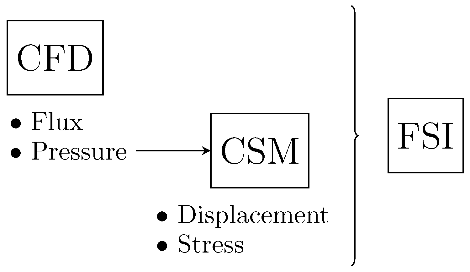
2.1.3. Fluid–Structure Interaction

The fluid and the solid domains are coupled through Equations (4) and (5) such as [57]
u = t v
σ f n f + σ s n s = 0
where u and v are the fluid velocity and the displacement fields, respectively. Furthermore, σ f is the Cauchy stress tensor and n f is the unit normal to the surface, both in the fluid domain and σ s , n s are the counterparts for the solid domain.

2.2. Hyperelastic Constitutive Model

A Neo–Hookean strain energy density was assumed, such as
W = μ s 2 I ¯ 1 3 + K s 2 ( J 1 ) 2
where μ s , K s are material properties, namely shear modulus and bulk modulus, respectively, for small deformations and I 1 is the first invariant. Accordingly, the Cauchy stress tensor can be described as follows,
σ i j = μ s J 5 / 3 B i j 1 3 B k k δ i j + K s ( J 1 ) δ i j
where B is the left Cauchy–Green deformation tensor.
All material constants are reported in Table 1 [57].

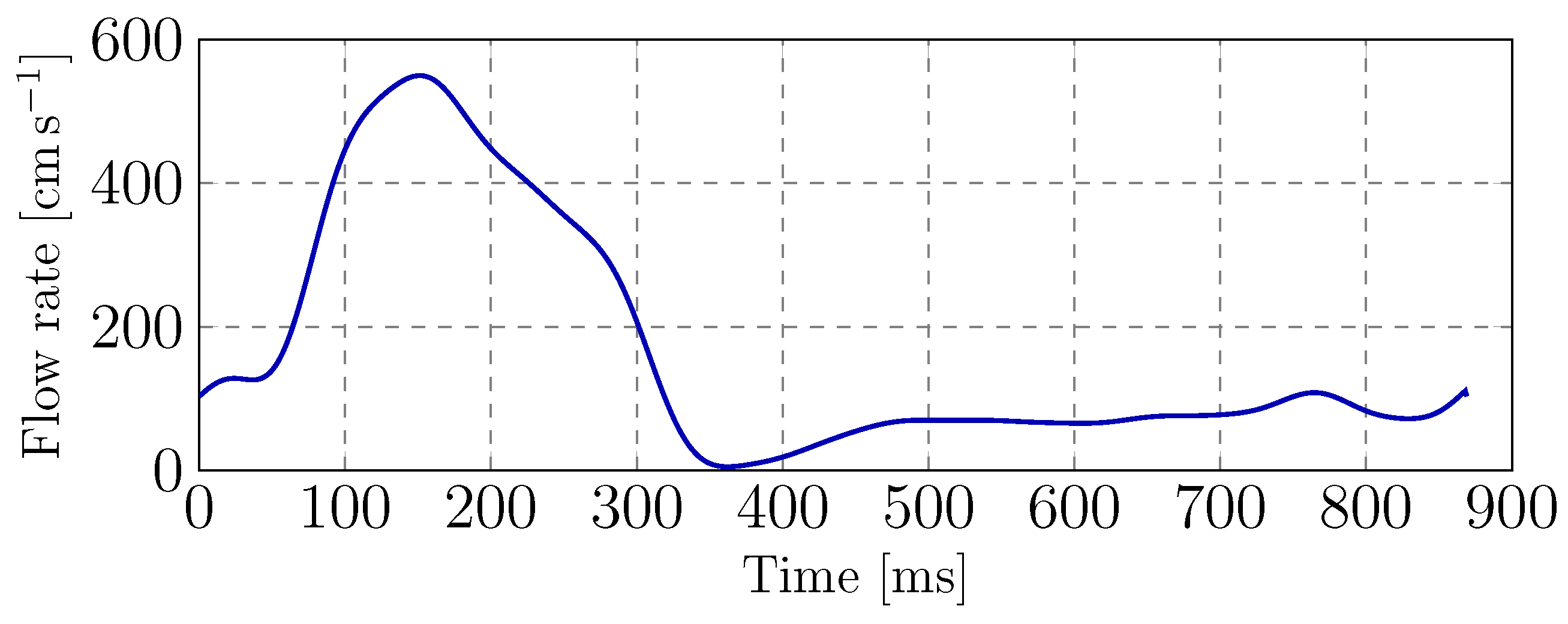
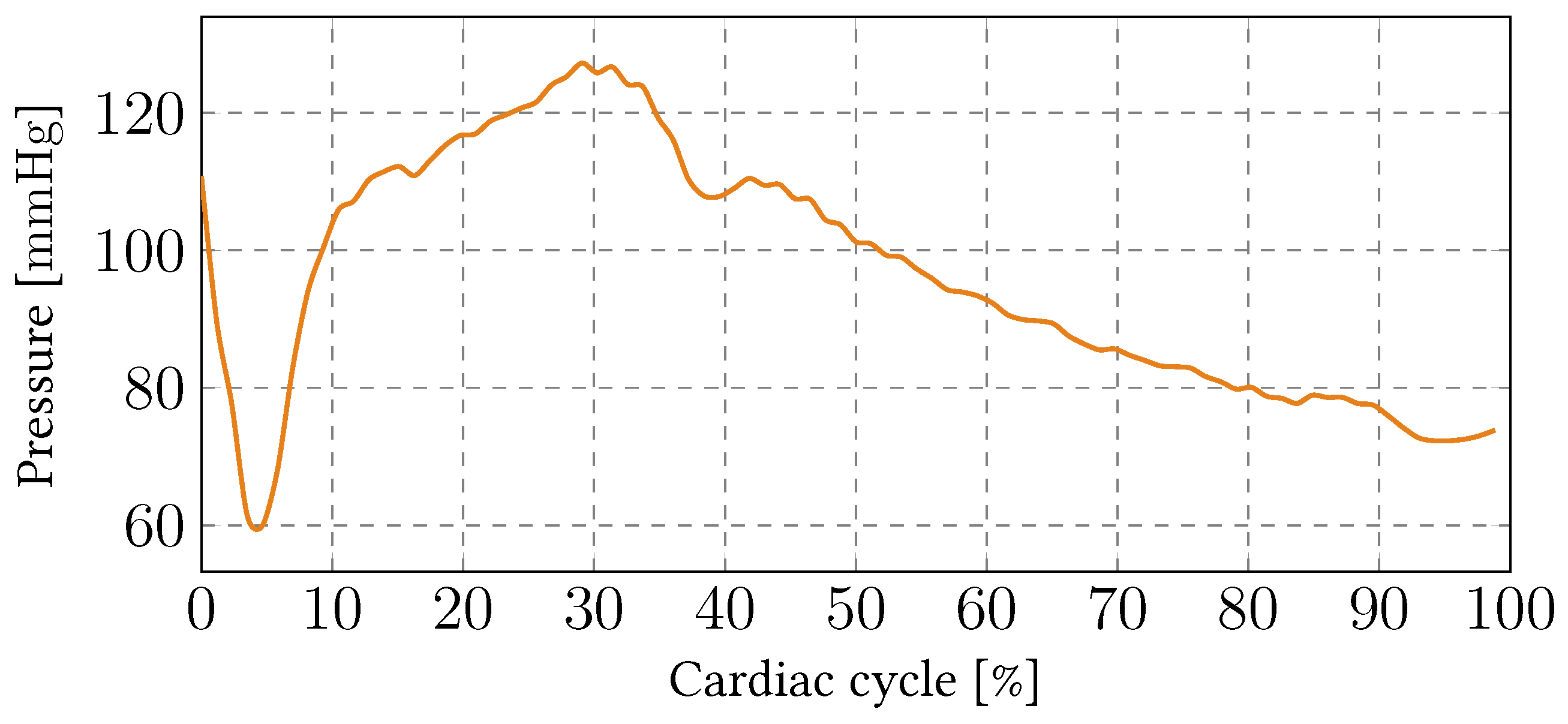
2.3. Boundary Conditions

The boundary conditions in the fluid domain were defined with a velocity inlet and impedance-based boundary conditions at the outlets. The inlet conditions were defined with a flow rate as shown in Figure 1. The spatial profile was simplified as a parabolic distribution.
The outlet boundary conditions were defined with three-element Windkessel models, also known as RCR models. These models scale the pressures and blood flow at the outlet by taking into account the impedance imposed by downstream vasculatures [58].
The values of each RCR model component for each outlet are reported in Table 2. These components were iteratively tuned to fit a typical pressure curve between 70 mmHg (diastole) and 120 mmHg (systole).
The wall at the inlet and outlets were assigned with a fixed displacement (Dirichlet boundary condition).
The aorta is always subjected to mechanical stresses throughout the cardiac cycle. In this sense, the in vivo geometry extracted from Computed Tomography scan (CT) corresponds to a deformed state within the cardiac cycle of ATAA. Assigning a prestress is a method of accounting for the in vivo stress state related to the patient-specific 3D geometric reconstruction from the CT scan.
Bäumler et al. [57] mentioned two prestress methods that lead to similar results. We used the methodology presented in Figure 2. This starts with a CFD analysis on the Luminal Domain (LD), followed by a structural analysis in the Solid Domain (SD) with the pressure of the previous phase as a boundary condition. Hsu and Bazilevs [59] develop a similar approach but with a fluid traction vector instead of a pressure distribution. Afterwards, both results from CFD and CSM are implemented as an initial condition.
Fonken et al. [60] mentioned that the FSI model with prestress can effectively reach a stable state within a single cardiac cycle. Nonetheless, future analyses are still needed to verify this statement.

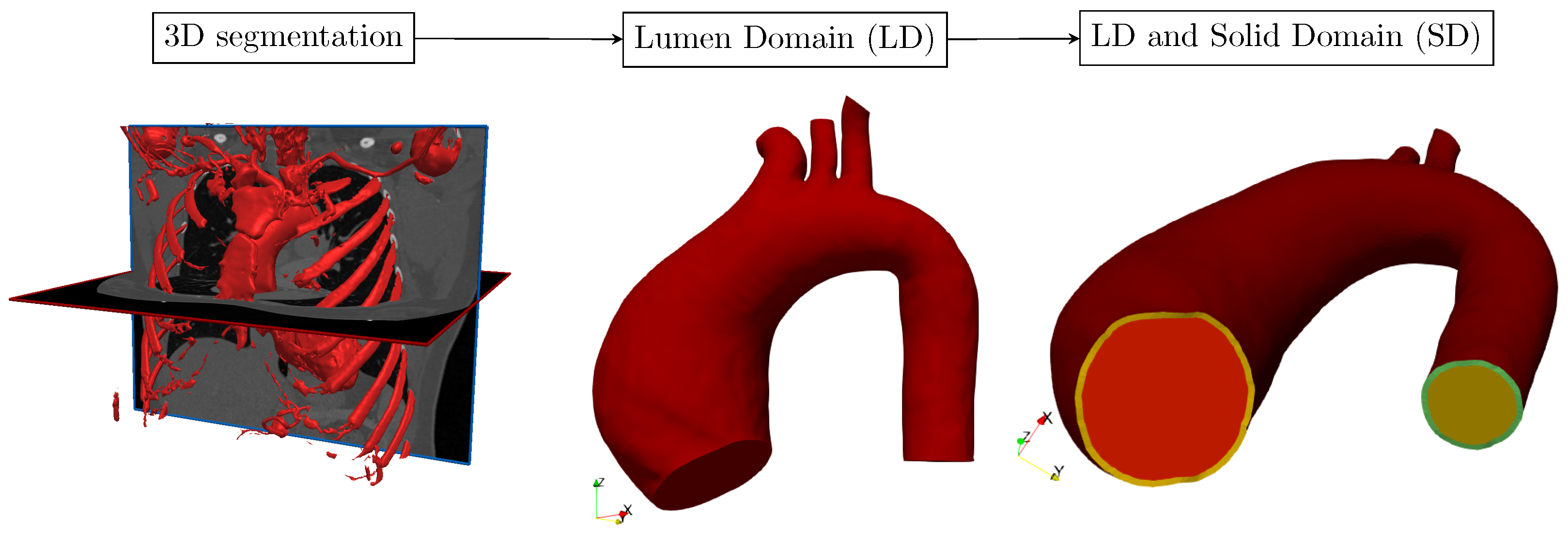
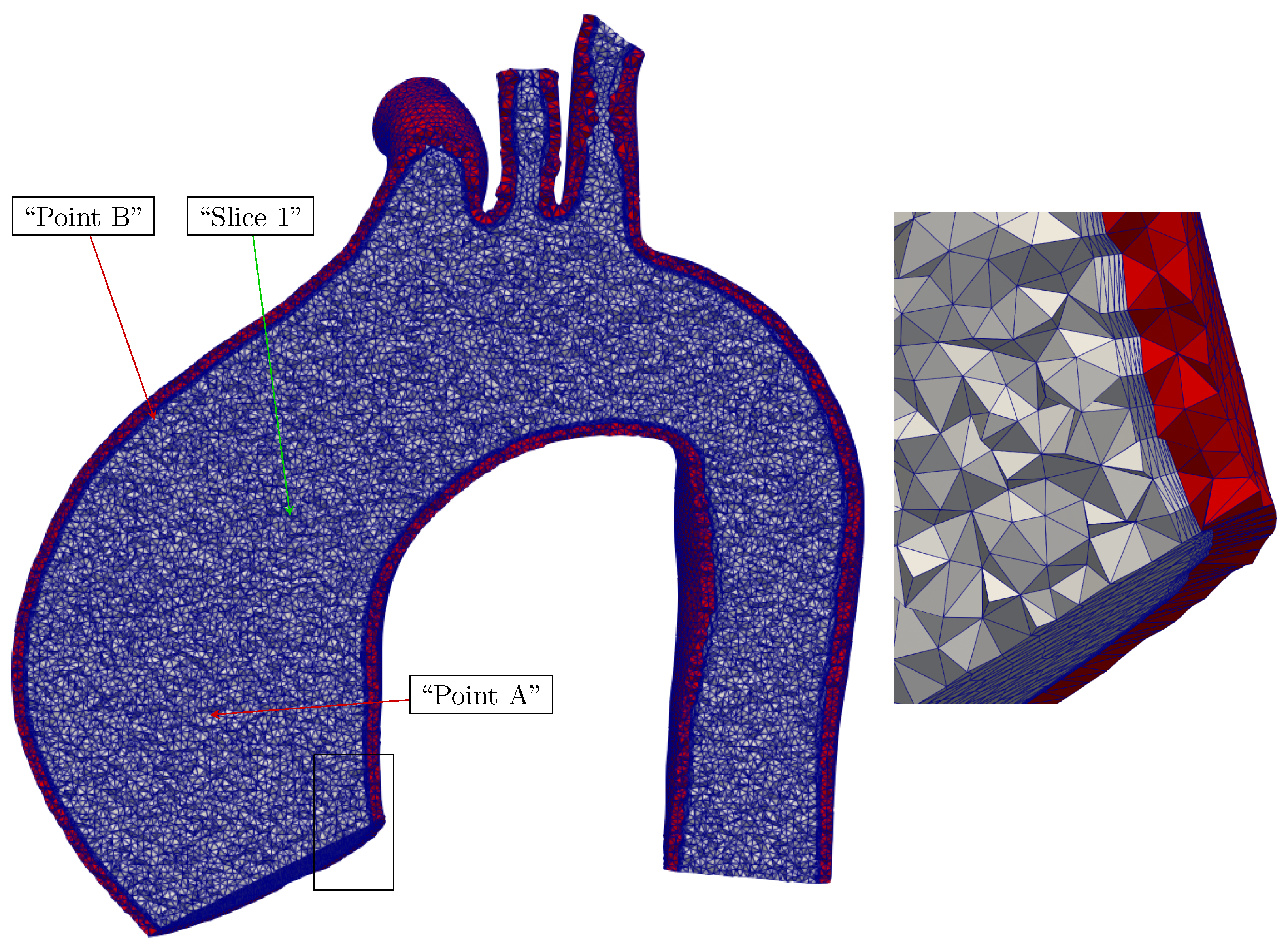
2.4. Mesh Development Workflow in SimVascular

The geometric model was split into two domains: the SD and the LD. Figure 3 shows the workflow for preparing both domains. First, we extract the LD from the CT scan of a patient with MITK Segmentation (developed by VMTK and incorporated in SimVascular). This tool was used to generate a surface mesh based on the pixel intensity with a threshold between 341 and 1706. This threshold interval was chosen through an interactive process using the two-dimensional mesh preview in SimVascular. Cleaning and filtering were performed using the Blender open source mesh editing tool.
In SimVascular, the SD is usually reconstructed from the LD concentric mesh (the boundary layer). Here, we introduced another approach without using the LD mesh, hence decoupling the element size from both domains (last step of Figure 3). In this approach, the SD was developed by extruding the outer surface of the LD in a mesh editing software (Blender) with a constant thickness of 1.5 m m [61].
SimVascular also allows the construction of finite-element meshes with unstructured tetrahedral elements using a library TetGen. However, it is essential at this stage not to change the interface mesh, as there must be consistency between the outer surface of the LD and the inner surface of the SD. Figure 4 shows the mesh using the second method. The mesh structure of both SD and LD remained unchanged regardless of the element size used in the mesh sensitivity analysis. It is worth noting that the SD mesh consists of two layers in the radial direction.
To perform mesh optimization and verify the mesh convergence, a mesh sensitivity analysis was performed in two phases. The first phase consisted of decreasing the SD volumetric element size while the LD remained constant. This procedure called “SD mesh size variation” was carried out until the difference between two successive results. Afterwards, in the second phase, the same process was performed for the LD element size with the name “LD mesh size variation”. Both phases were performed within the first 300 m s of the cardiac cycle. All numerical calculations were carried out with a Xeon(R) Gold 6230R CPU (two processors).
We paid special attention to the results obtained at two points and a slice within the Region of interest (ROI) shown in Figure 4. “Point A” located in the centerline in the middle of ATAA was used to verify the convergence of the velocity over time; “Point B” located in the inner aortic wall outer curvature was used to evaluate the convergence of WSS; and “Slice 1”, which is perpendicular to the centerline and passes through Points “A” and “B”, was used to evaluate the convergence of the cross-section area variation. We computed the Normalized Amplitude Error (NAE), A χ , and the Normalized Phase Amplitude Error (NPAE), φ χ as defined in Equations (8) and (9), respectively.
A χ = i = 1 n χ i 2 i = 1 n χ i ref 2
φ χ = i = 1 n χ i χ i ref 2 i = 1 n χ i ref 2
where χ i is the quantity of interest, χ i ref is its reference value (corresponding to the most refined mesh), and n is the time spatial resolution within the cardiac cycle. The mesh sensitivity analysis is considered converged if both NAE and NPAE are within a small percentage of consecutive results.

3. Results

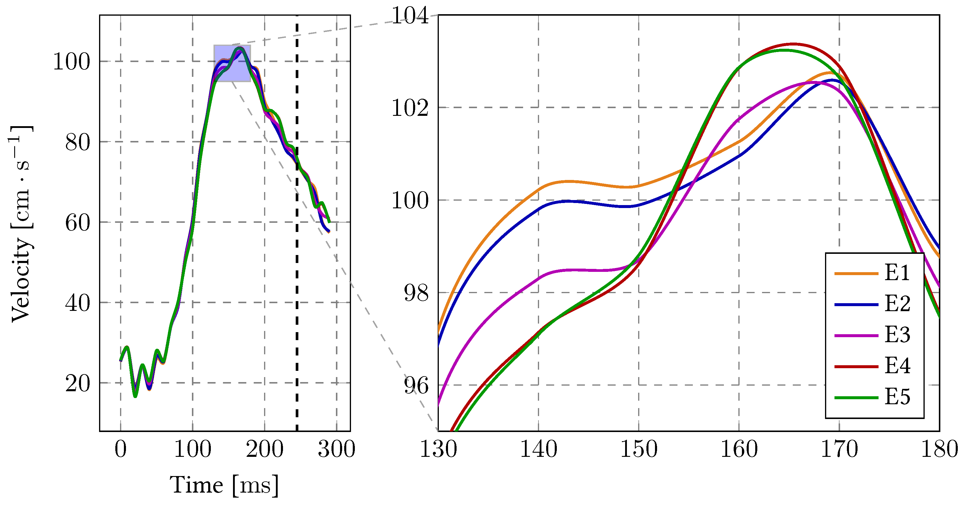
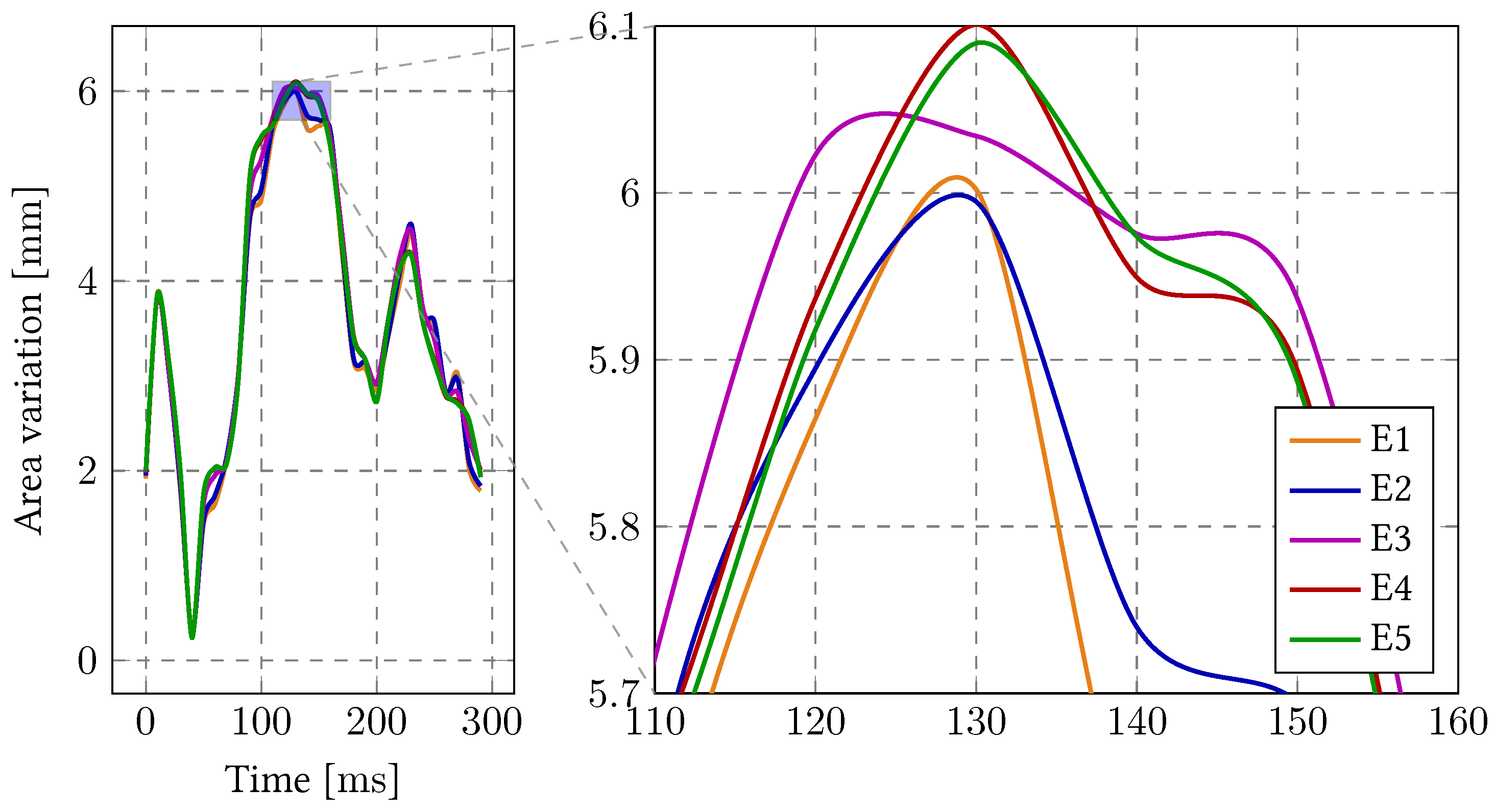
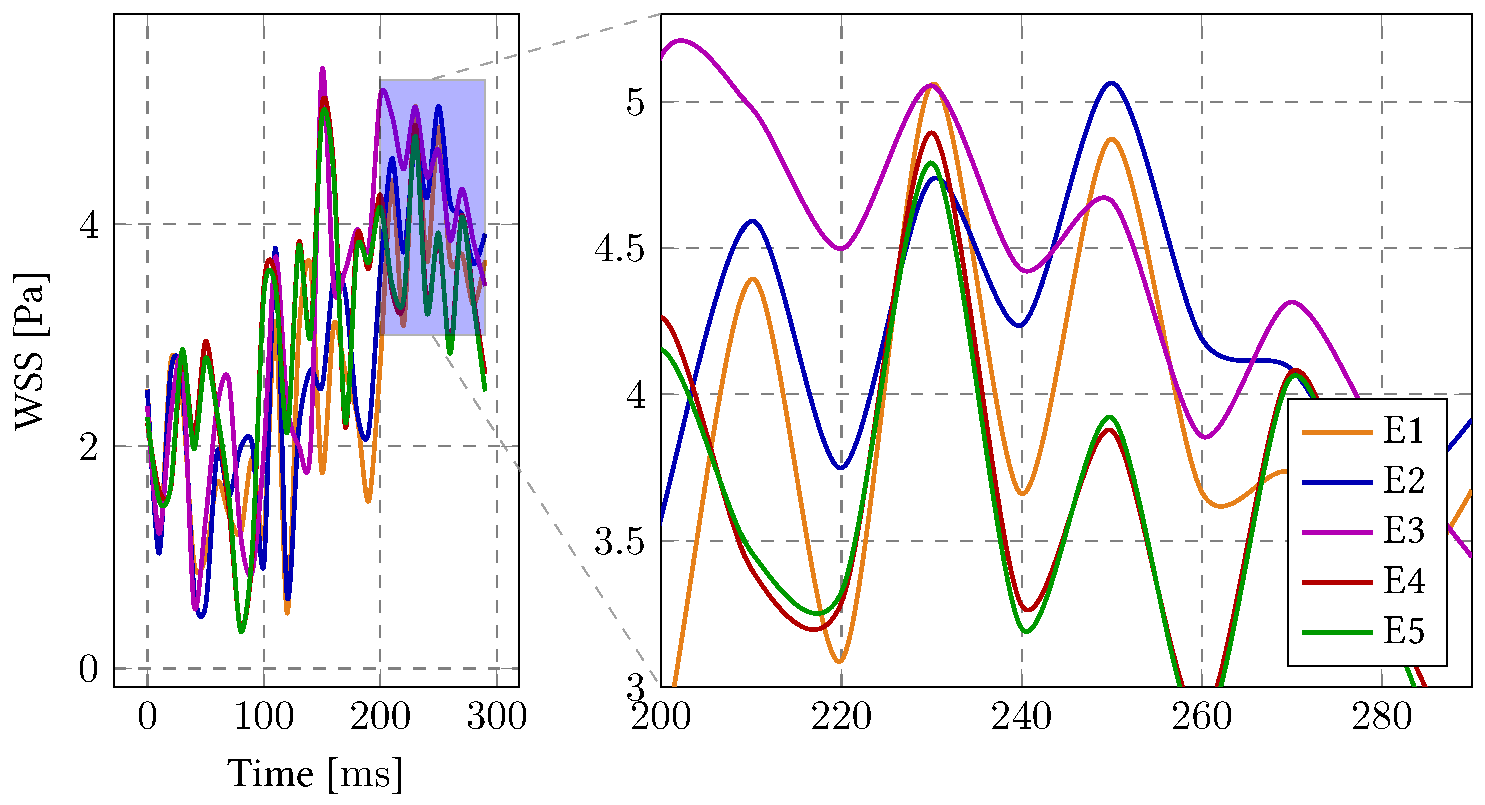
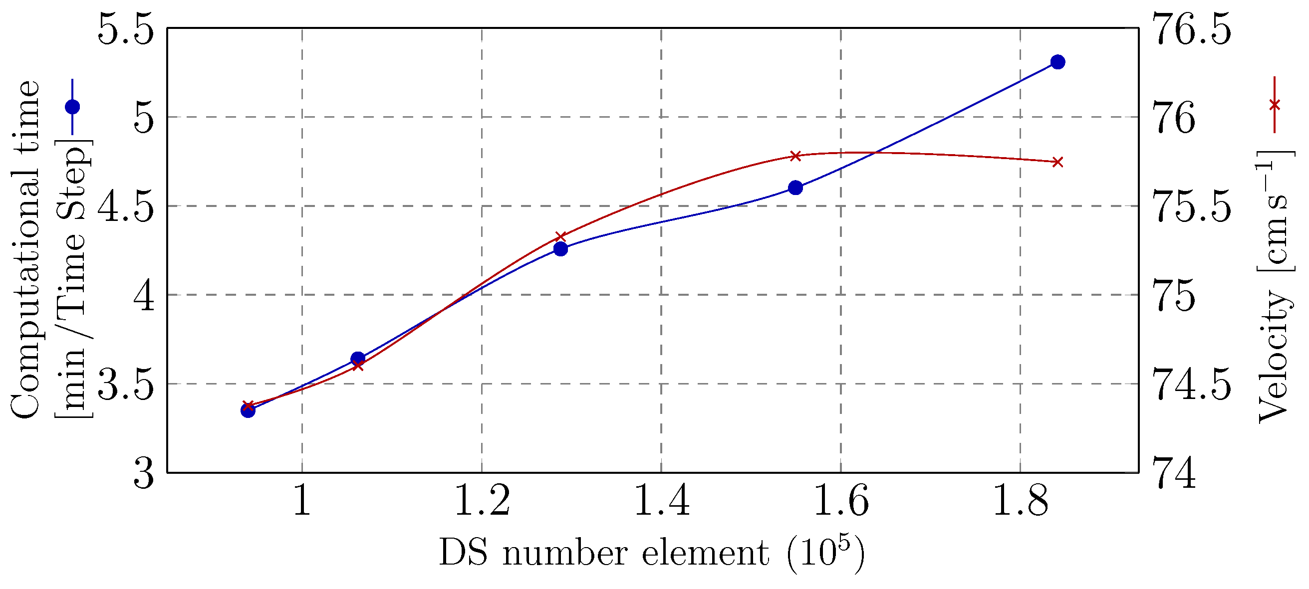
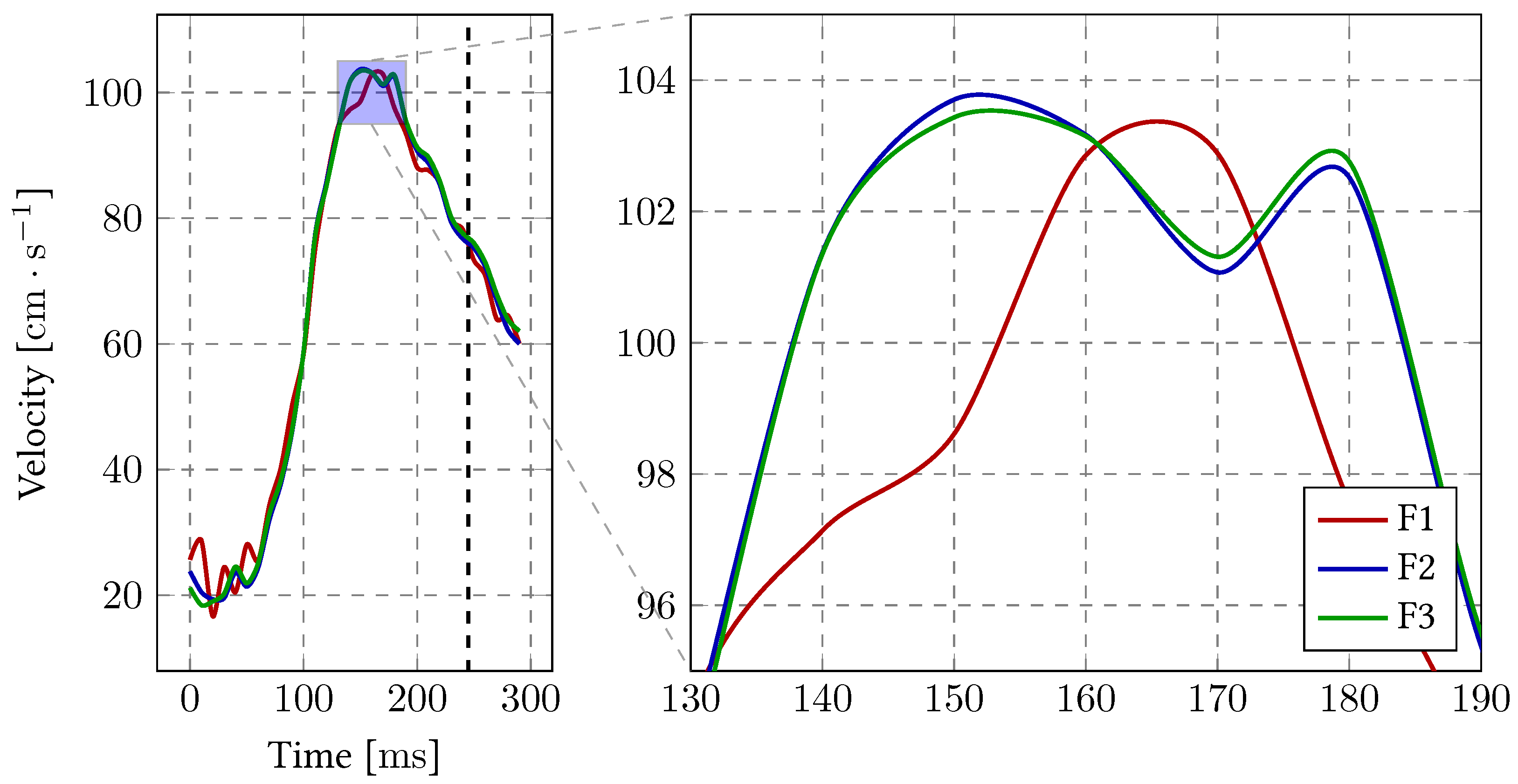
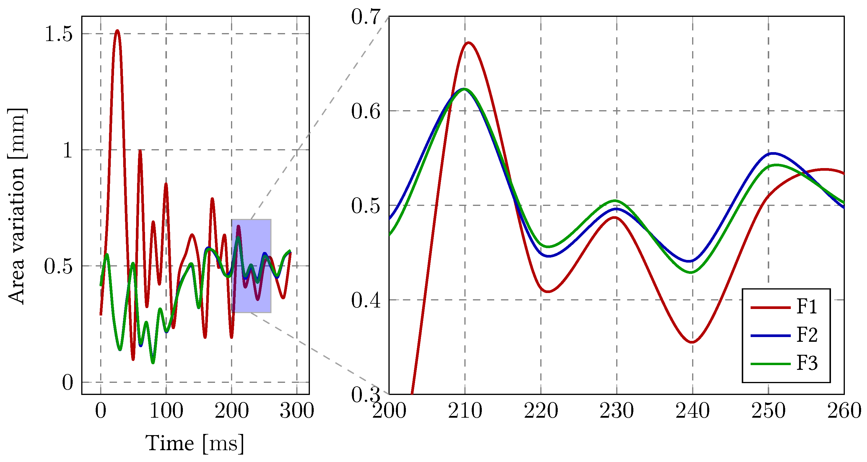
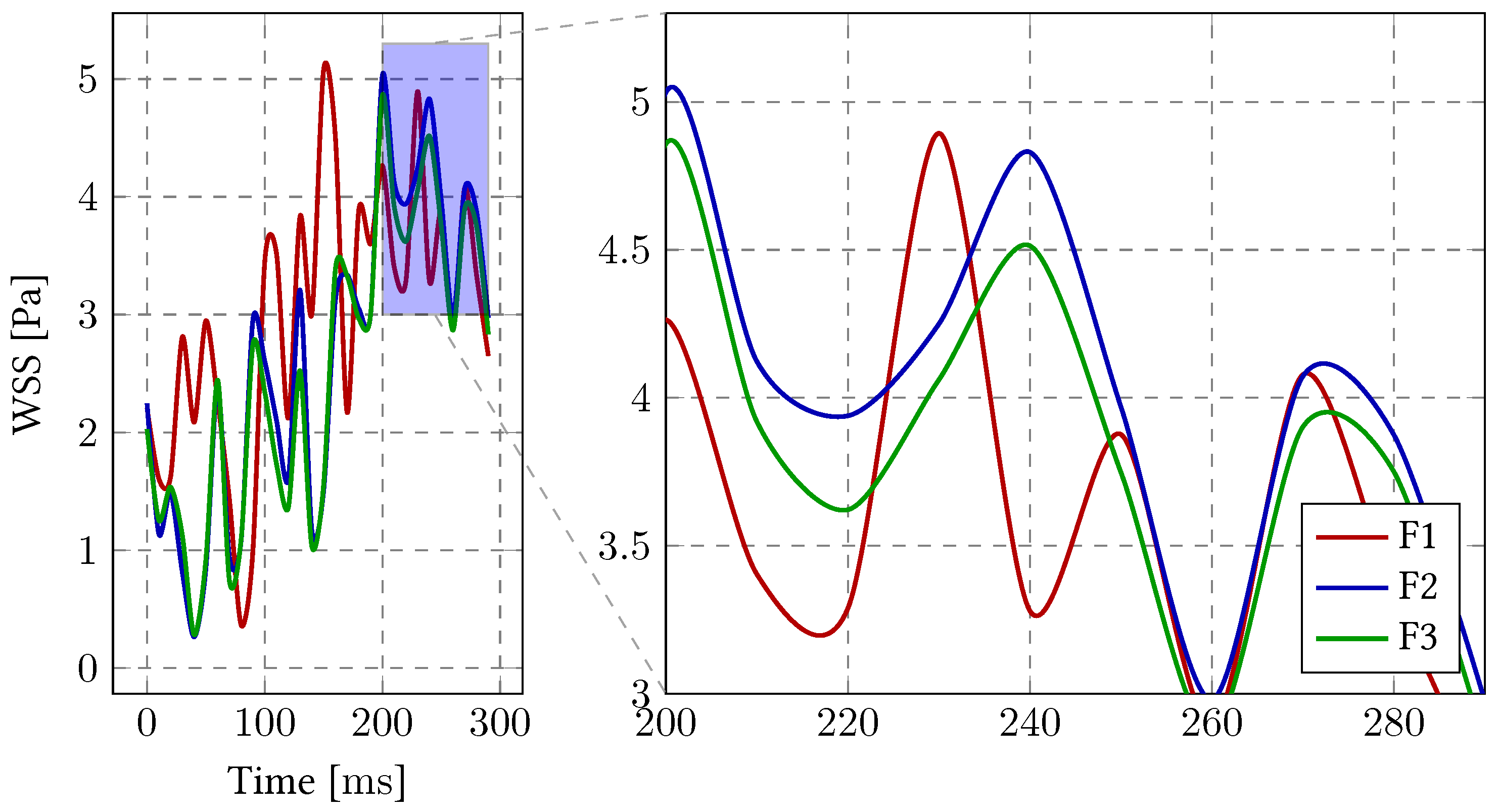
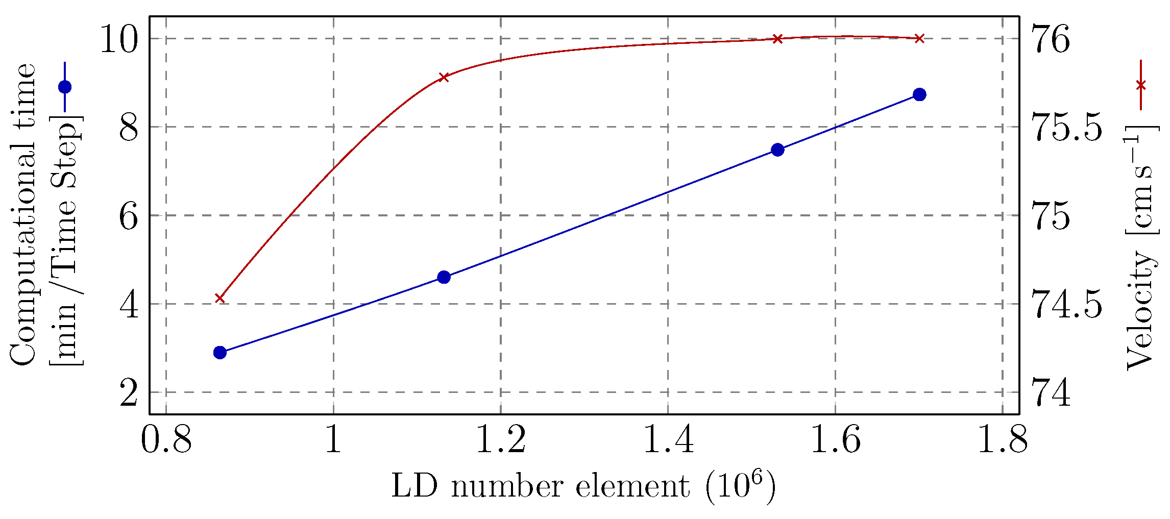
3.1. Sensitivity Analysis

Table 3 shows element sizes for each numerical model in the “SD mesh size variation”.
Figure 5, Figure 6 and Figure 7 show variations of the velocity at “Point A”, area variation from “Slice 1” and the WSS at “Point B”, respectively. This reveals the relatively low impact of the DS mesh on hemodynamics and wall motion, and the good agreement between the numerical models “E4” and “E5”.
Table 4 shows the NAE, A χ , and the NPAE, φ χ , calculated with all previous simulations regarding the “SD mesh size variation”. This method allows a quantitative analysis regarding the convergence of those numerical models.
Both NAE and NPAE are a difference lower than 1 % in the “E4” model. It can be concluded that there is a convergence between these numerical models; therefore, it is not necessary to reduce volumetric element size.
Figure 8 shows the effect of the SD mesh size on the velocity at time instant 245 m s and related it to the computational effort (number of elements in SD). The computational time increases almost linearly with the number of elements and the velocity at “Point A” converges for the largest number of elements. Although other factors may invalidate the systematic use of the average computational time as an indicator, the significant difference between analyses shows a mesh size impact. Therefore, the optimal SD mesh is close to 1.5 × 10 5 elements, which is equivalent to the “E4” mesh.
The sensitivity to the LD mesh size was analysed with the same methodology as the previous, starting from “F1” (the previous “E4” model).
The interface mesh sensitivity was included in this analysis. The number of elements varied in the SD as in the LD outer wall (interface) mesh used to generate the SD surface mesh in our approach, as shown in Table 5.
Figure 9, Figure 10 and Figure 11 show the variation of the velocity at "Point A”, area variation in “Slice 1” and WSS at “Point B” over the computed time, respectively. There is no significant difference between “F3” and “F4”, demonstrating mesh convergence.
From these previous results, we can derive the NAE and NPAE reported in Table 6. As shown, the model “F2” is within 2.5 % , which is acceptable.
Figure 12 shows a linear increase in computational time with the size of the elements, and in parallel, there was a convergence of the velocity as expected for this time instance. This shows that the best mesh from the point of view of computational efficiency is “F2”. In summary, the best element size is 1.35   m m in the LD and 1.1   m m in the SD.

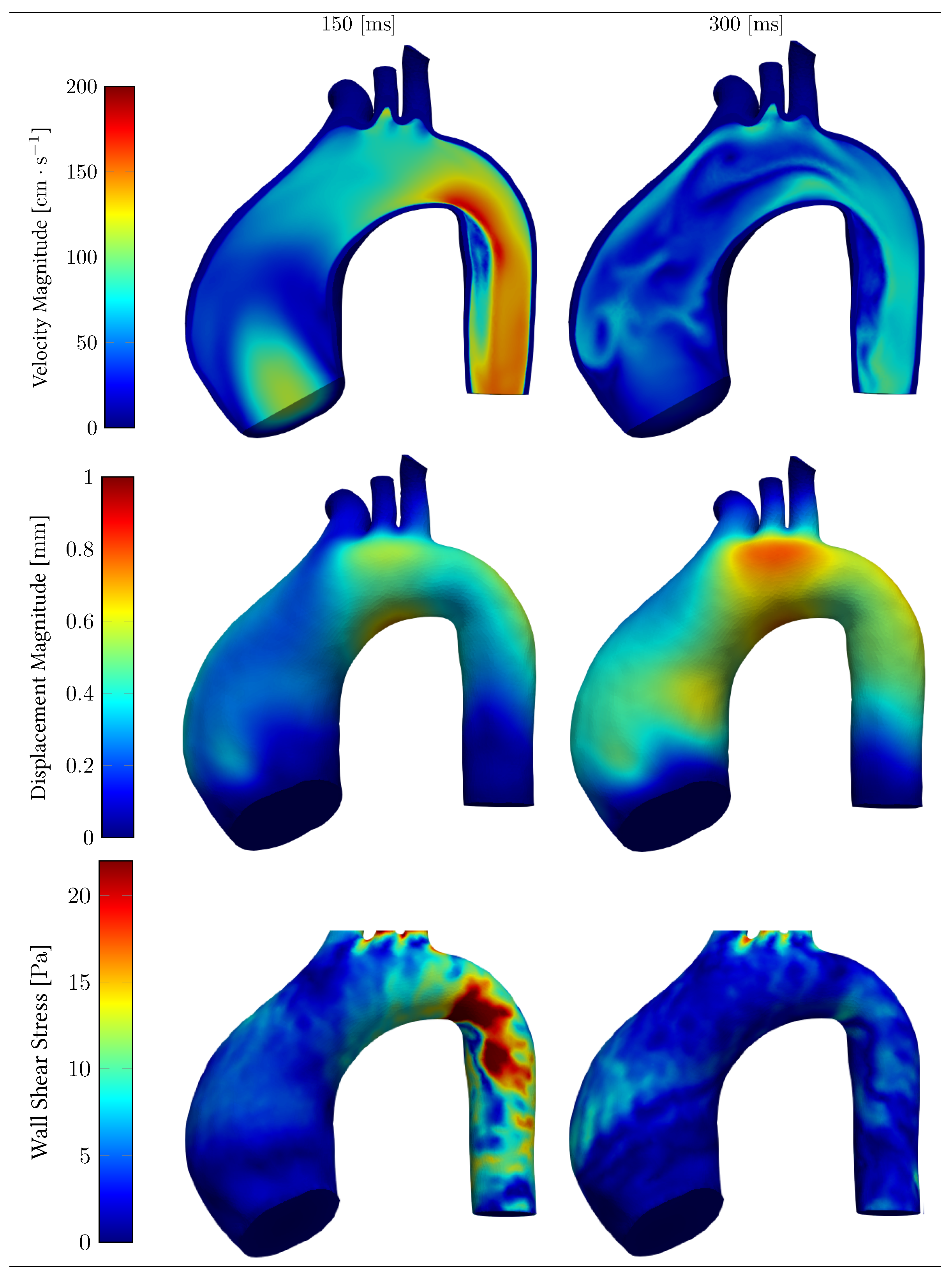
3.2. Hemodynamics and Structural Capabilities

To understand the behaviour and results capabilities, we analysed the hemodynamics and the structural behaviour in ATAA. Figure 13 shows both the velocity and displacement magnitudes and the WSS distribution within the first cardiac cycle at 150 and 300 m s (systole and beginning of diastole, respectively).
Figure 14 presents the pressure distribution inside the ATAA (“Point A”). Pressure variation ranging between 123.7 and 62.1 , as predicted, highlights the behaviour of the RCR model.

4. Discussion

Computational analyses using different approaches have been proposed in the literature as a tool to model the biomechanical behaviour of the aneurysmatic aorta to evaluate the risk of rupture and aneurism growth and progression, eventually with positive results. It has been demonstrated that the interaction between the aorta hyperelastic behaviour and hemodynamics cannot be ignored while analysing ATAA [45]. Therefore, some studies have also integrated FSI to enhance the computational models to a digital twin representation of aortic aneurysm. Nevertheless, a FSI model requires significant computational effort, especially when coupled with the three-element Windkessel model and with a prestress model [57,59].
In this work, a new method for mesh generation in SimVascular was proposed, allowing the optimization of both the fluid and solid domains in two ways. On the one hand, this allows a refined concentric mesh next to the LD outside wall. This mesh section was optimized to efficiently resolve the boundary layer and consequently allow a coarser increase in element size in the remaining domain. On the other hand, this methodology yielded the element size optimization in each domain which was almost independent, leading to a more efficient mesh sensitivity analysis, and improving the number of mesh elements. Both these improvements lead to a coarser mesh, without a loss of accuracy, thus guaranteeing a reduction in computational time.
The RCR model applied ranging between 123.7 mmHg and 62.1 mmHg. These pressure variation values meet the iterative process used to develop the RCR model. Furthermore, the pressure starts in a non-resting state, showing the significance of the initial condition. The pressure difference, between the first and last time steps of the cardiac cycle, shows a non-periodicity in our model. Further analysis needed to be performed to fully understand the cycle-to-cycle periodicity.
To validate the in silico capability in the numerical model results would require further patient-specific analysis. However, simplification regarding the limit state of the incoming space vector flow and wall properties may play a significant role in predicting results on ATAA. This assumption is based on the relationship between ATAA and pathologies responsible for altered hemodynamics such as that observed in BAV [7,62,63]. The present numerical model can be improved by including the variation in ATAA thickness and improving both the estimation of tissue mechanical properties and patient-specific boundary conditions. Moreover, the numerical model can be further validated by using 4D-MRI to analyse the AD progression.
Fonken et al. [60] demonstrated that, after three cardiac cycles, there are some resemblances in the pressure and flow between the model without prestress and the first cardiac cycle of a model with prestress. In this sense, there may be convergence in the model with prestress after a single cardiac cycle and both models may have a similar result. Furthermore, they mention that this analysis was not performed due to a lack of computational time. Further analysis must be performed to fully conclude the convergence possibility. Further studies may focus on improving the numerical model, verifying the prestress significance in the model, and validating the first cardiac cycle results against cycle-to-cycle analyses.

5. Conclusions

This work addresses an FSI simulation of the ATAA using the SimVascular open access software A considerable computational time of approximately 100 h in a workstation was typically required. The computational cost was mitigated by improving the efficiency in meshing creation and convergence in both fluid and solid domains. In future work, we plan to improve the prestress and Windkessel models. The verification of the convergence across cycle-to-cycle analyses will also be performed. Moreover, the numerical model will be compared against in vivo measurements based on 4D MRI for validation.

Author Contributions

Conceptualization, R.V., A.M., M.B., J.X., A.T. and S.A.; methodology, R.V., A.M., M.B., J.X., A.T. and S.A.; software, R.V., A.M., M.B., J.X. and A.T.; validation, R.V., A.M., M.B., J.X., A.T. and S.A.; formal analysis, R.V., A.M., M.B., J.X., A.T. and S.A.; investigation, R.V., A.M., M.B., J.X., A.T. and S.A.; resources, M.B. and J.X.; writing—original draft preparation, R.V., A.M., M.B. and J.X.; writing—review and editing, R.V., A.M., M.B., J.X., A.T. and S.A.; visualization, R.V., A.M., M.B. and J.X.; supervision, M.B., J.X. and S.A.; project administration, J.X.; funding acquisition, J.X. All authors have read and agreed to the published version of the manuscript.

Funding

Portuguese Foundation for Science and Technology (FCT) under the project PTDC/EMD-EMD/1230/2021 “Fluid–structure interaction for functional assessment of ascending aortic aneurysms: a biomechanical-based approach toward clinical practice”, and UIDB/00667/2020 (UNIDEMI). A. Mourato is also grateful to the FCT for the Ph.D. grant UI/BD/151212/2021.

Institutional Review Board Statement

Not applicable.

Informed Consent Statement

Informed consent was obtained from all subjects involved in the study.

Data Availability Statement

Not applicable.

Conflicts of Interest

The authors declare no conflict of interest.

Abbreviations

The following abbreviations are used in this manuscript:
ADAortic Dissection
ALEArbitrary Lagrangian–Eulerian
AIArtificial Intelligence
ATAAAscending Thoracic Aortic Aneurysm
CSMComputational Solid Mechanics
CFDComputational Fluid Dynamics
CTComputed Tomography scan
ESCEuropean Society of Cardiology
FSIFluid–Structure Interaction
LDLuminal Domain
MRIMagnetic Resonance Imaging
NAENormalized Amplitude Error
NPAENormalized Phase Amplitude Error
ROIRegion of Interest
SDSolid Domain
WSSWall Shear Stress
FEMFinite Element Method
FEAFinite Element Analysis
BAVBicuspid Aortic Valve

References

  1. Dieter, R.; Dieter, R.; Dieter, R., III. Diseases of the Aorta; Springer: Berlin/Heidelberg, Germany, 2019. [Google Scholar] [CrossRef]
  2. Pasta, S.; Rinaudo, A.; Luca, A.; Pilato, M.; Scardulla, C.; Gleason, T.G.; Vorp, D.A. Difference in hemodynamic and wall stress of ascending thoracic aortic aneurysms with bicuspid and tricuspid aortic valve. J. Biomech. 2013, 46, 1729–1738. [Google Scholar] [CrossRef] [PubMed] [Green Version]
  3. Erbel, R.; Aboyans, V.; Boileau, C.; Bossone, E.; Bartolomeo, R.D.; Eggebrecht, H.; Evangelista, A.; Falk, V.; Frank, H.; Gaemperli, O.; et al. 2014 ESC guidelines on the diagnosis and treatment of aortic diseases. Eur. Heart J. 2014, 35, 2873–2926. [Google Scholar] [CrossRef] [Green Version]
  4. Maiti, S.; Thunes, J.R.; Fortunato, R.N.; Gleason, T.G.; Vorp, D.A. Computational modeling of the strength of the ascending thoracic aortic media tissue under physiologic biaxial loading conditions. J. Biomech. 2020, 108, 109884. [Google Scholar] [CrossRef]
  5. Farzaneh, S.; Trabelsi, O.; Avril, S. Inverse identification of local stiffness across ascending thoracic aortic aneurysms. Biomech. Model. Mechanobiol. 2019, 18, 137–153. [Google Scholar] [CrossRef] [PubMed]
  6. Trimarchi, S.; Jonker, F.H.; Hutchison, S.; Isselbacher, E.M.; Pape, L.A.; Patel, H.J.; Froehlich, J.B.; Muhs, B.E.; Rampoldi, V.; Grassi, V.; et al. Descending aortic diameter of 5.5 cm or greater is not an accurate predictor of acute type B aortic dissection. J. Thorac. Cardiovasc. Surg. 2011, 142, e101–e107. [Google Scholar] [CrossRef] [PubMed] [Green Version]
  7. Youssefi, P.; Sharma, R.; Figueroa, C.A.; Jahangiri, M. Functional assessment of thoracic aortic aneurysms—The future of risk prediction? Br. Med. Bull. 2017, 121, 61–71. [Google Scholar] [CrossRef] [Green Version]
  8. Gzik-Zroska, B.; Joszko, K.; Wolański, W.; Gzik, M. Development of New Testing Method of Mechanical Properties of Porcine Coronary Arteries. In Information Technologies in Medicine; Piętka, E., Badura, P., Kawa, J., Wieclawek, W., Eds.; Advances in Intelligent Systems and Computing; Springer International Publishing: Berlin/Heidelberg, Germany, 2016; Volume 472, pp. 289–297. [Google Scholar] [CrossRef]
  9. Youssefi, P.; Gomez, A.; He, T.; Anderson, L.; Bunce, N.; Sharma, R.; Figueroa, C.A.; Jahangiri, M. Patient-specific computational fluid dynamics—Assessment of aortic hemodynamics in a spectrum of aortic valve pathologies. J. Thorac. Cardiovasc. Surg. 2017, 153, 8–20.e3. [Google Scholar] [CrossRef] [Green Version]
  10. Mourato, A.; Brito, M.; Xavier, J.; Gil, L.; Tomás, A. On the RANS modelling of the patient-specific thoracic aortic aneurysm. In Advances and Current Trends in Biomechanics; CRC Press: Boca Raton, FL, USA, 2021; pp. 98–102. [Google Scholar]
  11. Shang, E.K.; Nathan, D.P.; Sprinkle, S.R.; Vigmostad, S.C.; Fairman, R.M.; Bavaria, J.E.; Gorman, R.C.; Gorman, J.H., III; Chandran, K.B.; Jackson, B.M. Peak wall stress predicts expansion rate in descending thoracic aortic aneurysms. Ann. Thorac. Surg. 2013, 95, 593–598. [Google Scholar] [CrossRef] [Green Version]
  12. Gültekin, O.; Hager, S.P.; Dal, H.; Holzapfel, G.A. Computational modeling of progressive damage and rupture in fibrous biological tissues: Application to aortic dissection. Biomech. Model. Mechanobiol. 2019, 18, 1607–1628. [Google Scholar] [CrossRef] [Green Version]
  13. Mousavi, S.J.; Jayendiran, R.; Farzaneh, S.; Campisi, S.; Viallon, M.; Croisille, P.; Avril, S. Coupling hemodynamics with mechanobiology in patient-specific computational models of ascending thoracic aortic aneurysms. Comput. Methods Programs Biomed. 2021, 205, 106107. [Google Scholar] [CrossRef]
  14. Taghizadeh, H.; Tafazzoli-Shadpour, M.; Shadmehr, M.B. Analysis of arterial wall remodeling in hypertension based on lamellar modeling. J. Am. Soc. Hypertens. 2015, 9, 735–744. [Google Scholar] [CrossRef] [PubMed]
  15. Liu, M.; Liang, L.; Sun, W. Estimation of in vivo mechanical properties of the aortic wall: A multi-resolution direct search approach. J. Mech. Behav. Biomed. Mater. 2018, 77, 649–659. [Google Scholar] [CrossRef] [PubMed]
  16. Thunes, J.R.; Phillippi, J.A.; Gleason, T.G.; Vorp, D.A.; Maiti, S. Structural modeling reveals microstructure-strength relationship for human ascending thoracic aorta. J. Biomech. 2018, 71, 84–93. [Google Scholar] [CrossRef] [PubMed]
  17. Capellini, K.; Vignali, E.; Costa, E.; Gasparotti, E.; Biancolini, M.E.; Landini, L.; Positano, V.; Celi, S. Computational fluid dynamic study for aTAA hemodynamics: An integrated image-based and radial basis functions mesh morphing approach. J. Biomech. Eng. 2018, 140, 111007. [Google Scholar] [CrossRef]
  18. Thunes, J.R.; Pal, S.; Fortunato, R.N.; Phillippi, J.A.; Gleason, T.G.; Vorp, D.A.; Maiti, S. A structural finite element model for lamellar unit of aortic media indicates heterogeneous stress field after collagen recruitment. J. Biomech. 2016, 49, 1562–1569. [Google Scholar] [CrossRef] [Green Version]
  19. Ban, E.; Cavinato, C.; Humphrey, J.D. Differential propensity of dissection along the aorta. Biomech. Model. Mechanobiol. 2021, 20, 895–907. [Google Scholar] [CrossRef]
  20. Wang, R.; Yu, X.; Gkousioudi, A.; Zhang, Y. Effect of Glycation on Interlamellar Bonding of Arterial Elastin. Exp. Mech. 2021, 61, 81–94. [Google Scholar] [CrossRef]
  21. Mousavi, S.J.; Farzaneh, S.; Avril, S. Patient-specific predictions of aneurysm growth and remodeling in the ascending thoracic aorta using the homogenized constrained mixture model. Biomech. Model. Mechanobiol. 2019, 18, 1895–1913. [Google Scholar] [CrossRef] [Green Version]
  22. Hackstein, U.; Krickl, S.; Bernhard, S. Estimation of ARMA-model parameters to describe pathological conditions in cardiovascular system models. Inform. Med. Unlocked 2020, 18, 100310. [Google Scholar] [CrossRef]
  23. Adam, C.; Fabre, D.; Mougin, J.; Zins, M.; Azarine, A.; Ardon, R.; d’Assignies, G.; Haulon, S. Pre-surgical and Post-surgical Aortic Aneurysm Maximum Diameter Measurement: Full Automation by Artificial Intelligence. Eur. J. Vasc. Endovasc. Surg. 2021, 62, 869–877. [Google Scholar] [CrossRef]
  24. Cao, L.; Shi, R.; Ge, Y.; Xing, L.; Zuo, P.; Jia, Y.; Liu, J.; He, Y.; Wang, X.; Luan, S.; et al. Fully automatic segmentation of type B aortic dissection from CTA images enabled by deep learning. Eur. J. Radiol. 2019, 121, 108713. [Google Scholar] [CrossRef]
  25. Sazonov, I.; Xie, X.; Nithiarasu, P. An improved method of computing geometrical potential force (GPF) employed in the segmentation of 3D and 4D medical images. Comput. Methods Biomech. Biomed. Eng. Imaging Vis. 2017, 5, 287–296. [Google Scholar] [CrossRef]
  26. Rueckel, J.; Reidler, P.; Fink, N.; Sperl, J.; Geyer, T.; Fabritius, M.; Ricke, J.; Ingrisch, M.; Sabel, B. Artificial intelligence assistance improves reporting efficiency of thoracic aortic aneurysm CT follow-up. Eur. J. Radiol. 2021, 134, 109424. [Google Scholar] [CrossRef] [PubMed]
  27. He, X.; Avril, S.; Lu, J. Prediction of local strength of ascending thoracic aortic aneurysms. J. Mech. Behav. Biomed. Mater. 2021, 115, 104284. [Google Scholar] [CrossRef]
  28. Lindquist Liljeqvist, M.; Bogdanovic, M.; Siika, A.; Gasser, T.C.; Hultgren, R.; Roy, J. Geometric and biomechanical modeling aided by machine learning improves the prediction of growth and rupture of small abdominal aortic aneurysms. Sci. Rep. 2021, 11, 18040. [Google Scholar] [CrossRef]
  29. Liu, M.; Liang, L.; Sun, W. Estimation of in vivo constitutive parameters of the aortic wall using a machine learning approach. Comput. Methods Appl. Mech. Eng. 2019, 347, 201–217. [Google Scholar] [CrossRef] [PubMed]
  30. Holzapfel, G.A.; Linka, K.; Sherifova, S.; Cyron, C.J. Predictive constitutive modelling of arteries by deep learning. J. R. Soc. Interface 2021, 18, 20210411. [Google Scholar] [CrossRef] [PubMed]
  31. Liu, J.; Yang, W.; Lan, I.S.; Marsden, A.L. Fluid–structure interaction modeling of blood flow in the pulmonary arteries using the unified continuum and variational multiscale formulation. Mech. Res. Commun. 2020, 107, 103556. [Google Scholar] [CrossRef]
  32. Liang, L.; Liu, M.; Martin, C.; Sun, W. A machine learning approach as a surrogate of finite element analysis–based inverse method to estimate the zero-pressure geometry of human thoracic aorta. Int. J. Numer. Methods Biomed. Eng. 2018, 34, e3103. [Google Scholar] [CrossRef] [PubMed]
  33. Liang, L.; Liu, M.; Martin, C.; Sun, W. A deep learning approach to estimate stress distribution: A fast and accurate surrogate of finite-element analysis. J. R. Soc. Interface 2018, 15, 20170844. [Google Scholar] [CrossRef] [Green Version]
  34. Zhang, Y.; Lu, Q.; Feng, J.; Yu, P.; Zhang, S.; Teng, Z.; Gillard, J.H.; Song, R.; Jing, Z. A pilot study exploring the mechanisms involved in the longitudinal propagation of acute aortic dissection through computational fluid dynamic analysis. Cardiology 2014, 128, 220–225. [Google Scholar] [CrossRef] [PubMed]
  35. Long Ko, J.K.; Liu, R.W.; Ma, D.; Shi, L.; Ho Yu, S.C.; Wang, D. Pulsatile hemodynamics in patient-specific thoracic aortic dissection models constructed from computed tomography angiography. J. X-ray Sci. Technol. 2017, 25, 233–245. [Google Scholar] [CrossRef]
  36. Kaspera, W.; Ćmiel Smorzyk, K.; Wolański, W.; Kawlewska, E.; Hebda, A.; Gzik, M.; Ładziński, P. Morphological and Hemodynamic Risk Factors for Middle Cerebral Artery Aneurysm: A Case-Control Study of 190 Patients. Sci. Rep. 2020, 10, 2016. [Google Scholar] [CrossRef]
  37. Pasta, S.; Agnese, V.; Gallo, A.; Cosentino, F.; Di Giuseppe, M.; Gentile, G.; Raffa, G.M.; Maalouf, J.F.; Michelena, H.I.; Bellavia, D.; et al. Shear Stress and Aortic Strain Associations with Biomarkers of Ascending Thoracic Aortic Aneurysm. Ann. Thorac. Surg. 2020, 110, 1595–1604. [Google Scholar] [CrossRef] [PubMed]
  38. Condemi, F.; Campisi, S.; Viallon, M.; Troalen, T.; Xuexin, G.; Barker, A.; Markl, M.; Croisille, P.; Trabelsi, O.; Cavinato, C.; et al. Fluid-and biomechanical analysis of ascending thoracic aorta aneurysm with concomitant aortic insufficiency. Ann. Biomed. Eng. 2017, 45, 2921–2932. [Google Scholar] [CrossRef] [PubMed]
  39. Simão, M.; Ferreira, J.M.; Tomas, A.C.; Fragata, J.; Ramos, H.M. Aorta ascending aneurysm analysis using CFD models towards possible anomalies. Fluids 2017, 2, 31. [Google Scholar] [CrossRef] [Green Version]
  40. Tomaszewski, M.; Sybilski, K.; Małachowski, J.; Wolański, W.; Buszman, P.P. Numerical and experimental analysis of balloon angioplasty impact on flow hemodynamics improvement. Acta Bioeng. Biomech. 2020, 22, 169–183. [Google Scholar] [CrossRef]
  41. Yeh, H.H.; Rabkin, S.W.; Grecov, D. Hemodynamic assessments of the ascending thoracic aortic aneurysm using fluid–structure interaction approach. Med. Biol. Eng. Comput. 2018, 56, 435–451. [Google Scholar] [CrossRef]
  42. Chen, H.; Peelukhana, S.; Berwick, Z.; Kratzberg, J.; Krieger, J.; Roeder, B.; Chambers, S.; Kassab, G. Editor’s Choice–Fluid–Structure Interaction Simulations of Aortic Dissection with Bench Validation. Eur. J. Vasc. Endovasc. Surg. 2016, 52, 589–595. [Google Scholar] [CrossRef] [Green Version]
  43. Mendez, V.; Di Giuseppe, M.; Pasta, S.; Giuseppe, M.D.; Pasta, S. Comparison of hemodynamic and structural indices of ascending thoracic aortic aneurysm as predicted by 2-way FSI, CFD rigid wall simulation and patient-specific displacement-based FEA. Comput. Biol. Med. 2018, 100, 221–229. [Google Scholar] [CrossRef]
  44. Alimohammadi, M.; Sherwood, J.M.; Karimpour, M.; Agu, O.; Balabani, S.; Díaz-Zuccarini, V. Aortic dissection simulation models for clinical support: Fluid–structure interaction vs. rigid wall models. Biomed. Eng. Online 2015, 14, 34. [Google Scholar] [CrossRef] [PubMed] [Green Version]
  45. Zouggari, L.; Bou-said, B.; Massi, F.; Culla, A.; Millon, A. The Role of Biomechanics in the Assessment of Carotid Atherosclerosis Severity: A Numerical Approach. World J. Vasc. Surg. 2018, 1, 1007. [Google Scholar]
  46. Ateshian, G.A.; Shim, J.J.; Maas, S.A.; Weiss, J.A. Finite Element Framework for Computational Fluid Dynamics in FEBio. J. Biomech. Eng. 2018, 140, 021001. [Google Scholar] [CrossRef] [PubMed] [Green Version]
  47. Lopes, D.; Agujetas, R.; Puga, H.; Teixeira, J.; Lima, R.; Alejo, J.; Ferrera, C. Analysis of finite element and finite volume methods for fluid–structure interaction simulation of blood flow in a real stenosed artery. Int. J. Mech. Sci. 2021, 207, 106650. [Google Scholar] [CrossRef]
  48. Wolański, W.; Gzik-Zroska, B.; Joszko, K.; Gzik, M.; Sołtan, D. Numerical Analysis of Blood Flow Through Artery with Elastic Wall of a Vessel. In Innovations in Biomedical Engineering; Gzik, M., Tkacz, E., Paszenda, Z., Piętka, E., Eds.; Advances in Intelligent Systems and Computing; Springer International Publishing: Berlin/Heidelberg, Germany, 2017; Volume 526, pp. 193–200. [Google Scholar] [CrossRef]
  49. Donea, J.; Huerta, A.; Ponthot, J. Chapter 14: Arbitrary Lagrangian–Eulerian Methods. Encycl. Comput. 2004, 1, 1–25. [Google Scholar]
  50. Karimi, S.; Dabagh, M.; Vasava, P.; Dadvar, M.; Dabir, B.; Jalali, P. Effect of rheological models on the hemodynamics within human aorta: CFD study on CT image-based geometry. J. Non–Newton. Fluid Mech. 2014, 207, 42–52. [Google Scholar] [CrossRef]
  51. Di Martino, E.S.; Guadagni, G.; Fumero, A.; Ballerini, G.; Spirito, R.; Biglioli, P.; Redaelli, A.; Martino, E.S.D.; Guadagni, G.; Fumero, A.; et al. Fluid–structure interaction within realistic three-dimensional models of the aneurysmatic aorta as a guidance to assess the risk of rupture of the aneurysm. Med. Eng. Phys. 2001, 23, 647–655. [Google Scholar] [CrossRef]
  52. Wan Ab Naim, W.N.; Ganesan, P.B.; Sun, Z.; Chee, K.H.; Hashim, S.A.; Lim, E. A perspective review on numerical simulations of hemodynamics in aortic dissection. Sci. World J. 2014, 2014, 652520. [Google Scholar] [CrossRef]
  53. Canchi, T.; Kumar, S.D.; Ng, E.Y.K.; Narayanan, S. A Review of Computational Methods to Predict the Risk of Rupture of Abdominal Aortic Aneurysms. BioMed Res. Int. 2015, 2015, 861627. [Google Scholar] [CrossRef] [Green Version]
  54. Azadani, A.N.; Chitsaz, S.; Matthews, P.B.; Jaussaud, N.; Leung, J.; Tsinman, T.; Ge, L.; Tseng, E.E. Comparison of mechanical properties of human ascending aorta and aortic sinuses. Ann. Thorac. Surg. 2012, 93, 87–94. [Google Scholar] [CrossRef]
  55. Deplano, V.; Boufi, M.; Gariboldi, V.; Loundou, A.D.; D’Journo, X.B.; Cautela, J.; Djemli, A.; Alimi, Y.S. Mechanical characterisation of human ascending aorta dissection. J. Biomech. 2019, 94, 138–146. [Google Scholar] [CrossRef] [PubMed]
  56. Kim, B.; Lee, S.B.; Lee, J.; Cho, S.; Park, H.; Yeom, S.; Park, S.H. A comparison among Neo-Hookean model, Mooney-Rivlin model, and Ogden model for chloroprene rubber. Int. J. Precis. Eng. Manuf. 2012, 13, 759–764. [Google Scholar] [CrossRef]
  57. Bäumler, K.; Vedula, V.; Sailer, A.M.; Seo, J.; Chiu, P.; Mistelbauer, G.; Chan, F.P.; Fischbein, M.P.; Marsden, A.L.; Fleischmann, D. Fluid–structure interaction simulations of patient-specific aortic dissection. Biomech. Model. Mechanobiol. 2020, 19, 1607–1628. [Google Scholar] [CrossRef] [PubMed]
  58. Vignon-Clementel, I.E.; Alberto Figueroa, C.; Jansen, K.E.; Taylor, C.A. Outflow boundary conditions for three-dimensional finite element modeling of blood flow and pressure in arteries. Comput. Methods Appl. Mech. Eng. 2006, 195, 3776–3796. [Google Scholar] [CrossRef]
  59. Hsu, M.C.; Bazilevs, Y. Blood vessel tissue prestress modeling for vascular fluid–structure interaction simulation. Finite Elem. Anal. Des. 2011, 47, 593–599. [Google Scholar] [CrossRef]
  60. Fonken, J.H.; Maas, E.J.; Nievergeld, A.H.; van Sambeek, M.R.; van de Vosse, F.N.; Lopata, R.G. Ultrasound-Based Fluid–Structure Interaction Modeling of Abdominal Aortic Aneurysms Incorporating Pre-stress. Front. Physiol. 2021, 12, 717593. [Google Scholar] [CrossRef]
  61. Puyvelde, J.V.; Verbeken, E.; Verbrugghe, P.; Herijgers, P.; Meuris, B. Aortic wall thickness in patients with ascending aortic aneurysm versus acute aortic dissection. Eur. J. Cardio-Thorac. Surg. 2015, 49, 756–762. [Google Scholar] [CrossRef] [Green Version]
  62. Agnese, V.; Pasta, S.; Michelena, H.I.; Minà, C.; Romano, G.M.; Carerj, S.; Zito, C.; Maalouf, J.F.; Foley, T.A.; Raffa, G.; et al. Patterns of ascending aortic dilatation and predictors of surgical replacement of the aorta: A comparison of bicuspid and tricuspid aortic valve patients over eight years of follow-up. J. Mol. Cell. Cardiol. 2019, 135, 31–39. [Google Scholar] [CrossRef]
  63. DeCampli, W.M. Ascending aortopathy with bicuspid aortic valve: More, but not enough, evidence for the hemodynamic theory. J. Thorac. Cardiovasc. Surg. 2017, 153, 6–7. [Google Scholar] [CrossRef] [Green Version]
Figure 1. Flow variation applied at the Inlet boundary [10,39].
Biomechanics 02 00016 g001
Figure 2. Prestress methodology for a numerical model with FSI.
Biomechanics 02 00016 g002
Figure 3. Methodology for SD and LD mesh development.
Biomechanics 02 00016 g003
Figure 4. Standard mesh shape with our new approach using a two-layer solid domain (red) and lumen domain (blue) containing concentric mesh. “Point A”, “Point B” and “Slice 1” location for results analysis.
Biomechanics 02 00016 g004
Figure 5. Flow velocity at “Point A” for the “SD mesh size variation” analysis.
Biomechanics 02 00016 g005
Figure 6. Area variation at “Slice 1” for the “SD mesh size variation” analysis.
Biomechanics 02 00016 g006
Figure 7. Area variation at “Point B” for the “SD mesh size variation” analysis.
Biomechanics 02 00016 g007
Figure 8. Velocity variation of each numerical model for the time frame 245 m s in parallel with the computational time required for the “SD mesh size variation” analysis.
Biomechanics 02 00016 g008
Figure 9. Flow velocity at ”Point A” for the “LD mesh size variation” analysis.
Biomechanics 02 00016 g009
Figure 10. Area variation at the “Slice 1” for the “LD mesh size variation” analysis.
Biomechanics 02 00016 g010
Figure 11. WSS at “Point B” for the “LD mesh size variation” analysis.
Biomechanics 02 00016 g011
Figure 12. Velocity variation of each numerical model for the time frame 245 m s in parallel with the computational time required for the “LD mesh size variation” analysis.
Biomechanics 02 00016 g012
Figure 13. Velocity magnitude, displacement magnitude and wall shear stress distribution analysis at 150 and 300 m s .
Biomechanics 02 00016 g013
Figure 14. Pressure variation within the first cardiac cycle.
Biomechanics 02 00016 g014
Table 1. Parameters of the numerical model applied to both domains.
Fluid density ρ 1.060 g · cm 3
Fluid viscosity μ 0.04 P
Solid density ρ s 1.120 g · cm 3
Young’s modulusE10 Mdyn · cm 2
Poisson ratio ν 0.49
Table 2. Values for the RCR model at each outlet.
R p (dyn · s · cm 5 )C (cm 5 · dyn 1 ) R d (dyn · s · cm 5 )
Thoracic aorta39 4.82 × 10 4 1016
Brachiocephalic trunk139 8.74 × 10 5 3637
Left common carotid artery520 7.70 × 10 5 13,498
Left subclavian artery420 9.34 × 10 5 10,969
Table 3. Variation of the number of elements in both domains in the “SD mesh size variation” analysis.
Lumen DomainSolid Domain
NomenclatureElem. Size (mm)Elem. NumberElem. Size (mm)Elem. Number
E11.51,132,0121.493,960
E21.51,132,0121.3106,208
E31.51,132,0121.2128,791
E41.51,132,0121.1154,963
E51.51,132,0121.0184,184
Table 4. Normalized amplitude error, A χ , and normalized phase amplitude error, φ χ , for all previous measurements of “SD mesh size variation” using “E5” as reference.
ErrorE1E2E3E4E5
Velocity A χ 0.9720.9841.0061.0011
φ χ 0.0280.0160.0060.0010
Area Variation A χ 0.8790.9421.0601.0091
φ χ 0.1220.0580.0600.0090
WSS A χ 0.9711.0101.0180.9971
φ χ 0.0290.0100.0180.0030
E1E5 represent the five mesh densities of the models in ascending order.
Table 5. Variation of the number of elements in both domains in the “LD mesh size variation” analysis.
Lumen DomainSolid Domain
NomenclatureElem. Size (mm)Elem. NumberElem. Size (mm)Elem. Number
F11.501,132,0121.1154,963
F21.351,531,1201.1264,022
F31.301,700,7641.1280,207
Table 6. Normalized amplitude error, A χ , and normalized phase amplitude error, φ χ , for all previous measurements of “LD mesh size variation” using “F3” as the reference.
ErrorF1F2F3
Velocity A χ 1.1181.0341
φ χ 0.1180.0340
Area Variation A χ 1.1861.0451
φ χ 0.1860.0450
WSS A χ 1.3550.9981
φ χ 0.3550.0010
F1F3 represent the three mesh densities of the models, in ascending order.
Publisher’s Note: MDPI stays neutral with regard to jurisdictional claims in published maps and institutional affiliations.

