1. Introduction
Numerical modelling is an important tool in rock engineering, which aids the design and prediction of behaviour of rock masses under various conditions and in diverse applications, from mining to civil engineering. This field involves the application of mathematical and computational models to simulate and analyse the behaviour of rock materials, offering insights into the mechanical responses of rock structures under different loading and environmental conditions. Four main types of numerical models can be used in rock engineering numerical modelling: the discrete element method (DEM), the finite element method (FEM), the finite difference method (FDM), and the boundary element method (BEM). Coupling of the models (hybrid) can also be performed to solve complex rock engineering problems.
The discrete element method (DEM) is a numerical technique used to model the behaviour of discontinuous materials such as rocks by considering them as an assembly of interacting discrete elements. These elements can represent individual particles, blocks, or grains. The DEM simulates the behaviour of rock mass by accounting for interactions between these discrete elements. Each element is assigned specific properties, i.e., size, shape, and material characteristics. The motion and interaction of these discrete elements are governed by various interaction laws or contact models, representing how the elements interact upon contact, which can include friction, cohesion, and repulsion. The distinct element method (DEM) is similar to the discrete element method (DEM), but often focuses on modelling the behaviour of discontinuous rock structures by considering the interactions between blocks, joints, or structural elements. This method simulates the behaviour of discontinuous media by representing their behaviour as distinct, interacting entities. The finite element method (FEM) is widely used in rock engineering to model stress, strain, and deformation behaviour. The FEM discretises rock structures into smaller elements known as finite elements, assuming that the material is continuous within each element. These elements are connected at nodes, forming a mesh that represents the whole structure. Equations governing the behaviour of the material, typically stress–strain relationships and equilibrium equations, are numerically solved at each element to describe the overall response of the entire structure. The boundary element method (BEM) focuses on modelling the interaction between the boundary of a rock structure and its surrounding material or external forces. Instead of dividing the entire domain into smaller elements, as in the FEM, the BEM represents the boundary of the structure as a set of surface elements. It calculates the response of the boundary to external loads or forces applied at the boundary. Several studies have been performed to explain the mechanics and physics behind different rock engineering numerical modelling algorithms, expressing the existing limitations and challenges, as well as future directions, of rock engineering numerical modelling algorithms for rock engineering problems similar to that presented in this study. This paper mainly focuses on the application of the boundary element rock engineering numerical modelling code in analysing deep mining excavations stresses, an aspect central to the design of safe, economic, and sustainable deep mining excavations. Detailed backgrounds on the different rock engineering numerical modelling algorithms have been presented across various studies, including those by Pande et al. [
1], Zeller and Pollard [
2], Cerrolaza and Garcia [
3], Chen et al. [
4], Karabin and Evanto [
5], Jing and Hudson [
6], Jing [
7], Nikolić et al. [
8], and Li et al. [
9].
Numerical modelling has various applications in rock engineering. Numerical modelling can be used to predict the stability of tunnels, excavations, and slopes, aiding in design, support systems, and risk assessment. Predicting and analysing the stability of deep hardrock mining excavations is crucial for mining operations. Numerical models help in assessing failure mechanisms, stress distribution, energy changes, and deformation changes, among several other factors which influence the stability of deep mining excavations. Modelling the process of rock blasting aids in optimising blast design, minimising vibrations, and enhancing fragmentation for better rock mass excavation. Numerical modelling is vital in understanding the behaviour of rock masses in mining activities, facilitating extraction planning, and minimising hazards. The models help in evaluating the risks associated with engineering projects, enabling proactive measures for mitigation. Understanding stress distribution and deformation in rock structures facilitates the design and optimisation of support systems, such as bolts, shotcrete, or rock anchors. By improving prediction and planning, numerical models contribute to sustainable and safer mining and civil engineering practices. Ongoing research in numerical modelling advances the field, aiming for the development of more accurate, efficient, and reliable models for various rock engineering applications.
Numerical modelling is of some use; however, the user has to be aware of the limitations and strengths of each model in order to maximise its use. The accurate representation of rock properties and their variability is a challenge. Advances in laboratory testing and material characterisation techniques have improved the quality of input data for numerical models. Understanding how rock behaviour changes with scale and time poses challenges. Developing models that account for these factors is an ongoing area of research. Validating and calibrating numerical models against field observations is crucial, and advances in data acquisition methods and monitoring systems have aided in model calibration. Complex numerical models often require significant computational resources. Advancements in computing power and simulation techniques have improved model efficiency. Integrating various physical phenomena and scales into models is an emerging area. Simulating coupled processes such as fluid flow, thermal effects, and chemical reactions with mechanical behaviour is a focus of current research on numerical modelling applications in rock engineering.
Numerical modelling in rock engineering is a rapidly evolving field, offering invaluable insights and predictions crucial for the design, safety, and sustainability of mining and civil engineering projects. Advancements in technology, computational resources, and research in material characterisation and modelling techniques continue to drive the development of increasingly accurate and comprehensive numerical models for diverse rock engineering applications.
This paper presents the results of a deep mining rock engineering problem modelled using Lamodel and Examine 2D. The problem was that of two parallel horizontal square tunnels, with dimensions of 4 m × 4 m and a skin-to-skin spacing of 6 m driven into a rock mass at a depth of 3000 m. At intervals of 200 m, the tunnels were interconnected by a 2 m wide and 4 m high tunnel driven at 45° to the axes of the two main tunnels. The horizontal in situ stress was equal to half the vertical stress. The mechanical properties of the simulated rock mass are presented in
Table 1.
In
Table 1, E
m is the elastic modulus of the rock mass, ν is the Poisson’s ratio of the rock mass, σ
t is the tensile strength of the rock mass, C is the cohesion of the rock mass, ϕ is the friction angle of the rock mass, σ
ci is the uniaxial compressive strength of the intact rock, GSI is the Geological Strength Index, m
i is the Hoek–Brown parameter for the intact rock, D is the disturbance factor, m
b is the Hoek–Brown parameter for the rock mass, s is the Hoek–Brown parameter for the rock mass, and a is the Hoek–Brown parameter for the rock mass.
The study illustrates how various modelling software programs behave differently in solving a problem, and the advantages of relying on these software packages when modelling a problem. To facilitate the modelling, the guidelines for numerical modelling suggested by Starfield and Cundal [
10] were used. The guidelines are as outlined below:
Know the reasons for building the model and the hypotheses under study.
Build a conceptual model as soon as possible to save on time and money.
Explore the mechanism of the problem, i.e., deformations and failure modes.
Develop experiments one would need to perform on the model and try to visualise, qualitatively, what the answers might be.
Design or borrow a simple model that allows the important mechanism to occur and simulate laboratory procedures of the experiments under study.
Implement the model and find its weaknesses, if any.
If the model is weak, develop a series of simulations to bracket the true case.
Once finished with simple models, run more complex models to explore the neglected aspects which may affect the modelling process.
Vitally, once a model is set up, several results to the ability of the set model can be obtained from it, hence the need for care in setting up the model.
2. Lamodel
Lamodel is a 3D model used to determine displacements and stresses linked to the extraction of tabular ore bodies. It utilises the displacement discontinuity (DD) version of the boundary element (BE) technique. A laminated overburden with frictionless interface is assumed by Lamodel. Lamodel digitises the planar area of a seam in order to obtain a solution. This analysis method speeds up the computation of stresses and displacements using Lamodel. Lamodel is a powerful tool for modelling local deformations, inter-seam interactions, and/or surface subsidence. One of the drawbacks of Lamodel is that it cannot model a dipping seam.
Initially developed for coal mining numerical modelling, Lamodel has found applications in hardrock engineering numerical modelling due to its adaptability, robustness, and the underlying principles that can be extended to various mining environments. Several key factors make Lamodel suitable for the numerical modelling of hardrock engineering. Instead of using a laminated overburden, a single layer of the rock mass can be assumed in the model construction. Lamodel employs fundamental principles of numerical modelling that are not specific to coal mining. The approach and algorithms used in Lamodel are based on theories of rock mechanics, which are applicable across various rock types. The adaptability of this software enables its extension to different geological settings, including hardrock formations. Lamodel allows users to input a wide range of parameters that reflect the properties of different rock types. This adaptability enables the software to simulate hardrock conditions by adjusting parameters related to material properties, structural discontinuities, and mechanical behaviour. With appropriate calibration and validation against field data, Lamodel can be tailored to accurately represent the behaviour of hardrock formations. This calibration process involves adjusting the software parameters to match observed field responses in hardrock environments. Through the expertise and experience of users, the application of Lamodel in hardrock settings can be further refined. Experienced practitioners can modify and tailor the software to account for specific challenges in hardrock engineering.
Adequate input data for hardrock, including material properties, geotechnical characteristics, and structural data, need to be obtained and accurately fed into the software. Extensive field data and calibration exercises are essential to ensure that the software accurately represents the behaviour of hardrock formations. The software parameters need to align with actual conditions for reliable predictions. The results of Lamodel when applied to hardrock engineering must be thoroughly validated against field observations and independent numerical analyses to confirm its accuracy and reliability.
2.1. Model Building
Lamodel is run in three stages. Firstly, Lampre (the Lamodel pre-processor) is launched so that the file for model formulation can be created and edited. The file is then saved and Lampre is exited. Secondly, the saved Lampre file is run using Lamodel. Lamodel is then exited and the last stage is to open the file run by Lamodel using the Lamplot. Lamplot gives a visualisation of the results of the model.
2.2. Lamodel Results
A plan view of the two square tunnels and their interconnections was drawn on a 650 m × 650 m Lamodel grid. The west and the east of the grid were set to be rigid, while the north and the south of the grid were set to be symmetric. The grid element size used was 1 m.
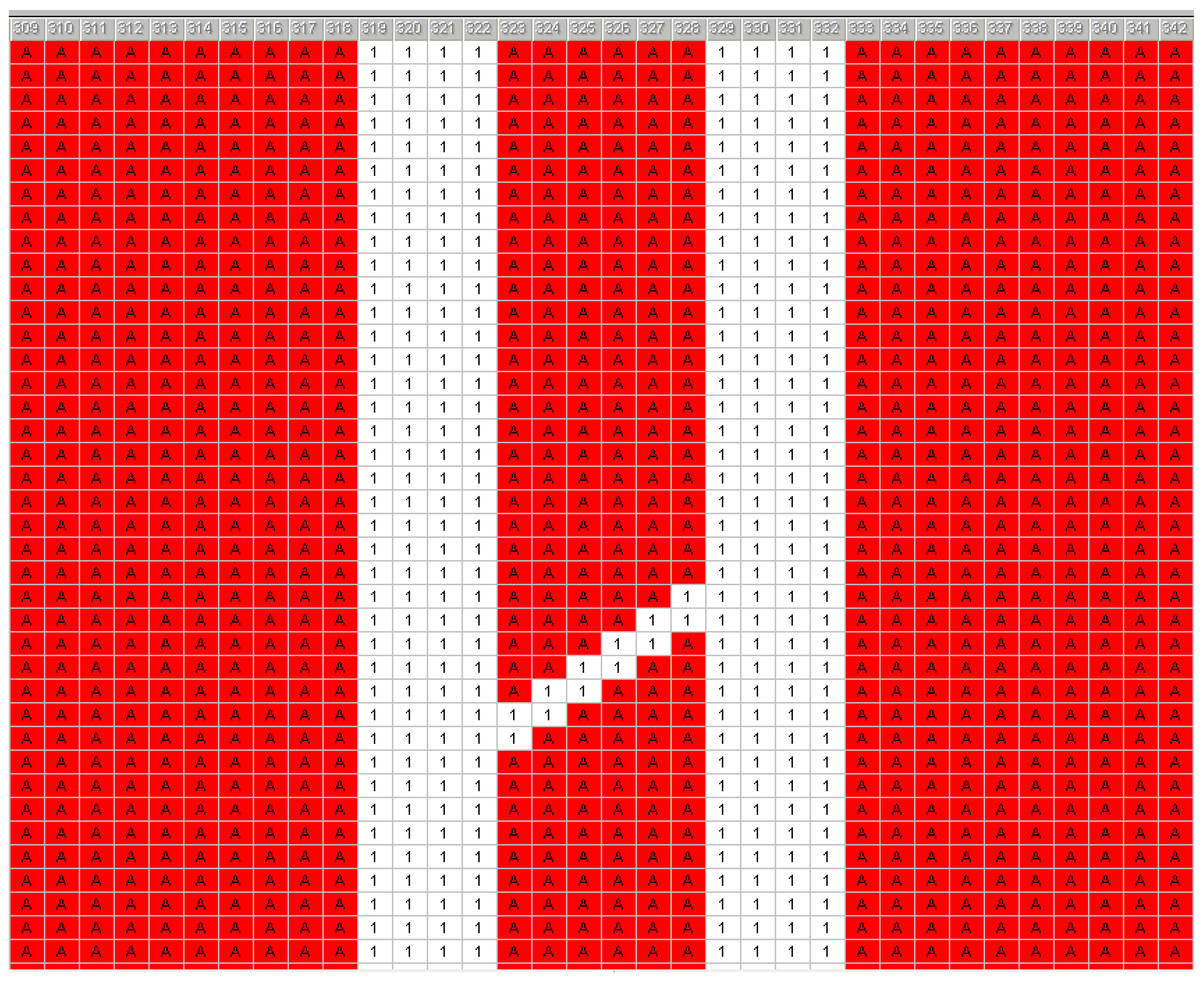
Figure 1 shows the top part of the Lamodel grid used. It is critical to note that all the excavations occupy the section from grid location 319 to 322 on the
X-axis to ensure a comprehensive understanding of the presented Lamodel results. Notably, the grid numbers for the
Y-axis are numbered from the top downwards. For all the plots, distance along the cross-section is in meters (m). The letter ‘A’ in the Lamodel grid is used to represent the material type and its corresponding material properties. Different letters are used for different materials in order to allocate the different material properties to the different material types. In this study, only one material type was used, hence the use of the letter ‘A’ (material type 1) throughout the Lamodel grid.
Lamodel Plan Views of Results
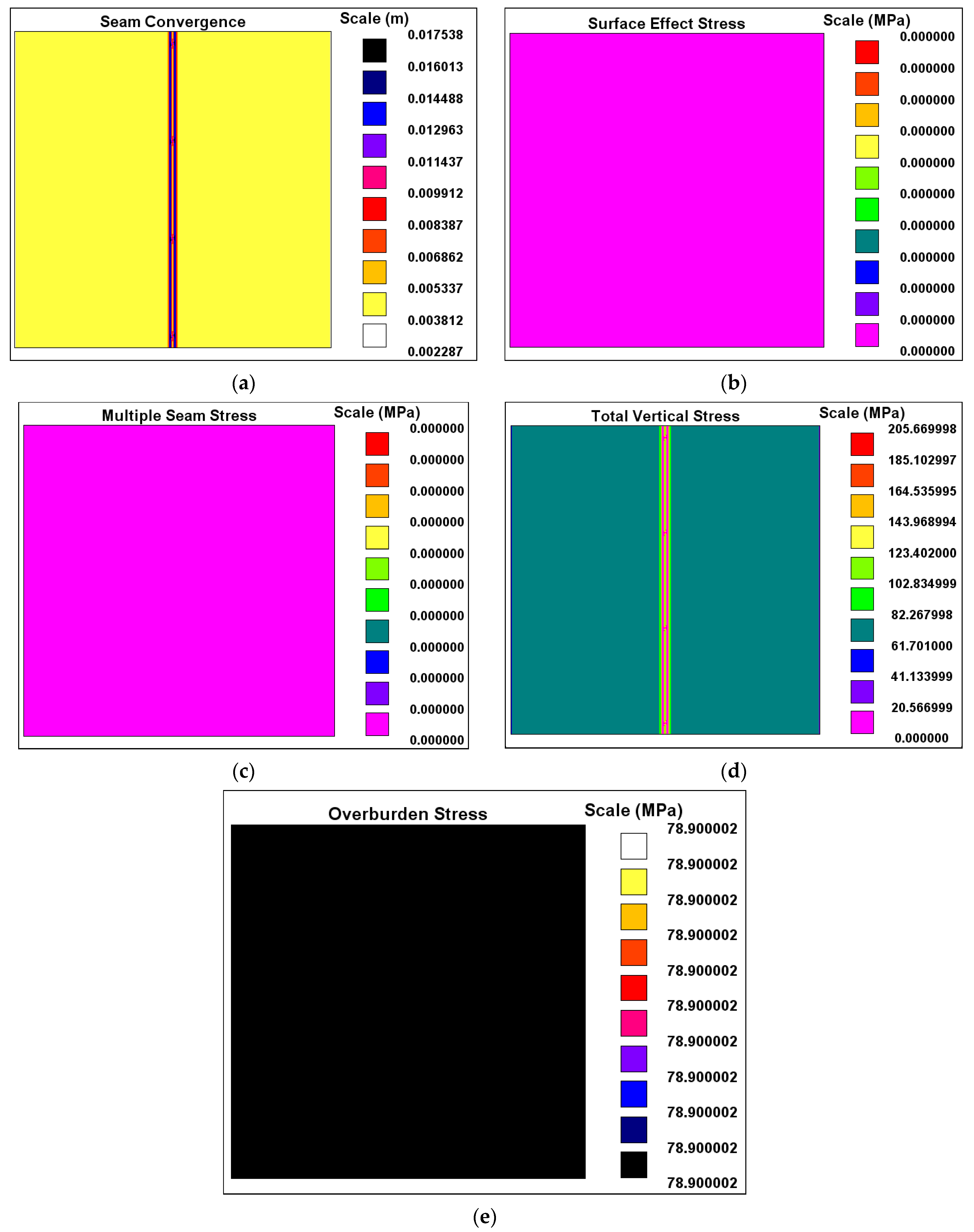
From the modelling results, it can be interpreted that seam convergence is significant in all the areas of open excavations. Seam convergence is most significant in the tunnels since the planner surface opening (4 m) is higher than that of the interconnections (2 m), resulting in considerable overburden stress acting around the tunnels. A depth of 3000 m is quite large, resulting in the excavation experiencing no surface effect stress. Only one seam was used in the analysis; therefore, the multiple seam stress was found to be zero, as expected. The total vertical stress was highest along both the tunnels and the interconnections, because these areas are more susceptible to stress effects due to their openness. Given a material density of 2700 kg/m
3, gravitational acceleration of 9.81 m/s
2, and a depth of 3000 m, the vertical stress where the excavations were located was calculated to be 79.46 MPa. As expected, the model yielded almost the same result (78.9 MPa) in its determination of overburden stress. The results are depicted in
Figure 2.
Figure 2 presents different plan view results of different aspects under analysis for the study. The purpose of the plots is to give an overview of the distribution of the study parameters within the whole study area (650 m × 650 m grid). Different grid locations are then selected from the
Y-axis, parallel to the
X-axis, to assess the distribution of different sequences of excavations intersected by the grid lines. This is also done for the X-axis, parallel to the Y-axis. Notably, the surface effect stress was zero because deep excavations were the subject of analysis here. Additionally, because Lamodel has been used for unlaminated hardrock mass analysis, a single layer was used; therefore, a multiple seam stress of zero was recorded.
3. Lamodel Cross-Sectional Plots
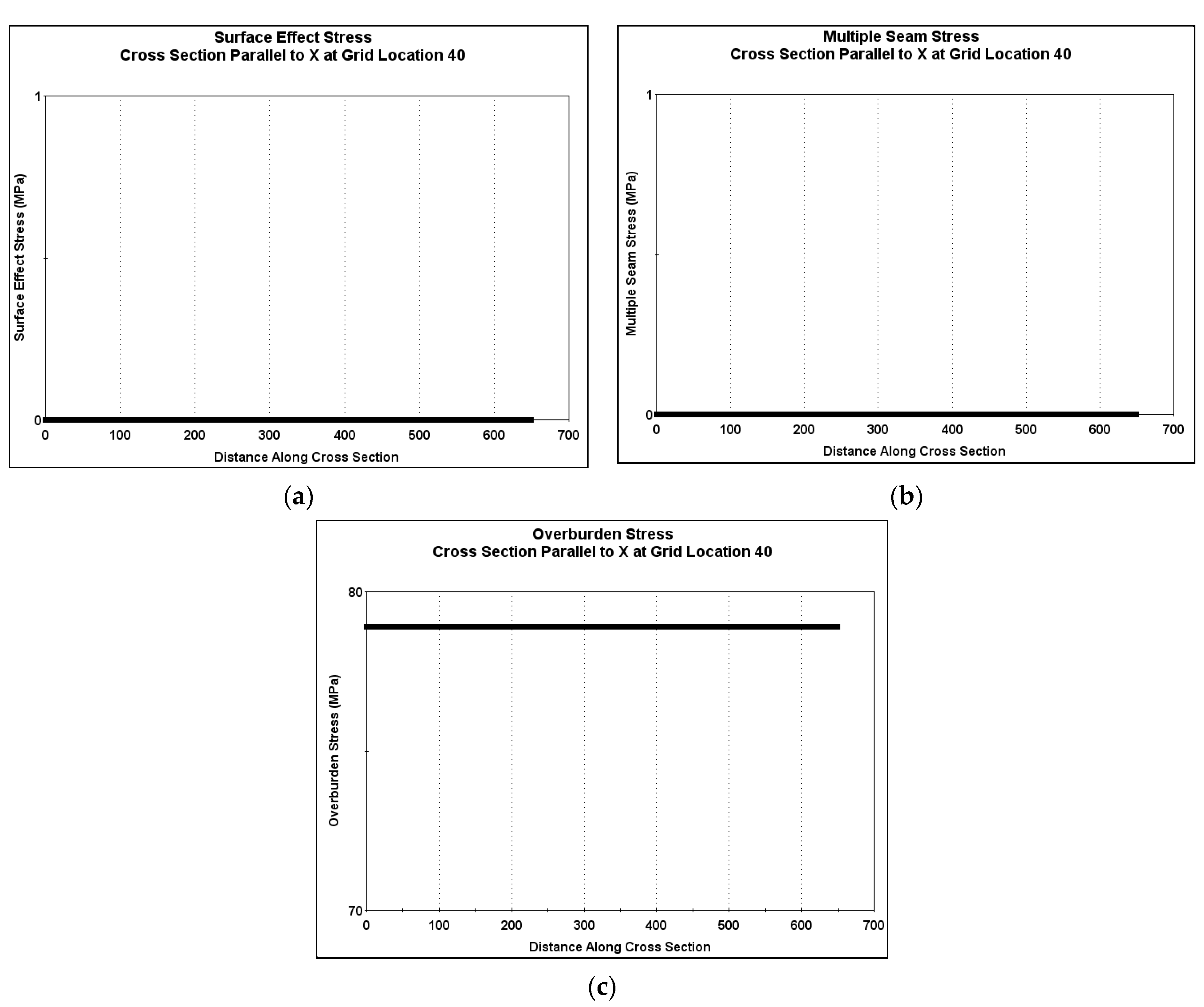
3.1. Subsection Surface Effect Stress, Multiple Seam Stress, and Overburden Stress
The cross-sections parallel to X or Y at any grid location for surface effect stress and multiple seam stress were the same. Both stress values were found to be zero along the cross-sections. This serves as a confirmation of the results obtained with coloured square plots. As expected from the coloured square plots, the overburden stress cross-sections parallel to X or Y at any grid location were confirmed to be 78.9 MPa.
Some results illustrating the above explanations are presented in
Figure 3. The overburden stress cross-section parallel to Y is presented in Figure 7a at X-axis grid location 302, representing the region at a distance sufficiently away from the excavations, not to be influenced by the excavations.
3.2. Seam Convergence and Total Vertical Stress Cross-Sectional Plots
3.2.1. Seam Convergence Cross-Sections Parallel to X at Selected Grid Locations
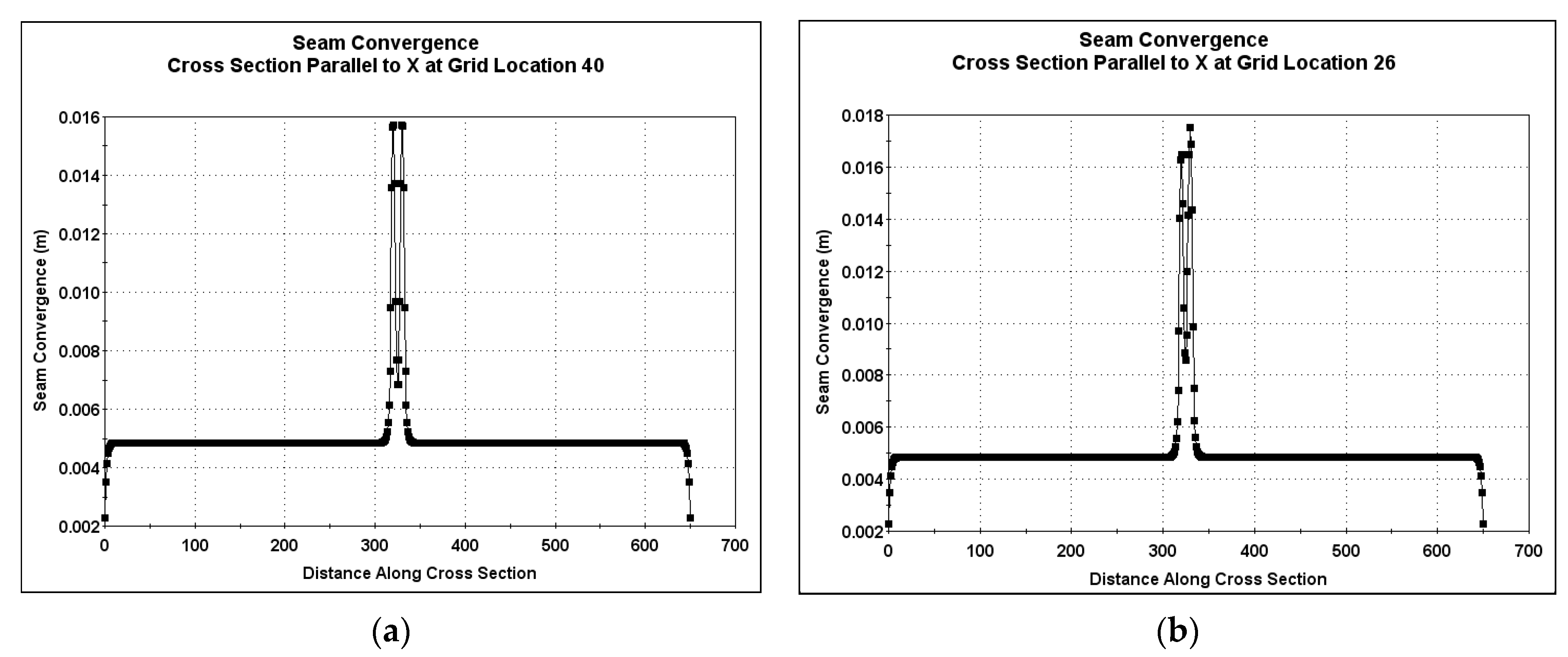
The seam convergence cross-sections for the scenario where the cross-section ran parallel to X at grid locations following the following sequence were the same: Whole Solid Rock → First Tunnel → Solid Pillar between Tunnels → Second Tunnel → Whole Solid Rock.
Some of the grid locations which followed this profile were 40, 130, 330, and 530. Grid location 40 has been taken for illustrative purposes, as shown in
Figure 4a. The cross-sections indicate that a low seam convergence of approximately 0.005 m was encountered in the solid rock, whereas there was a sharp rise to a seam convergence of 0.016 m in both tunnels. This was due to the stress concentration on the open tunnels compared with that of solid rock. Additionally, the seam convergence cross-sections for the scenario where the cross-section runs parallel to X at grid locations along the following sequence were the same: Whole Solid Rock→ First Tunnel → Solid Rock → Interconnection → Solid Rock → Second Tunnel → Whole Solid Rock.
Some of the grid locations which follow this profile are 26, 226, 426, and 626.
The latter sequence was illustrated using grid location 26, as shown in
Figure 4b. As explained previously, the seam convergence remained the same at about 0.005 m in the whole solid rock section and sharply rose to above 0.016 m in the tunnel and interconnection openings due to a concentration of stress in these areas.
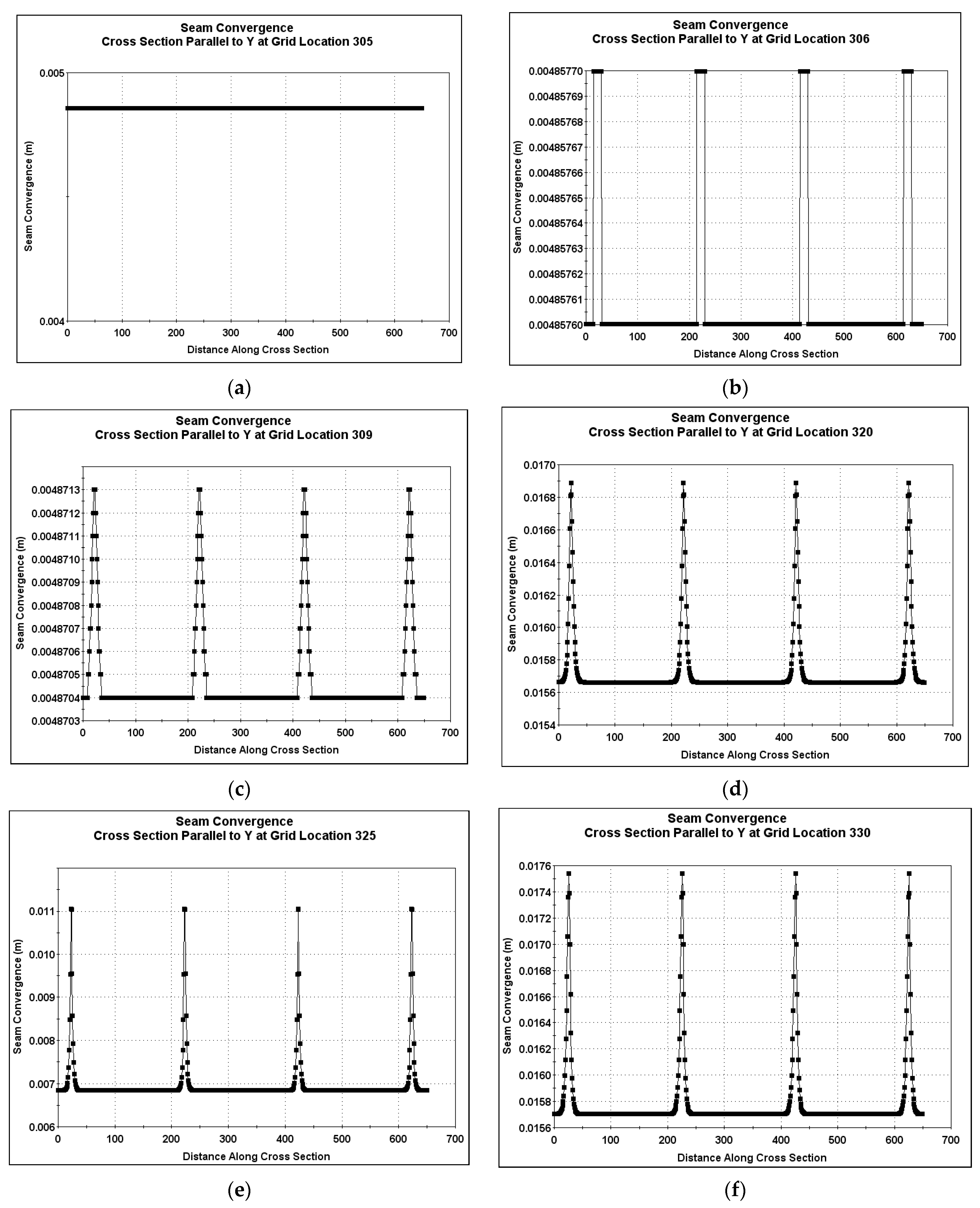
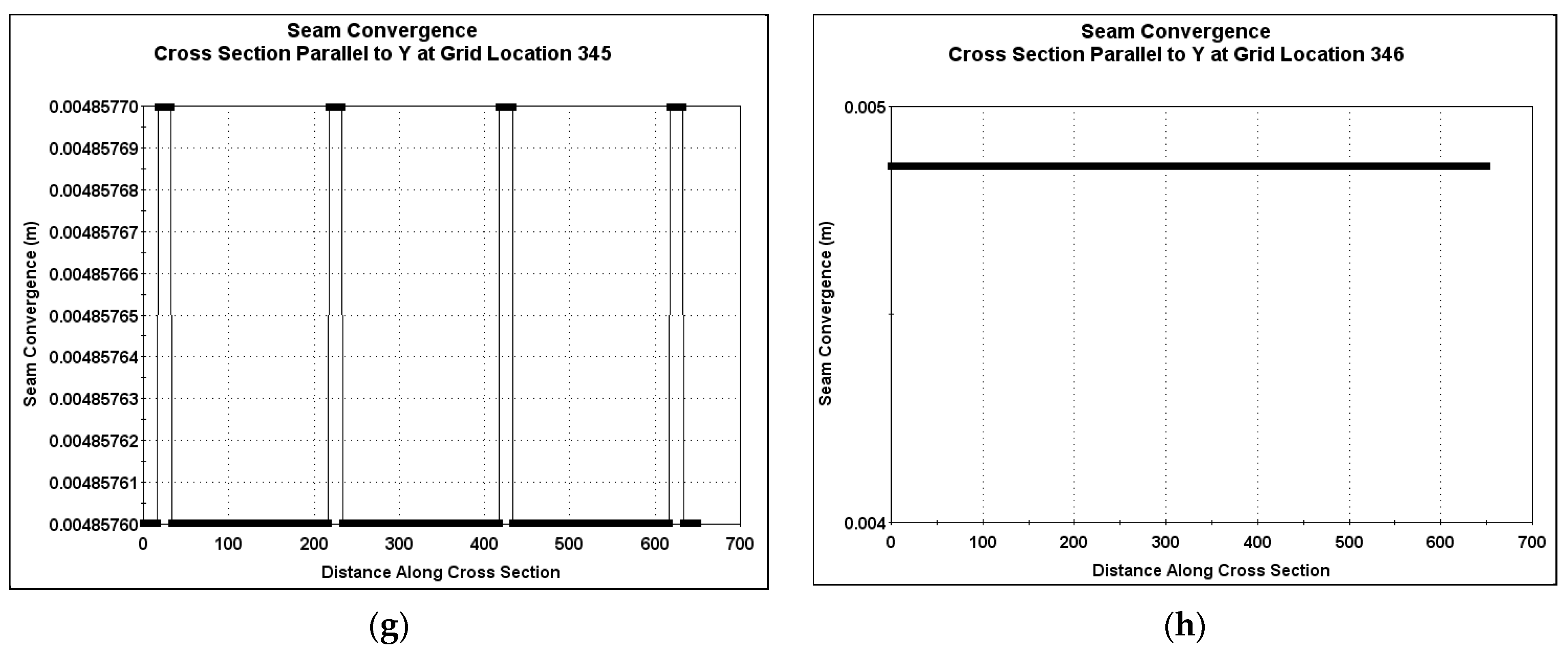
3.2.2. Seam Convergence Cross-Sections Parallel to Y at Selected Grid Locations
As shown in
Figure 1, all the excavations occupied grid locations 319 to 322 on the
X axis, meaning there was total solid rock before grid location 319 and after grid location 322. The seam convergence cross-sections parallel to Y showed that the effects of the interconnections were felt in the solid rock from grid location 305 up to grid location 346. Running through each cross-section, there was a sharp rise in convergence at all positions where there was an influence of interconnections. Interconnections are points of weakness; thus, stress at these zones caused the sharp rises in seam convergence. The results of the cross-sectional plots are shown in
Figure 5.
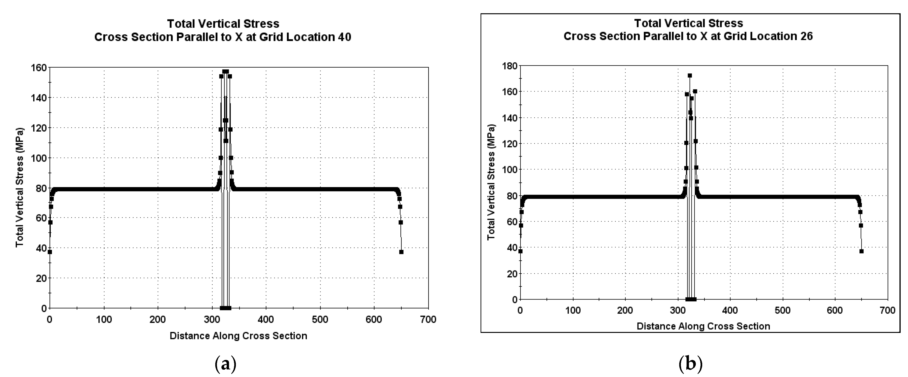
3.3. Total Vertical Stress Cross-Sections Parallel to X at Selected Grid Locations
The total vertical stress cross-sections for the scenario where the cross-section runs parallel to X at grid locations following the following sequence are the same: Whole Solid Rock → First Tunnel → Solid Pillar between Tunnels → Second Tunnel → Whole Solid Rock.
Some of the grid locations which follow this profile are 40, 130, 330, and 530. Grid location 40 has been taken for illustrative purposes, as shown in
Figure 6a. It can be seen from the cross-section that a total vertical stress of approximately 80 MPa was encountered in the solid rock while there was a sharp rise to a total vertical stress of 160 MPa in both tunnels. This is due to stress concentration on the open tunnels compared with the solid rock. Additionally, the total vertical stress cross-sections for the scenario where the cross-section runs parallel to X at grid locations following the following sequence are the same: Whole Solid Rock → First Tunnel → Solid Rock → Interconnection → Solid Rock → Second Tunnel → Whole Solid Rock.
This sequence is illustrated using grid location 26. As explained before, the total vertical stresses remained the same at approximately 80 MPa in the whole solid rock potion and sharply rose to above 160 MPa in the tunnels and to approximately 165 MPa in the interconnections. The lower surface of the interconnections contributes to a higher stress level acting on them compared with the tunnel openings. Some of the grid locations that follow this profile are 26, 226, 426, and 626.
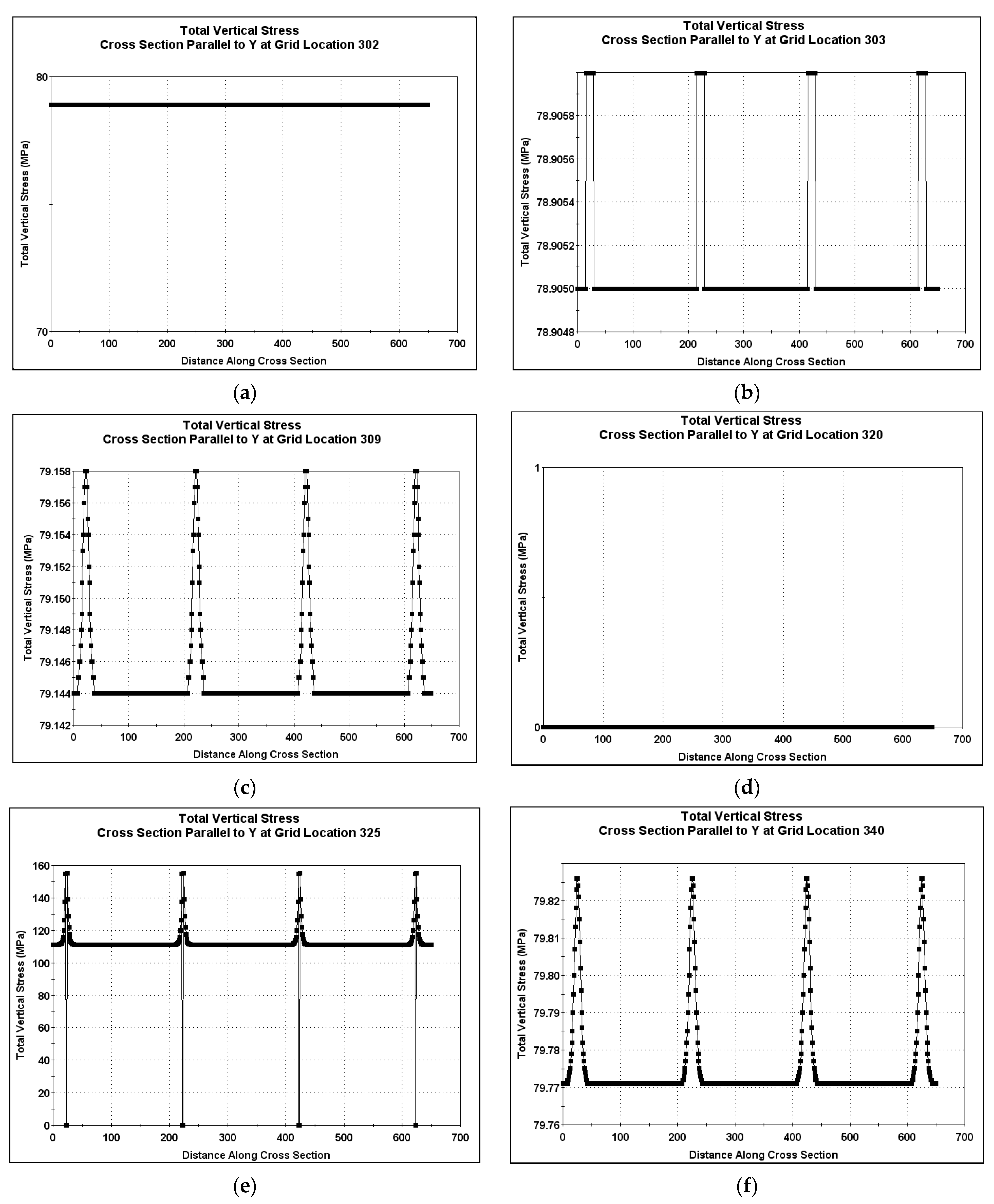
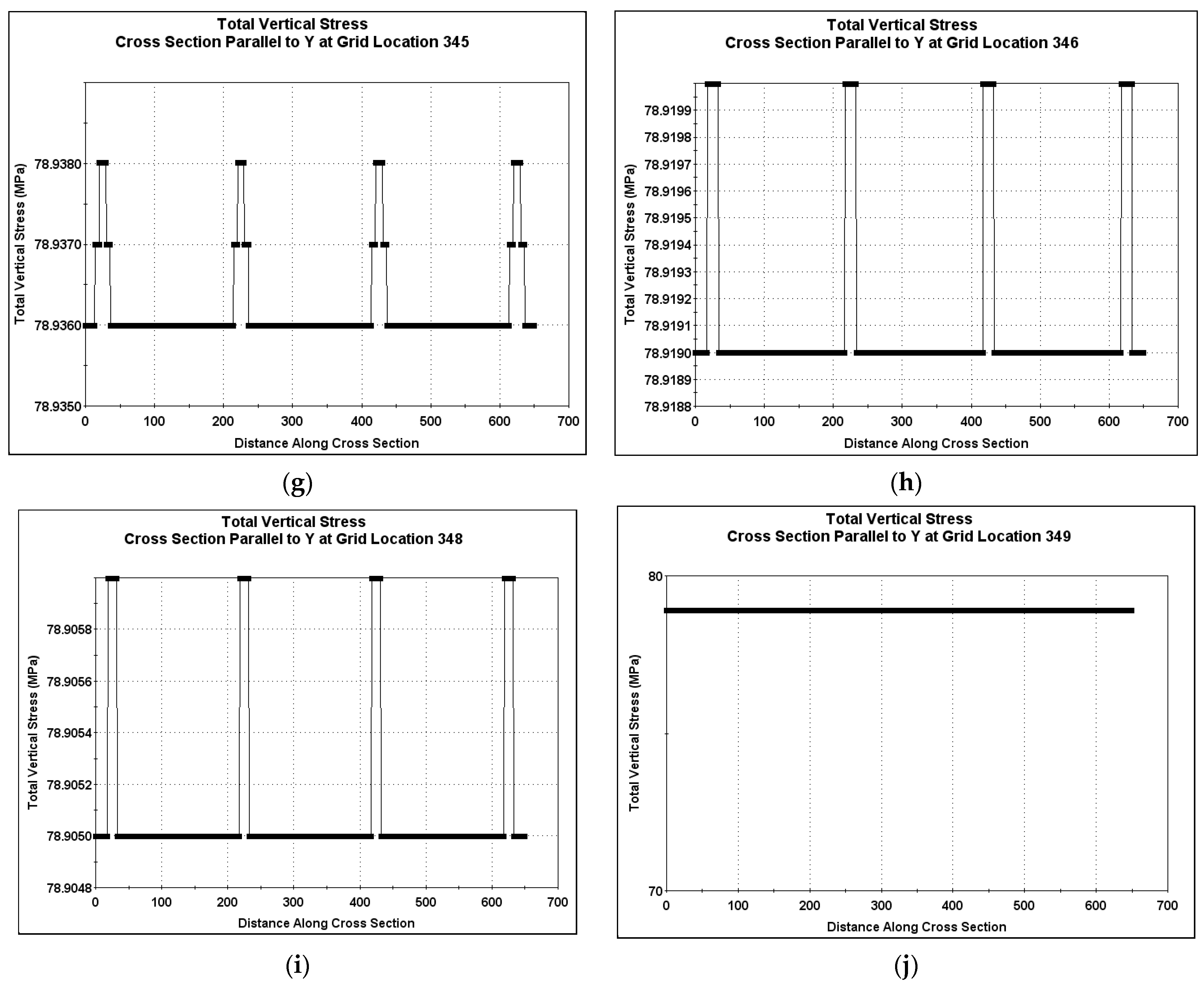
3.4. Total Vertical Stress Cross-Sections Parallel to Y at Selected Grid Locations
As shown in
Figure 1, all the excavations occupied grid locations 319 to 322 on the
X axis, meaning that there was total solid rock before grid location 319 and after grid location 322. The total vertical stress cross-sections parallel to Y show that the effects of the interconnections were felt into the solid rock from grid location 302 up to grid location 349. Running through each cross-section, there was a sharp rise in total vertical stress at all positions where there was influence of interconnection. Interconnections are points of weakness; therefore, stress at these zones caused the sharp rises in total vertical stress. The results of the cross-sectional plots are shown in
Figure 7.
The total vertical stress was zero at all open locations along any cross-section parallel to Y.
To facilitate the understanding of the results presented in
Figure 7, remember that the Lamodel grid used for the overall analysis of the rock engineering problem was 650 m (
X-axis) x 650 m (
Y-axis). The grid numbers for the
X-axis are numbered from 1 to 650 (each grid is 1 m) from left to right of the Lamodel grid (
Figure 1), while the grid numbers for the
Y-axis are numbered from 1 to 650 (each grid is 1 m) from the top to the bottom of the Lamodel grid (
Figure 1). For all the plots, the distance along the cross-section is in meters (m).
4. Fishnet Results
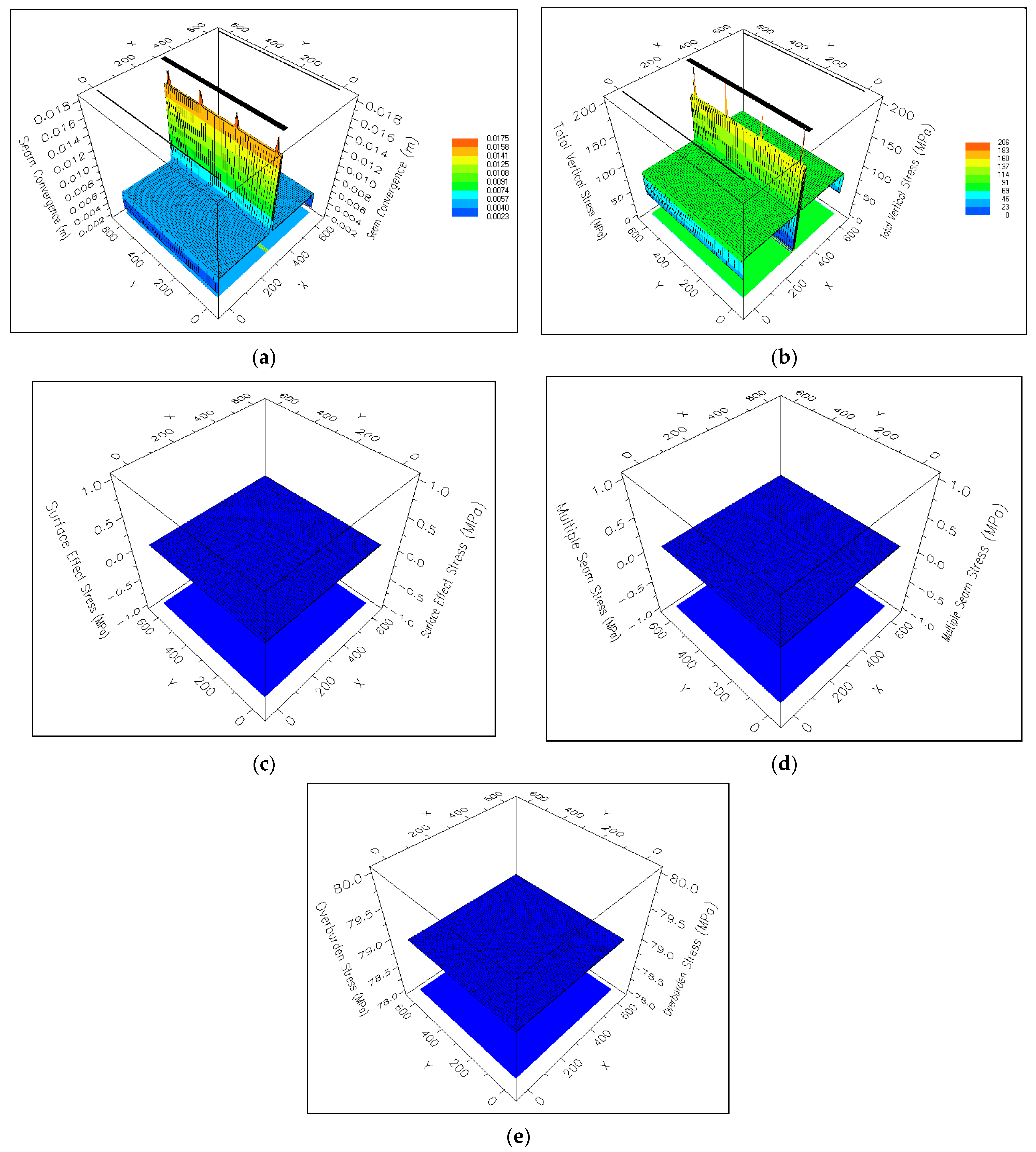
The results of the cross-sectional plots of the different variables were clearly visualised in 3D using the fishnet function of Lamodel. The fishnet function is a powerful tool in Lamodel which enables simple visualisation of the overall results of any variable. The fishnet results show that the seam convergence in all solid rock locations was constant at approximately 0.005 m, although it spiked to approximately 0.016 m in the tunnels due to the influence of the stress concentration. As expected, the total vertical stresses were zero in all the openings, i.e., the tunnels and the interconnections. The total vertical stress for the solid rock locations was approximately 79 MPa, which sharply rose to approximately 160 MPa in the tunnel openings and distinctly rose above 160 MPa at each of the connections, as shown by the four spikes in fishnet for total vertical stress. The fact that surface effect stresses and multiple seam stresses were zero where the excavations were located was also emphasised by fishnet. Both fishnet diagrams for these two variables exhibited stress values of zero. The overburden stress was calculated to be around 79 MPa, as depicted in the coloured square plots and the cross-sectional plots; likewise, the fishnet diagram for the overburden stress verifies this stress level. Fishnet results are presented in
Figure 8.
Figure 8c–e are single-coloured and presented in 3D to highlight the strengths and different analysis options available in the Fishnet function of Lamodel software.
5. Examine 2D
Examine 2D is quick and simple-to-use modelling software which enables parametric studies and preliminary designs of a problem before modelling it with sophisticated software. Examine 2D is two-dimensional and assumes that the rock to be modelled is elastic; it also utilises plain strain analysis whereby the strain in the out-of-plane direction of an excavation is assumed to be zero. One can easily define the excavation dimensions and also label any variable magnitude in Examine 2D. As a result of its simplicity, it is a good initial teaching tool for geotechnical stress analysis.
As with all other modelling software programs, awareness of the strengths and the limitations of Examine 2D is critical for the reasonable interpretation of the results. Due to its plane strain assumptions, Examine 2D can only model homogeneous, isotropic/transversely isotropic, or linearly elastic rock masses. It can only model and display the elastic component of displacements. Some of the problems which cannot be modelled using Examine 2D are multiple material plasticity/yielding/progressive failure, support, staging, joints, and pore pressure.
5.1. Model Building
The project settings were input as per the problem requirements. Two failure criteria were used: the Mohr–Coulomb failure criterion and the Hoek–Brown failure criterion. Before discussing the results of the modelling, it is imperative to discuss the rock failure criteria used.
5.1.1. Mohr–Coulomb Failure Criterion
This criterion serves to describe the response to shear stress and normal stress by materials. This criterion was used in the analysis due to its ability to predict failure to a high degree of accuracy (Griffiths [
11]; Bai and Wierzbicki [
12]; Hackston and Rutter [
13]). It is also a powerful tool for determining the cohesion and friction angle of rocks, which are important parameters to determine for the reliable prediction and design of structures in rock masses. However, the Mohr–Coulomb failure criterion has its own drawbacks, as given below (Stacey [
14]; Saeidi et al. [
15]; Tian and Zheng [
16]; Wu et al. [
17]):
It implies that a major shear fracture occurs at peak strength.
It implies a direction of shear failure which often does not agree with observations, particularly in brittle rock.
It is linear, and peak strength envelopes determined experimentally are usually non-linear.
It assumes that cohesion and friction act fully in unison.
The criterion is likely to give incorrect results if the failure mechanism is not shear.
The criterion ignores σ2 and only uses σ1 and σ3 but σ2 has influence on the failure of rocks.
The Mohr–Coulomb failure criterion can be represented by Equation (1).
where τ is shear stress along the shear plane at failure, σ
n is normal stress acting on the shear plane, c is the initial cohesive strength, and ϕ is the angle of internal friction.
This formula can also be presented as in Equation (2).
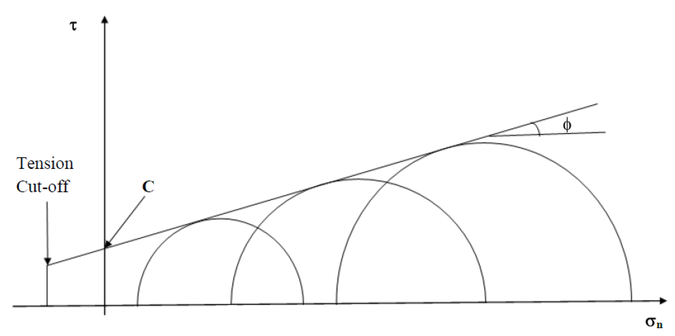
The orientation of the predicted failure plane is given as (45 + ϕ/2) degrees, measured in the σ1–σ3 plane from the σ3 axis.
A plot of Mohr circles in shear stress against normal stress space can be used to determine the cohesion and friction angle by plotting a Mohr envelope which is tangential to the Mohr circles. The angle of friction can be extrapolated from the gradient of the Mohr envelope, while the cohesion is the vertical intercept of the Mohr envelope. The Mohr envelope is illustrated by a diagram illustrated by Zvarivadza [
18], as shown in
Figure 9.
In addition, methods such as the Apex point plot and the plot of σ1 against σ3 can be used to determine cohesion and the angle of friction; however, these are beyond the scope of this discussion.
5.1.2. Hoek–Brown Failure Criterion
Basically, the results of modelling using this failure criterion are almost the same as those numerical modelling results obtained using Mohr–Coulomb failure criterion. This is because most of the formulation assumptions of the two criteria are the same. Similarly to the Mohr–Coulomb failure criteria, the Hoek–Brown failure criterion is used to describe the response to shear stress and normal stress by materials. It was used in modelling the given problem as it served to verify the results from the numerical modelling using Mohr–Coulomb failure criterion. Any considerable difference would definitely mean a modelling error somewhere in the process.
The Hoek–Brown failure criterion is represented by Equation (3).
where m
b is the Hoek–Brown constant,
m, for the rock mass, s and a are constants which depend on the rock mass characteristics, and σ
ci is the UCS of the intact rock.
For intact rock, the Hoek–Brown equation reduces to Equation (4).
where mi is the Hoek–Brown constant for the intact rock.
The drawbacks of the Hoek–Brown failure criterion are similar to the Mohr–Coulomb failure criterion since it is also shear-based. Stacey [
14] mentioned that the Hoek–Brown failure criterion applies to the “central” range of rock masses, which is well-jointed rock mass in which the joints control behaviour rather than the rock material or individual significant planes of weakness.
5.1.3. Extension Strain Failure Criterion
This is another failure criterion which can be used to model failure of rocks. However, it is not in built in Examine 2D and could not be used for this study. As a simple but robust tool for introducing rock engineers to numerical modelling, Examine 2D only incorporates Mohr–Coulomb and the Hoek—Brown failure criteria in its formulation. The Extension Strain failure criterion works very well for predicting failure in brittle rocks and estimating the spalling of underground cavities in circumstances where rock failure occurs under stress levels not considered to be critical. In intact rock, the criterion also works very well. Stacey [
19] described the criterion as follows: ‘Fracture of brittle rock will initiate when the total extension strain in the rock exceeds a critical value which is characteristic of that rock type.’ The criterion can be expressed using a mathematical expression as in Equation (5).
where e
c is the critical value of the extension strain. The stress–strain relationship which can be used to calculate the minimum principal strain is given in Equation (6).
where σ
1, σ
2, and σ
3 are the principal stresses, E is the modulus of elasticity, and ν is Poisson’s ratio. Stacey [
19] pointed out that an extension strain occurs when ν (σ
1 + σ
2) > σ
3.
The extension strain failure criterion is advantageous because it automatically accommodates all the three-dimensional stresses. It is also in agreement with most of the fracturing observed in brittle rock failures. Although researchers such as Martin [
20], Martin et al. [
21], Wesseloo [
22], Diederichs [
23], and Eberhardt et al. [
24] agree with the use of this criterion in estimating the spalling of underground cavities, Kuijpers [
25] pointed out that the criterion fails to address the physics involved in the formation of fractures in compressive stress environments.
5.2. Hoek–Brown and Mohr–Coulomb Model Results Considering Fundamentals of the Mechanics
The Hoek–Brown failure criterion is an empirical relationship based on the concepts of rock mass strength and its response to high-stress levels. It integrates both intact rock strength and the effect of structural discontinuities (such as joints, faults, and bedding planes) on rock mass behaviour. This model considers the presence of geological structures and their influence on the overall strength of rock masses. The Hoek–Brown model uses several parameters to define rock mass strength, including the Geological Strength Index (GSI), the Hoek–Brown constant (mi), and the uniaxial compressive strength (σc). These parameters encapsulate the intact rock strength and the influence of structural discontinuities on rock mass behaviour. The Hoek–Brown model is widely used in tunnelling and underground excavations, where rock masses may have complex structures and are affected by stress redistribution and geological factors.
The Mohr–Coulomb linear failure criterion relates normal and shear stresses to the strength of materials. It is used to define the strength of intact rock materials rather than the overall behaviour of rock masses, focusing more on failure conditions in intact rock materials. The model utilises cohesion (c) and internal friction angles (ϕ) to describe the strength of intact rock materials. Cohesion represents the strength of the material when no shear stress is applied, while the internal friction angle represents the resistance to sliding when stress is applied. It is commonly used in geotechnical engineering and civil engineering for analysing the stability of slopes, foundations, and rock masses subjected to surface loading.
The choice between Hoek–Brown and Mohr–Coulomb models depends on the context and the goal of the analysis. For analysing rock mass behaviour and stability in the presence of discontinuities, the Hoek–Brown model is often preferred. For assessing the stability of intact rock materials in engineering applications, the Mohr–Coulomb model is commonly utilised. Both models offer valuable insights into rock mechanics, each with their own unique approach and application scope.
6. Analysis of the Examine 2D Results
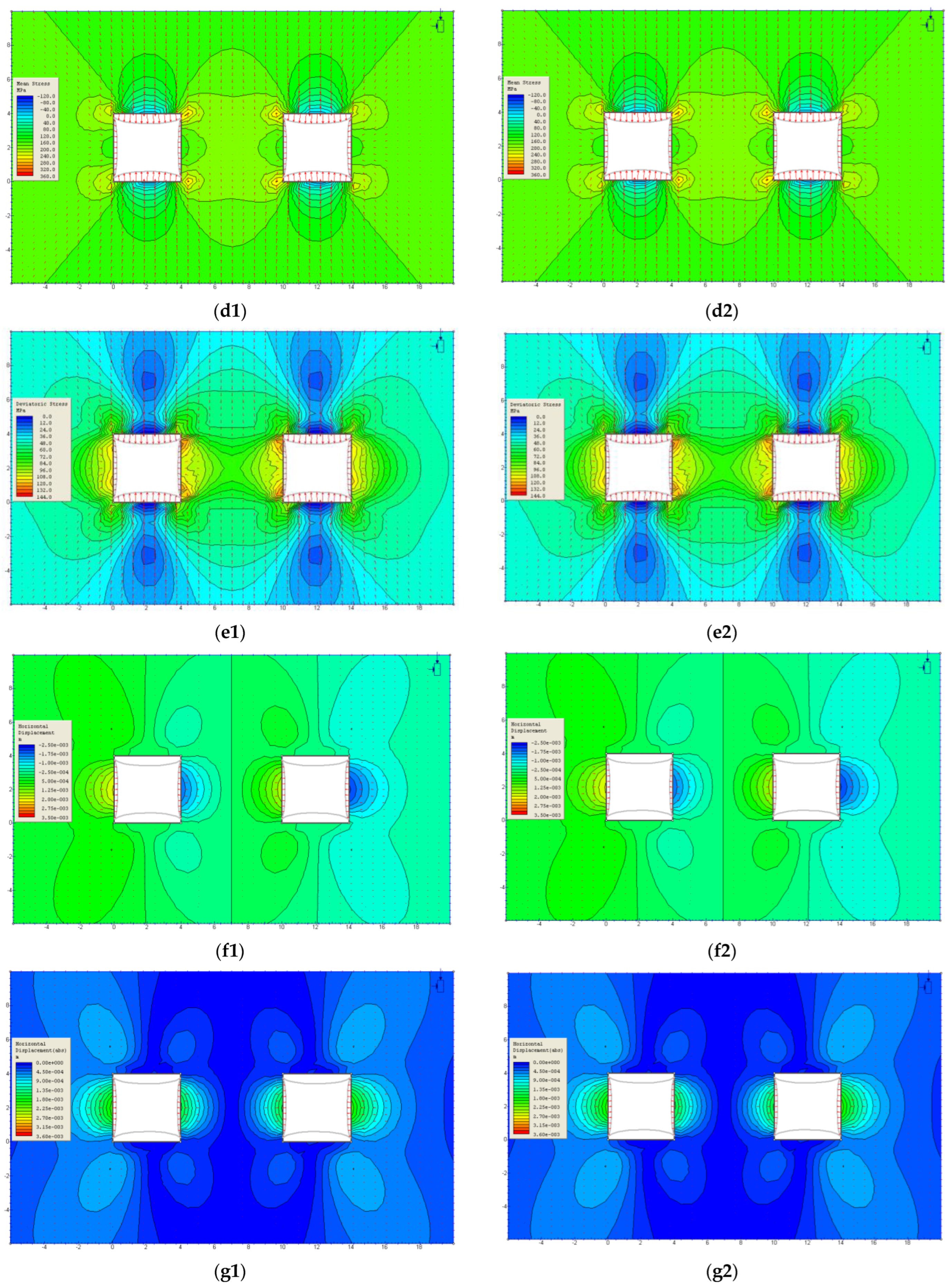
The Examine 2D results using Mohr–Coulomb and Hoek–Brown failure criteria are almost the same and one can hardly see the difference. It is important to note that the excavation cross-sections were used in Examine 2D, unlike in Lamodel where we used the plan view of the excavations. The modelling schemes of Lamodel and Examine 2D are expressed separately in this paper. As noted, Examine 2D could not model the interconnections, and the simulation schemes were obviously different. In the Examine 2D results shown in
Figure 10, all the results display deformed boundaries, deformation vectors, and filled contour lines. The results obtained from both failure criteria are presented here to illustrate that, in some rock engineering applications, either the Mohr–Coulomb or the Hoek–Brown failure criterion can be used for analysis without obtaining significant differences in the results. The full scatter plots of the domains analysed are presented to capture, as an overview, the complete picture of the distribution of the different rock engineering parameters under analysis. While queries could be plotted at any angle around the excavation, this would be insufficient to capture a complete picture of the distributions of the parameter under analysis.
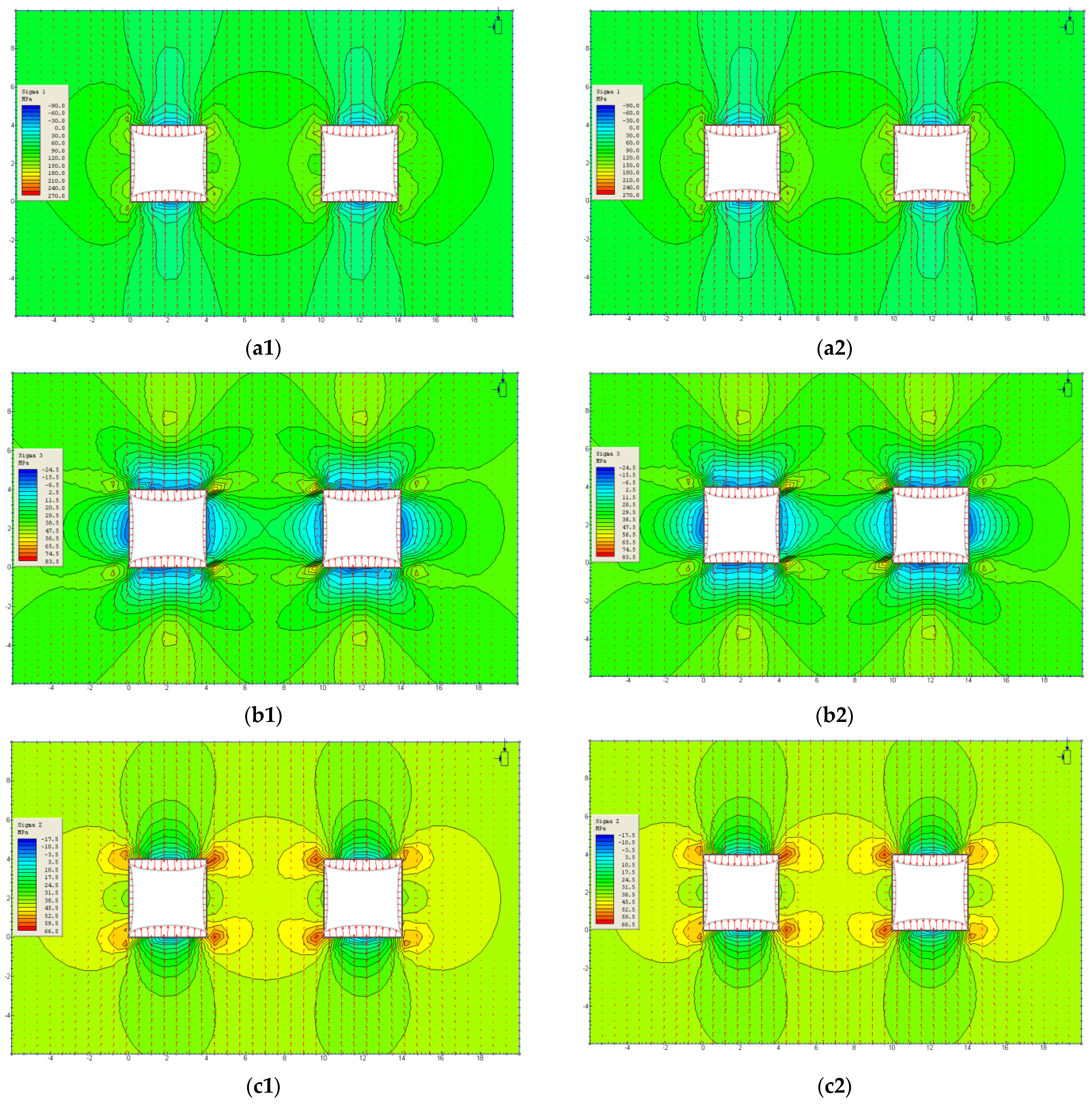
6.1. σ1 Stress Distributions
As shown in
Figure 10a, the σ
1 stresses were almost 0 MPa at both the top part and the bottom part of the excavations. The σ
1 stress levels increased as the distance away from the top and bottom edges of the excavations increased. This is a result of the little influence of total vertical stress on these edges, as shown in the Lamodel results.
6.2. σ3 Stress Distributions
As shown in
Figure 10b, σ
3 stresses were low, at approximately −15 MPa, at all the regions immediately after the excavation and increased to a maximum of 2.5 MPa at regions within the influence of the excavations. This is because σ
3, being the minimum stress, did not exert much stress around the excavations. Notably, stress interactions at internal corners directly opposite from each other caused a spike in stress to 65.5 MPa.
6.3. σz Stress Distributions
As shown in
Figure 10c, minimum stresses of 3.5 MPa were observed at both the immediate top and bottom of the excavations. The internal corners of both excavations experienced stresses of up to 59.5 MPa due to the superposition of stress fields from the corners. The external corners experienced approximately 52.5 MPa stress, although this was not highly concentrated because there were no stress field interactions.
6.4. P Mean Stress Distributions
Stresses of 0 MPa were experienced at the top and bottom of the excavations due to the nil influence of total vertical stress, as shown in
Figure 10d. Average stress values of 280 MPa was recorded at all corners of the excavations, although these were highly concentrated in the internal corners due to stress field intersections. The external corners were independent from these sorts of interactions.
6.5. Q Deviatoric Stress Distributions
According to Angelier [
26], deviatoric stresses have particularly important applications in the derivation of stress orientations and magnitudes from fault slip data.
Figure 10e shows that the vertical deviatoric stresses were approximately 0 MPa, whereas the horizontal stresses were as high as 120 MPa at the regions immediately next to the excavation edge, and they decreased outwards. This is because the influence of horizontal deviatoric stress decreases as the distance away from an opening edge increases.
6.6. Horizontal Displacements
Figure 10f shows horizontal displacements but does not totally ignore some vertical displacements. It can be seen that the horizontal displacement at the right side of each cross-section is negative at around −1.75 × 10
−0.03 m at the region immediately next to the excavation edge and increases to −1.00 × 10
−0.03 m at the furthest region within the influence of the excavation. Horizontal displacement in the right–left direction of each excavation was positive, and reached a high of 2.00 × 10
−0.03 m. This was as a result of sign conventions for displacement analysis.
6.7. Absolute Horizontal Displacements
Absolute horizontal displacement indicated the complete horizontal displacements around the excavations without factoring in any vertical displacements. Absolute horizontal displacements were only witnessed at the vertical edges of the excavations and were found to reach a high of 2.25 × 10
−0.03 m at regions immediately next to the vertical edges of each excavation. The displacements decreased to approximately 9.00 × 10
−0.04 m at the furthest region within the area of influence of the excavations, as shown in
Figure 10g.
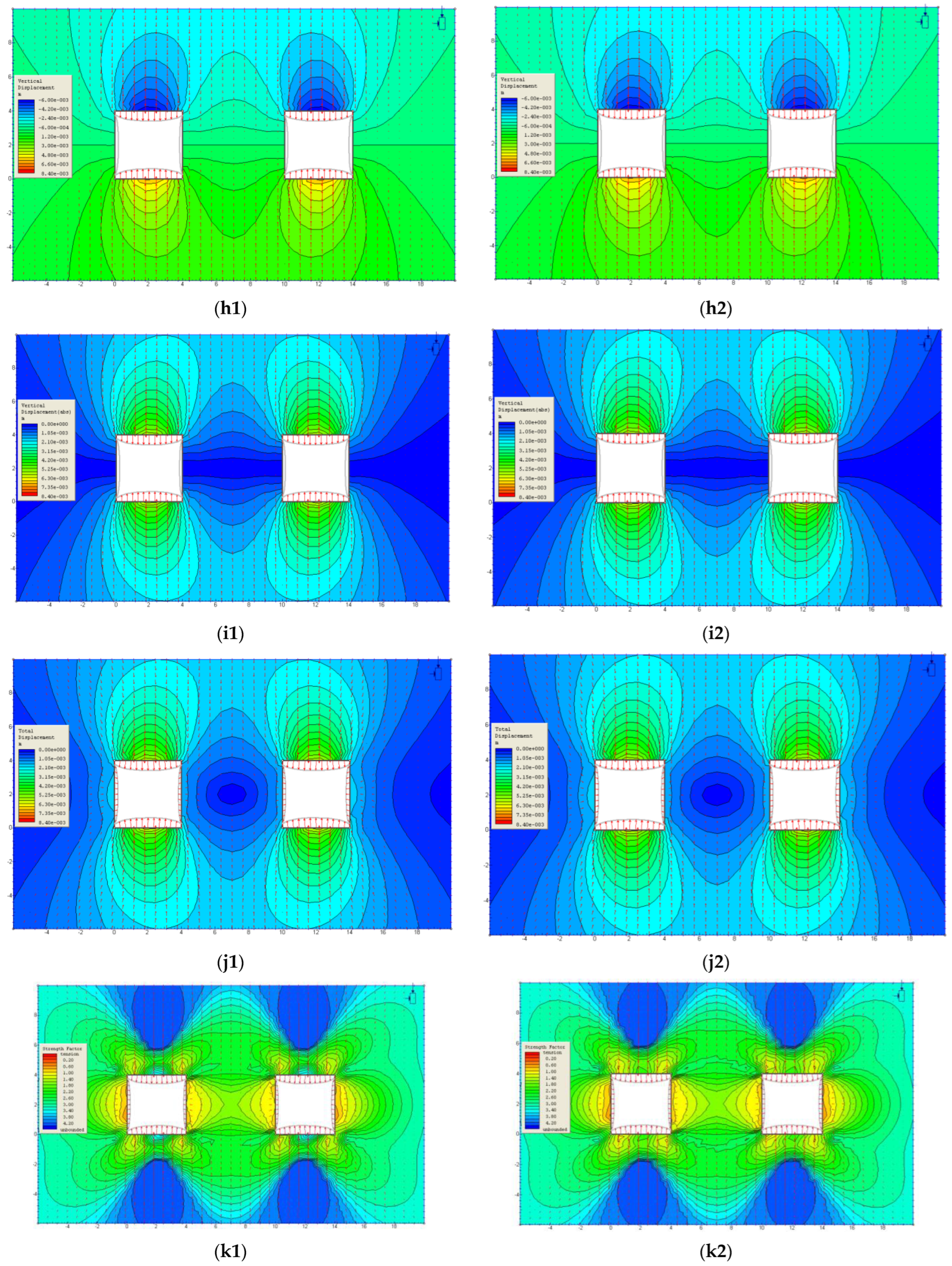
6.8. Vertical Displacements
The upper parts of the excavations experienced negative displacement of approximately −6.00 × 10
−0.03 at the region directly next to the top edges. This increased to approximately −2.40 × 10
−0.03 at the furthest region within the influence of the excavations. The lower parts of the excavations exhibited positive displacement of approximately 4.80 × 10
−0.03 m and decreased to approximately 1.20 × 10
−0.03 m, as shown in
Figure 10h. The stretching effect was a result of pressure release at the bottom of the tunnel, leading to tunnel floor swelling.
6.9. Absolute Vertical Displacements
Absolute vertical displacement represents the complete vertical displacements on the top part and the bottom part of the excavations after the horizontal displacements are ignored.
Figure 10i shows that when focusing on the absolute vertical displacements, the horizontal displacements were held at zero. The vertical displacements reached a high of 5.25 × 10
−0.03 m in solid rock regions just next to the top and bottom edges of both excavations. This decreased to a minimum of 2.10 × 10
−0.03 m at the furthest outer regions within the influence of the excavations. The reason for this trend is that absolute vertical displacement effectively acted vertically on these portions and the effect lessened as the distance away increased.
6.10. Total Displacements
Figure 10j plots the resultant effects of horizontal and vertical displacements. The results of the discussed absolute horizontal displacements are as shown in the vertical sides of the excavations. The results of the discussed absolute vertical displacements are also displayed on the top and bottom parts of the excavations.
6.11. Strength Factor
The strength factor represents the ratio of material strength to induced stress at any point. If this value is less than 1, it shows that the material will fail under the given stress conditions.
Figure 10k illustrates that the strength factor at the excavation corners was approximately 0.6; thus, failure will occur at these corners under the prevailing stress regime. The regions immediately next to the two outer vertical edges of the excavations exhibited a strength factor of about 0.6; therefore, failure will also occur here.
7. Comparison of Lamodel and Examine 2D
Examine 2D cannot model interconnections; however, Lamodel can. It is essential to note that the two modelling software programs complement each other. The results from Lamodel and Examine 2D can be combined to reveal a clearer picture of the problem at hand. It is not always that one serves to verify the other model’s results; they both contribute different results for different aspects of the problem. There are also other aspects of problems which can be independently modelled using each software package. In this study, Examine 2D provided numerical modelling results for the cross-section of a tunnel, assuming that the tunnel was in a plane strain state, and did not address what occurs ahead of the mining face. Lamodel resolves this shortcoming by being able to predict numerical modelling results of the situation ahead of the mining face. This is vitally important because stress build-up ahead of the mining face can result in catastrophic rock mechanics phenomena such as rockbursts, which have several implications on the safe, economic, and sustainable operation of the mine. In other rock engineering problems where different software programs can be used to model the same (single) aspect of the rock engineering problem, it is prudent to use only one of the techniques. The choice of software needs to be carefully considered to capture the mechanics and physics of the rock engineering challenge at hand, utilising findings from the literature, presented in this paper, to guide the choice.
8. Conclusions
It is vitally important for rock engineers to understand the influence of stress concentrations around deep mining excavations in order to design and implement appropriate stabilising measures. In endeavours to achieve this end, initial simple models can be used to gain understanding of the problem at hand. Complexity is gradually built into the models as many different aspects of the problem are accounted for. This study has demonstrated that Lamodel and Examine 2D, although simple and quick-to-use software, are robust modelling tools for diagnosing rock engineering challenges. The analysis shows that the Examine 2D results using the Mohr–Coulomb failure criterion were almost the same as the results obtained using the Hoek–Brown failure criterion. Parametric studies and other early stages of problem solving should be performed before applying more advanced software such as 3DEC or FLAC 3D to deal with the more complex parts of a problem. Numerical modelling is an important instrument for rock engineering, assisting in the design and prediction of failure in rock masses; however, one has to be aware of the assumptions, strengths, and weaknesses of the selected numerical modelling software if the interpretation of results is to be reliable. One has also to know what sort of results to expect from a model to be able to identify when the model has produced erroneous results. The element size greatly influences the accuracy and computational time in numerical modelling. The lower the element size, the higher the accuracy; however, the computational time also increases. A balance must be struck between computational time and accuracy, as this has cost implications.
Lamodel and Examine 2D complement each other in the numerical analysis of rock excavations. Lamodel captures the distribution of numerical modelling results ahead of the face, while Examine 2D presents the cross-sectional results and assumes that the excavation is in plane strain state. Stress concentrations ahead of the mining face pose significant mining challenges, such as potentially causing rockbursts. This study shows that the two software programs can be reasonably utilised for the preliminary investigation of rock excavations before more complex software can be used; this paves the way for detailed decision-making on which scenarios have to be investigated, with somewhat complex and time-consuming numerical model types. Different excavation sections were analysed using Lamodel, and extensive results are presented to illustrate the capability of the software, an aspect usually considered by practitioners when choosing what numerical modelling software to use in evaluations of rock engineering challenges. It is important to consider the fundamental mechanics of chosen constitutive models in numerical modelling. The Hoek–Brown and Mohr–Coulomb failure criteria are two distinct approaches used in rock mechanics for understanding rock behaviour under stress. The Hoek–Brown model accounts for the complexities of rock masses, considering intact rock strength and the impact of discontinuities such as joints and faults. It incorporates parameters such as GSI, mi, and uniaxial compressive strength to define rock mass strength, making it suitable for analysing tunnelling and excavations where complex structures and geological factors influence stability. Conversely, the Mohr–Coulomb criterion focuses on intact rock materials, defining strength through cohesion (c) and internal friction angle (ϕ) and can be extended to rock masses by deriving instantaneous internal friction angle and instantaneous cohesion in the field. It emphasises the resistance of rock materials to sliding under stress and is commonly used in geotechnical engineering for assessing deep mining excavations, foundations, and rock masses subject to high stress loading. The choice between Hoek–Brown and Mohr–Coulomb models depends on the analysis context. The Hoek–Brown model is preferred for assessing rock mass behaviour with discontinuities, while the Mohr–Coulomb model is better suited for evaluating the stability of intact rock materials in engineering applications. Both models offer distinct insights into rock mechanics, each tailored to specific contexts and analytical goals. The work presented in this paper could be extended to simulate the influence of destress drilling or destress blasting on the stability of deep mining excavations.


