1. Introduction
Modern climate changes are accompanied by a strong increase in global temperature, changes of precipitation patterns, and increases in the frequency and severity of extreme weather events. Most experts in climate change have associated these changes with an increase in the concentrations of greenhouse gases (GHG) in the atmosphere contributed mainly by various anthropogenic sources. Natural ecosystems actively influence the concentrations of GHGs (CO2, CH4, N2O, etc.) in the atmosphere. In particular, the natural ecosystems, on the one hand, release CO2 into the atmosphere through autotrophic and heterotrophic respiration, and on the other hand, they actively absorb CO2 from the atmosphere during photosynthesis. The reliable knowledge of GHG fluxes in natural ecosystems is obviously very important for the adequate projection of modern and future climate change.
A wide range of experimental methods is currently used to determine GHG fluxes between land surfaces and the atmosphere. The eddy covariance technique is the most widely used method in world practice for flux measurements; however, it has many limitations for its broader application [
1]. In particular, a significant limitation of the eddy covariance method is that it requires the homogeneity of vegetation canopies and surface topographies, which is rarely observed under natural conditions. Process-based mathematical models for GHG transfer can be very effective tools for describing the fluxes between heterogeneous land surfaces and the atmosphere.
The modern models of GHG transfer have different levels of complexity and use different approximations and simplifications for the description of vegetation properties [
2,
3,
4]. The most models describing the air flow distribution within the atmospheric surface layer are based on the system of the Navier–Stokes and continuity equations. In order to simplify the computational procedure, most existing models apply the Reynolds decomposition. Additional equations expressing unknown values through high-order moments are usually used to close the averaged system of equations [
5].
The simplest way to close a system of averaged equations is based on the Boussinesq conjecture, according to which a turbulent flux of some substance is assumed to be similar to molecular transport and proportional to a gradient of this substance. Presently, there are many models for describing the momentum transfer in the atmosphere (e.g., large eddy simulation (LES) models [
6]), and there are very few local models of mid-level complexity that allow us to operationally describe the GHG transfer within the atmospheric surface layer, taking into account the possible sinks and sources.
The main goal of this study was to develop a 3D model of the turbulent transfer of GHGs over a non-uniform land surface within the atmospheric surface layer and apply it to describe the spatial wind and CO2 flux distributions above the non-uniform forest peat-land “Staroselsky Moch” in the central part of European Russia.
2. Materials and Methods
2.1. System of Equations for Velocity Components and Turbulent Exchange Coefficient
For the wind velocity vector
, we use the Reynolds decomposition
to separate the average component
and the “fluctuating” component
with a zero average. In the used approximation, the air is considered to be incompressible. In the case of neutral atmospheric stratification, the average wind velocity
satisfies the following system of equations [
7]:
where
ρ is the average air density,
P is the pressure,
is the acceleration of gravity, and
and
are the specific forces of Coriolis and vegetation resistance, respectively.
The specific resistance force of vegetation can be parameterized as follows [
8]:
where
is a dimensionless coefficient of the vegetation resistance and
PLAD(
x,
y,
z) is the phytomass density, which includes both the foliage (
LAD) and non-photosynthetic (
SAD) elements of plants (branches and trunks):
PLAD =
LAD +
SAD.
In our model, we use the so-called “one-and-a-half” closure scheme and the Boussinesq hypothesis [
3,
9] to parameterize the turbulent fluxes
,
, and
as follows:
where
E is the turbulent kinetic energy (TKE) and
K is the turbulent exchange coefficient. The one-and-a-half order closure (or two equation closure) assumes that the coefficient
K is calculated using the TKE and its dissipation rate
(
), and that the functions
E and
satisfy the diffusion-reaction-advection type equations [
3,
9].
2.2. Initial and Boundary Conditions for the Dynamical Part of the Model
The system of Equation (1) is solved in a rectangular domain with some initial wind distribution, using the method of establishing. The initial and boundary conditions are consistent with a classical “one-dimensional” model describing turbulent conditions over a horizontally homogeneous surface, as follows:
where
α is the angle between the direction to the north and the average wind direction,
is the friction velocity,
is von Kármán constant, and
is the minimum value of the surface roughness layer within the modeling area. The upper boundary conditions are [
10]:
At the lower boundary of modeling domain, a velocity of zero is assumed. For the vertical component of wind velocity at the lateral boundaries, we use a zero Neumann condition. To set the lateral boundary conditions for the horizontal wind velocity components, we divide the lateral boundary into the “windward” and “leeward or free” parts, depending on the wind direction. At the input boundaries, the horizontal wind velocity is considered to be known, and at the leeward boundaries, we use a zero Neumann conditions. The initial and boundary conditions for
E and
are also consistent with the expressions corresponding to the logarithmic wind profile [
9,
10].
2.3. GHG Transport and Its Fluxes
The spatial distribution of the GHG concentration
(carbon dioxide CO
2, in our study) is obtained from the diffusion–advection equation:
where
is the coefficient of turbulent diffusion for
C,
describes the C sources, and
describes its sinks. The CO
2 sources are associated with plant and soil respiration, and so the term
is the sum of the plant canopy (
) and soil (
) respiration, and the sinks are caused by the absorption of CO
2 during photosynthesis. To parameterize the photosynthesis rate, we use the Ball model [
11] in Learning’s modification [
12] as follows:
where
a and
D0 are empirical coefficients,
gs is the leaf stomatal CO
2 conductance [
13]
g0 is the value of the leaf stomatal conductance at the light compensation point,
is the compensation point for CO
2 concentration, and
Ds is the water vapor pressure deficit.
The turbulent and advective fluxes of the tracer can be estimated as follows:
where
is the sign function equal to 1 if the expression in parentheses is positive, minus 1 if it is negative, and zero if the expression in parentheses is 0.
2.4. The Study Site
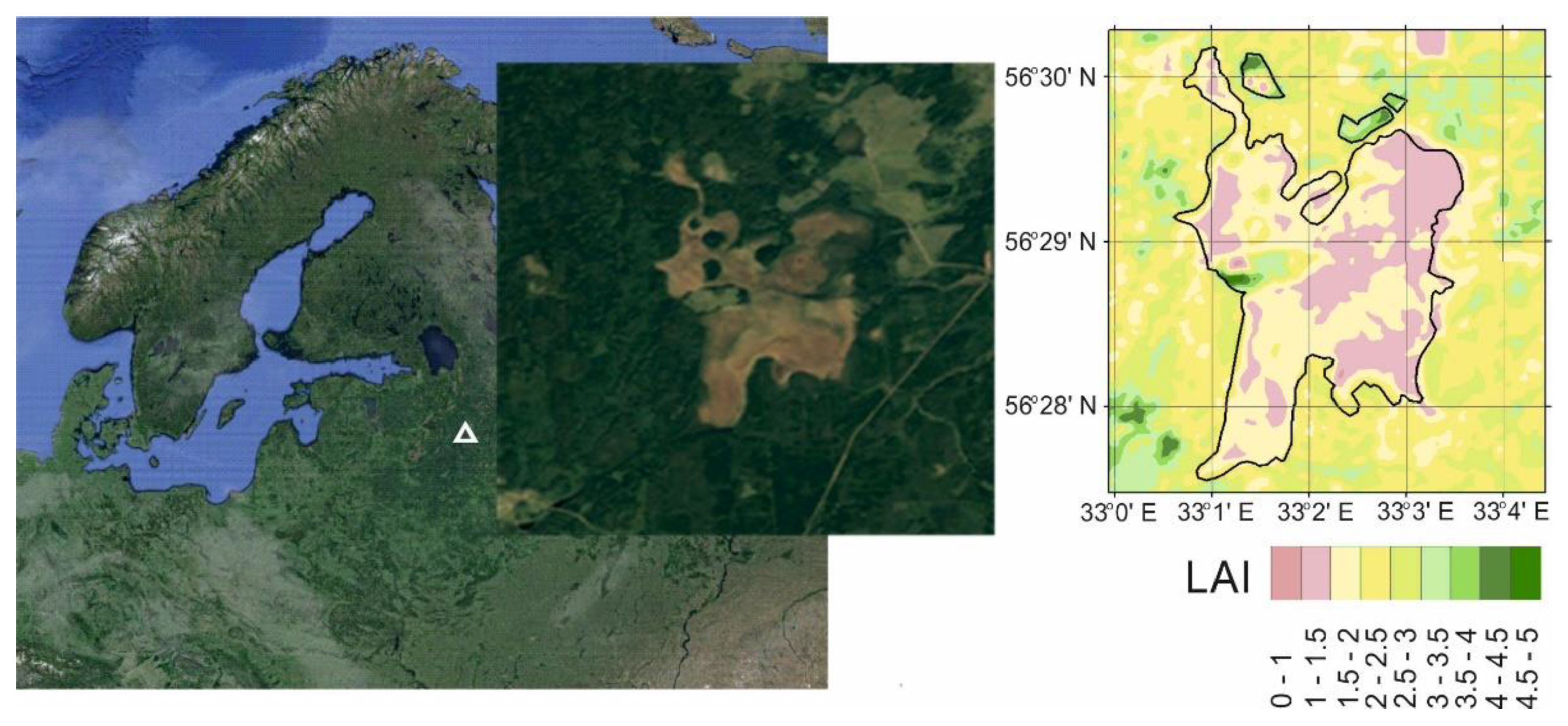
The peatland, “Staroselsky Moch”, (
Figure 1) selected for our study is situated in an area of sustainable management in the Central Forest State Natural Biosphere Reserve (CFSNBR) (56.473° N, 33.041° E). The modeling domain includes both the peatland and the surrounding forest and grassland landscapes. The total area of the modeling domain is approximately 4 km
2. The surface of the peatland is quite flat, with a small slope to the east (less than 1°). The peatland belongs to the oligotrophic type, has an irregular shape, and is characterized by mosaic vegetation.
The equipment for the meteorological and eddy covariance flux measurements was mounted at a height of 2.4 m on a 3 m tall steel tripod installed in the central part of the peatland. The eddy covariance equipment for the measurements of the vertical NEE, LE, and H fluxes included the open path CO2/H2O gas analyzer LI-7500A (LI-COR Inc., Lincoln, NE, USA) and the 3D ultrasonic anemometer CSAT3 (Campbell Scientific, Logan, UT, USA). Eddy covariance data were collected at a 10 Hz rate.
3. Results and Discussion
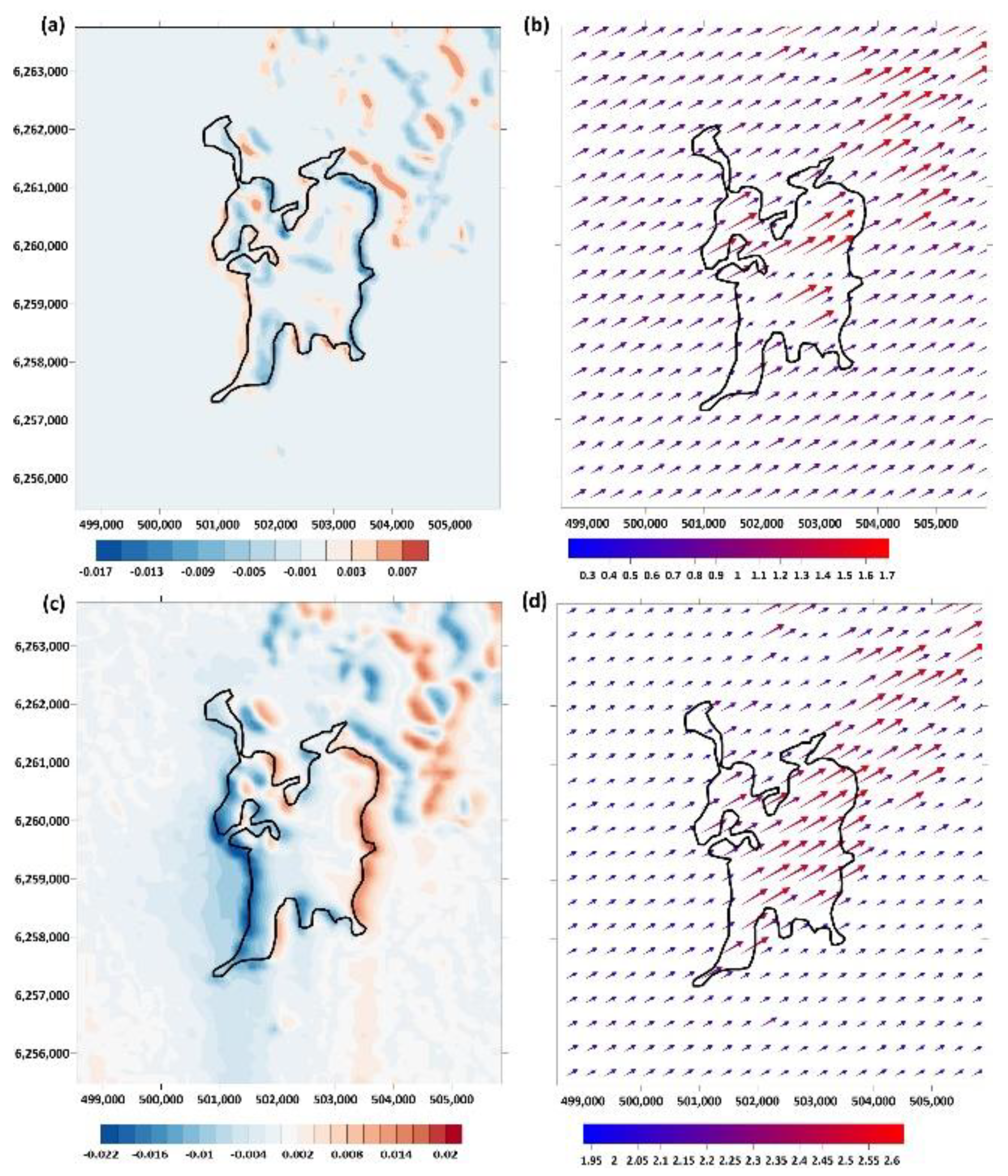
The results of the numerical experiments showed a very strong variability of wind components and CO
2 fluxes within the modeling domain.
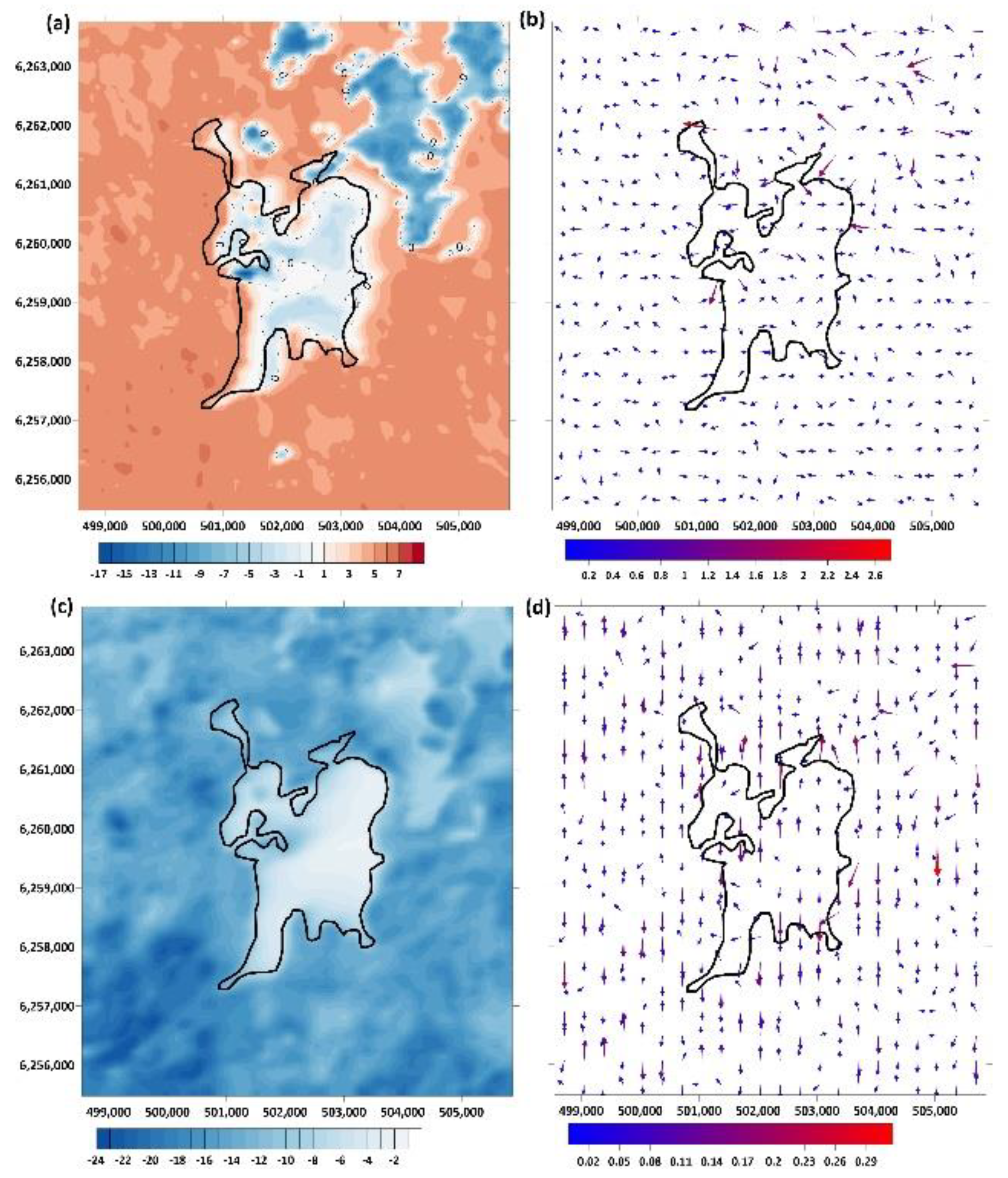
Figure 2 shows examples of the spatial distribution of the vertical and horizontal wind components at different heights above the ground surface. Examples of the model simulations of the vertical and horizontal CO
2 fluxes are shown in
Figure 3.
The mosaic and heterogeneous structure of the plant canopy results in a large heterogeneity of the spatial wind distribution. The largest anomalies of the vertical wind components were found at the boundaries of various communities and, particularly, at the wind- and lee-ward forest boundaries. At the same time, the modeling results showed insignificant changes of the wind direction at different heights above the ground surface. It was shown that the downward air flows at the windward and upward air-flows at the leeward forest boundaries arise near the ground surface. The vertical air-flows above the tree crowns have opposite directions.
Comparisons of modeled and measured (eddy covariance) vertical CO2 fluxes in the central part of the peatland at the flux tower location and at a height of 3 m above the surface showed very good agreement between the modeled and measured fluxes. At the same time, the modeled vertical CO2 fluxes at a height of 30 m above the ground surface are somewhat larger compared with the eddy flux measurement at a 3 m level. This obviously resulted from the horizontal CO2 advection from the surrounding forests. In particular, the modeling results showed that, whereas the vertical fluxes above a forest canopy at a 30 m height ranged between −12 and −24 µmol m−2 s−1, the vertical CO2 fluxes above the peatland are some smaller and varied in the central part (between −2 µmol m−2 s−1 and −12 µmol m−2 s−1), that is, they are somewhat higher than at the lower modeling layers (e.g., 3 m).
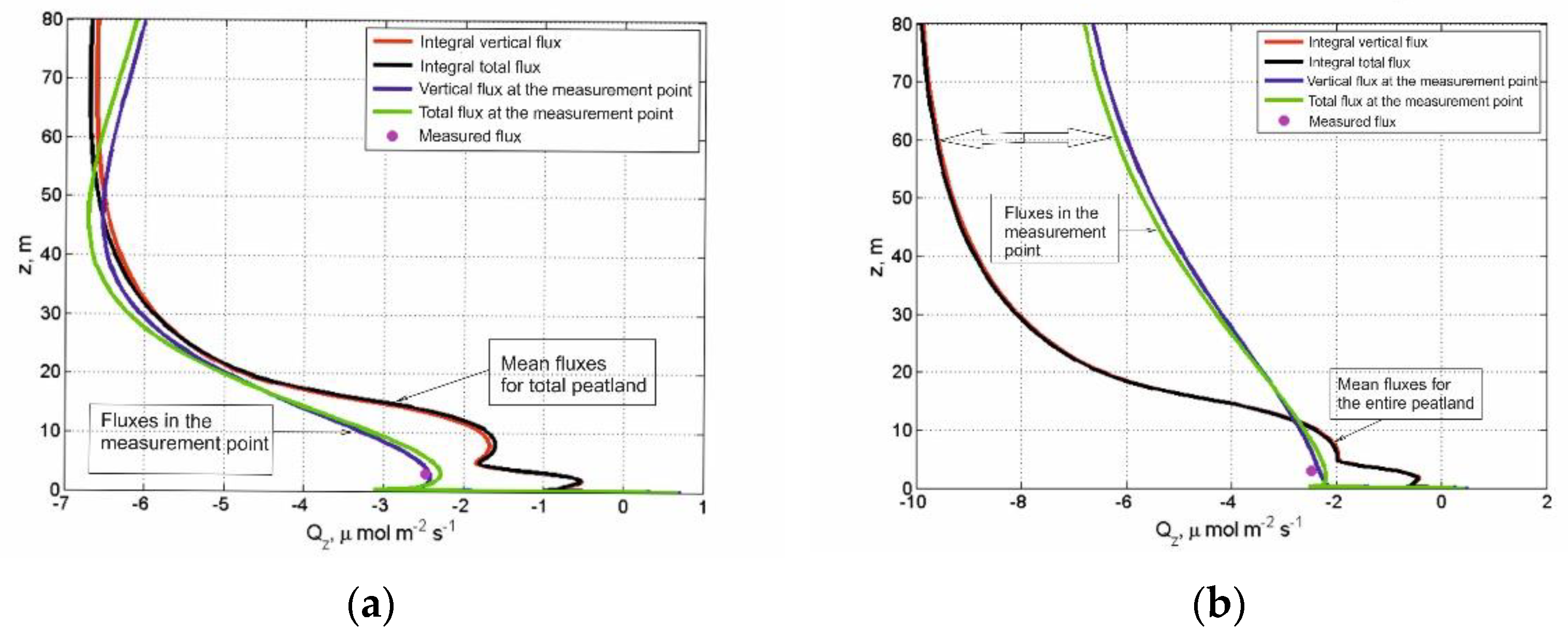
The large spatial flux heterogeneity makes it very difficult to apply the up-scaling of the point flux measurements (e.g., the eddy covariance) to the entire peatland area. The modeling results show a large difference between the calculated vertical CO
2 flux profiles at the flux tower site and the averaged vertical CO
2 flux profiles calculated by integrating the local profiles over the entire peatland area (
Figure 4). The difference between the flux tower and the entire peatland profiles changed depending on the height above the ground surface and the prevailing wind direction.
4. Conclusions
A hydrodynamic model was developed and applied to describe the spatial patterns of wind velocity and vertical and horizontal CO2 fluxes above a spatially inhomogeneous peatland, the “Staroselsky Moch”. The results showed a significant heterogeneity of the air flow distributions within both the peatland and the surrounding forest. The sharpest changes of vertical and horizontal wind components were found at the windward and leeward forest edges. At the forest edges, the maximum rates of the horizontal CO2 fluxes were also detected.
Comparisons of the modeled fluxes for the central part of the peatland with the eddy covariance flux measurements showed good agreement. A large spatial vegetation heterogeneity within the peatland and the non-uniform surrounding forest make it impossible to perform a simple extrapolation of the eddy covariance data to apply to the entire peatland area. The 3D model, in this case, can be a very effective tool for regional flux up-scaling.
Author Contributions
Conceptualization, A.O. and I.M.; methodology, A.O., I.M. and J.K.; software, I.M.; validation, I.M.; investigation, I.M., A.O. and J.K.; data curation, J.K. and A.O.; writing—original draft preparation, I.M.; writing—review and editing, A.O.; visualization, I.M. supervision, A.O.; project administration, A.O.; funding acquisition, A.O. All authors have read and agreed to the published version of the manuscript.
Funding
This research was funded by Lomonosov Moscow State University (grant number AAAA-A16-116032810086-4).
Institutional Review Board Statement
Not applicable.
Informed Consent Statement
Not applicable.
Data Availability Statement
The data presented in this study are available on request from the corresponding author.
Conflicts of Interest
The authors declare no conflict of interest.
References
- Aubinet, M.; Vesala, T.; Papale, D. Eddy Covariance: A Practical Guide to Measurement and Data Analysis; Springer: Dordrecht, The Netherlands, 2012; p. 438. [Google Scholar]
- Sellers, P.; Dickinson, R.E.; Randall, D.A.; Betts, A.K.; Hall, F.G.; Berry, J.A.; Collatz, G.J.; Denning, A.S.; Mooney, H.A.; Nobre, C.A.; et al. Modeling the exchanges of energy, water, and carbon between continents and the atmosphere. Science 1997, 275, 502–509. [Google Scholar] [CrossRef] [PubMed]
- Vager, B.; Nadezhina, E. Atmospheric Boundary Layer in Conditions of Horizontal Non-Uniformity; Gidrometeoizdat: Leningrad, Russia, 1979. (In Russian) [Google Scholar]
- Penenko, V.; Aloyan, A. Models and Methods for Environmental Protection Problems; Nauka: Moscow, Russia, 1985. (In Russian) [Google Scholar]
- Sogachev, A.; Panferov, O. Modification of two-equation models to account for plant drug. Bound. Lay. Meteorol. 2006, 121, 229–266. [Google Scholar] [CrossRef]
- Sullivan, P.P.; McWilliams, J.C.; Moeng, C.-H. A subgrid-scale model for large-eddy simulation of planetary boundary-layer flows. Bound.-Layer Meteorol. 1994, 71, 247–276. [Google Scholar] [CrossRef]
- Wyngaard, J.C. Turbulence in the Atmosphere; Cambridge University Press: Cambridge, UK, 2010. [Google Scholar]
- Dubov, A.S.; Bykova, L.P.; Marunich, S.V. Turbulence in Vegetation Canopy; Gidrometeoizdat: Leningrad, Russia, 1978. (In Russian) [Google Scholar]
- Mukhartova, Y.V.; Dyachenko, M.S.; Mangura, P.A.; Mamkin, V.V.; Kurbatova, J.A.; Olchev, A.V. Application of a three-dimensional model to assess the effect of clear-cutting on carbon dioxide exchange at the soil-vegetation-atmosphere interface. IOP Conf. Ser. Earth Environ. Sci. 2019, 368, 012036. [Google Scholar] [CrossRef]
- Mukhartova, Y.V.; Mangura, P.A.; Levashova, N.T.; Olchev, A.V. Selection of boundary conditions for modeling the turbulent exchange process within the atmospheric surface layer. Comput. Res. Model. 2018, 10, 27–46. (In Russian) [Google Scholar] [CrossRef]
- Ball, J.T.; Woodrow, I.E.; Berry, J.A. A model predicting stomatal conductance and its contribution to the control of photosynthesis under different environmental conditions. In Progress in Photosynthesis Research; Springer: Dordrecht, The Netherlands, 1987; pp. 221–224. [Google Scholar]
- Leuning, R. A critical appraisal of a combined stomatal-photosynthesis model for C3 plants. Plant Cell Environ. 1995, 18, 339–355. [Google Scholar] [CrossRef]
- Oltchev, A.; Ibrom, A.; Constantin, J.; Falk, M.; Richter, I.; Morgenstern, K.; Joo, Y.; Kreilein, H.; Gravenhorst, G. Stomatal and surface conductance of a spruce forest: Model simulation and field measurements. J. Phys. Chem. Earth. 1998, 23, 453–458. [Google Scholar] [CrossRef]
| Publisher’s Note: MDPI stays neutral with regard to jurisdictional claims in published maps and institutional affiliations. |
© 2022 by the authors. Licensee MDPI, Basel, Switzerland. This article is an open access article distributed under the terms and conditions of the Creative Commons Attribution (CC BY) license (https://creativecommons.org/licenses/by/4.0/).


