COSMO-CLM Russian Arctic Hindcast, 1980–2016: Surface Wind Speed Evaluation and Future Perspectives ^†

Abstract

The surface wind speed reproduction by the novel COSMO-CLM Russian Arctic hindcast, with a ~12 km grid size, for the period 1980–2016, was evaluated in this study, according to station and satellite data. The mean wind speed was well reproduced by the hindcast, while the errors related mainly to cases when the wind speed was overestimated by the model data, up to 2 m/s. However, the extreme values (0.95 and 0.999 quantiles), according to the hindcast, were underestimated to up to −5–−10 m/s. The evaluation, according to the SAR Radarsat-2, high-resolution satellite images, including the FSS score, revealed the hindcast’s capability to reproduce β-mesoscale processes, unlike the γ-scale processes. For all 5 m/s threshold-exceeding features, a ~45 km resolution was enough for the relevant reproduction by the hindcast. At the same time, the given model grid size (~12 km) was not sufficient to reproduce extreme wind speeds, exceeding 20 m/s. Future perspectives of the COSMO-CLM Russian Arctic hindcast include the evaluations of diurnal cycles; wind speed trends; satellite data analysis for other regions of the Russian Arctic; the focus on extreme and severe events’ statistics evaluation; and quality estimation, based on other high-resolution, recent datasets.

1. Introduction

The Arctic is one of the regions of the world that is most vulnerable to climate change. On average, warming in the Arctic occurs two to four times faster than in the entire globe [1]. It is assumed that the cause of this phenomenon lies in a whole complex of physical processes, most of which are closely related to a sharp decrease in sea ice cover [2,3]. However, the regional features of Arctic warming are significantly different and need to be clarified and detailed [4]. Freeing the surface of the Arctic Ocean from sea ice contributes to an increase in extreme winds frequency [5]. Considering the corresponding growing number of severe weather events in the Arctic and the prospects for the development of the Arctic coast and the Northern Sea Route, it is necessary to study, in detail, the observed climate changes in the Russian Arctic, involving climatic information with fine spatial resolution.

Most of the existing hydrometeorological datasets for the Arctic region are either fragmentary (station and expeditionary observations) or have coarse spatial resolution (tens of kilometres—climate datasets, reanalyses, etc.) or limited temporal coverage (satellite data), which does not allow them to resolve many dangerous phenomena or to study their statistical characteristics based on long-term timeseries. The novel, detailed COSMO-CLM Russian Arctic hindcast, covering the period between 1980–2016, with a ~12 km grid size [6], allowed us to investigate the features of regional Arctic climate changes in more detail, including the surface wind speeds and spatial patterns. However, it is very important to evaluate this dataset according to independent observational data sources, including stations and satellites. Therefore, the main tasks were to reveal its regional advantages, shortcomings and sources of errors, and to obtain estimates of spatial scale that were sufficient to resolve different severe events.

2. Materials and Methods

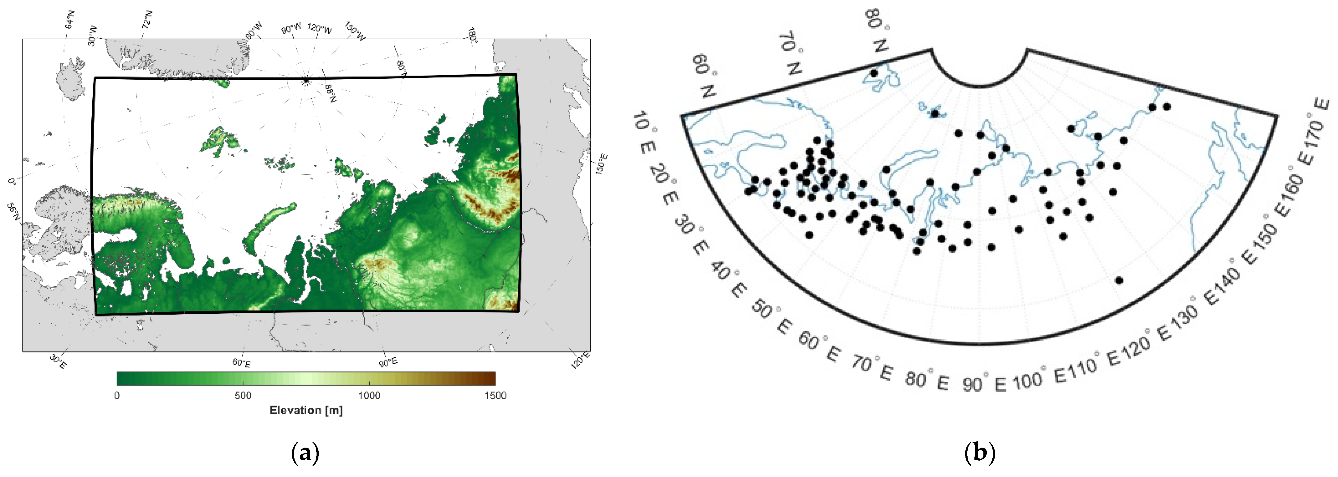
2.1. COSMO-CLM Russian Arctic Hindcast

The COSMO-CLM Russian Arctic hindcast, which included approximately a hundred different hydrometeorological characteristics at both surface and model levels (50 levels), was created by the long-term regional atmospheric hydrodynamic simulation, based on the COSMO-CLM ver. 5.05 model. It covered the Barents Sea, Kara Sea, and the Laptev Sea, with grid size 0.108° (~12 km) (Figure 1a). The ERA-Interim reanalysis was used as initial and boundary conditions in the final experiments’ configuration [7], including the spectral nudging technique. Primary assessments of the obtained meteorological data archive showed the adequacy of its reproduction of the main climatological patterns of the average surface wind speeds. Furthermore, the details of the distribution of wind speed are manifested in many regions of the Arctic, according to the COSMO-CLM Russian Arctic hindcast, which is not reflected in the parental ERA-Interim global dataset [6].

Simulations were performed using the shared research facilities of the high-performance computing resources at Lomonosov Moscow State University: supercomputer “Lomonosov-2” [8]. The output step for all variables was 1 h and the total volume of data was approximately 120 TB. The COSMO-CLM Russian Arctic hindcast data are partially available on the FigShare repository for periods, 1980–2008 and 2010–2016 [9] and include information on the most important surface fields: 2 m air temperature and humidity, sea level pressure, 10 m wind speed components, surface radiation and turbulence fluxes, and precipitation with 3-hourly timestep. Surface 10 m wind speed component timeseries were used in this study. For more detailed information on the hindcast creation and its first evaluations, please see [6,7].

2.2. Weather Stations’ Data

Weather stations’ data were used to assess the quality of the reproduction of 10 m wind speeds. There are data timeseries for 95 stations from the Russian Research Institute for Hydrometeorological Information—World Data Centre [10], for the period 1980–2016. All these stations are provided in Figure 1b. The nearest model grid was selected for each weather station according to their coordinates, taking into account the model land–sea mask. The selected grids were used for further comparisons.

2.3. Satellite Data

Synthetic aperture radar (SAR) images from Radarsat-2 satellite were used in this study for the area of Novaya Zemlya, since this region is well known for developing downslope windstorms [11] and for having among the most extreme wind speeds in the Arctic region. The SAR data were downloaded from the NOAA public archive [12]. Nineteen images with a spatial resolution of 2.5 km were selected from the available images for the period from 2014 to 2016, with the most recognizable structure of the wind speed field and after applying the masks for land and ice. Separately, the 2–23 m/s wind speed limits were set manually to eliminate possible errors associated with sea ice surface interpretation. The edges of the image were also cropped since there were data distortions observed along them. Hindcast data were selected for comparison with satellite data satisfying the time difference condition no more than 30 min. Next, both model and satellite data were interpolated onto a common, regular 5 km grid using the quadratic inverse distance method. Model grid points lacking corresponding satellite data, due to the use of different masks, were also excluded from the hindcast wind speed data to perform a correct comparison.

2.4. Methods

To compare the selected data sources with the hindcast, the following statistics were calculated: the differences between the hindcast and station values (or satellite data), the biases, and RMSE and correlation coefficients for these differences, representing model errors. The quantiles 0.95, 0.99, and 0.999 were calculated for the stations (or satellite data) and for the corresponding model grid points, as well as the differences between them, to study the extreme values of wind speed.

The Fraction Skill Score (FSS) method [13] was applied for spatial comparisons between SAR images and hindcast data. The spatial verification methods allowed us to estimate the wind speed pattern reproduction in more complete and convenient ways, and to assess spatial resolution required to capture mesoscale features, according to different wind speed intervals.

Firstly, model and satellite data were interpolated on the common ~5 km grid. Further, the wind speed thresholds were defined as 5, 10, 15, and 20 m/s. For each threshold and data source, binary fields were created according to the following: «1» was the value above the given threshold, and «0» was below it. Next, the number of grids having value of 1 in the neighbourhood of each point in the binary fields were computed separately for model and satellite data. The neighbourhood sizes n = 1, 3, 5, 7, and 9 grid cells were used in this study. In this way, fractions for each square length and each wind speed threshold were calculated, and then the FSS value was calculated, following formulas (1)–(5), as follows:

$$O\left(n\right)\left(i,j\right)=\frac{1}{n^2}{\displaystyle \sum }_{k=1}^n{\displaystyle \sum }_{l=1}^n{I}_O\left[i+k-1-\frac{\left(n-1\right)}{2},j+l-1-\frac{\left(n-1\right)}{2}\right]$$

(1)

$$M\left(n\right)\left(i,j\right)=\frac{1}{n^2}{\displaystyle \sum }_{k=1}^n{\displaystyle \sum }_{l=1}^n{I}_M\left[i+k-1-\frac{\left(n-1\right)}{2},j+l-1-\frac{\left(n-1\right)}{2}\right]$$

(2)

$$MSE\left(n\right)=\frac{1}{N_X{N}_Y}{\displaystyle \sum }_{i=1}^{N_X}{\displaystyle \sum }_{j=1}^{N_Y}{\left[O_{\left(n\right)i,j}-M_{\left(n\right)i,j}\right]}^2$$

(3)

$$FS{S}_{\left(n\right)}=1-\frac{MS{E}_{\left(n\right)}}{MS{E}_{\left(n\right)ref}}$$

(4)

$$MS{E}_{\left(n\right)ref}=\frac{1}{N_X{N}_Y}\left[{\displaystyle \sum }_{i=1}^{N_X}{\displaystyle \sum }_{j=1}^{N_Y}{O}^2{}_{\left(n\right)i,j}+{\displaystyle \sum }_{i=1}^{N_X}{\displaystyle \sum }_{j=1}^{N_Y}{M}^2{}_{\left(n\right)i,j}\right]$$

(5)

Here, n—neighbourhood size; I_O and I_M—binary fields from satellite observations and model data, accordingly; i goes from 1 to N_X and j goes from 1 to N_Y—total number of columns and rows—accordingly.

The FSS value varied from 0 (worst) to 1 (best), FSS > 0.5 indicated a good reproduction [14] and was applied to estimating the optimal spatial size to reproduce wind speeds within different thresholds. The larger the spatial size of n, the smoother the reproduced pattern was, and no detailed structure was captured. However, if n is too small, it would be more sensitive to the feature’s contours and its displacements, therefore, its edges would be more fragmented and could not be captured by the model. Therefore, the goal of this FSS method was to estimate an optimal spatial size for each wind speed threshold.

3. Results

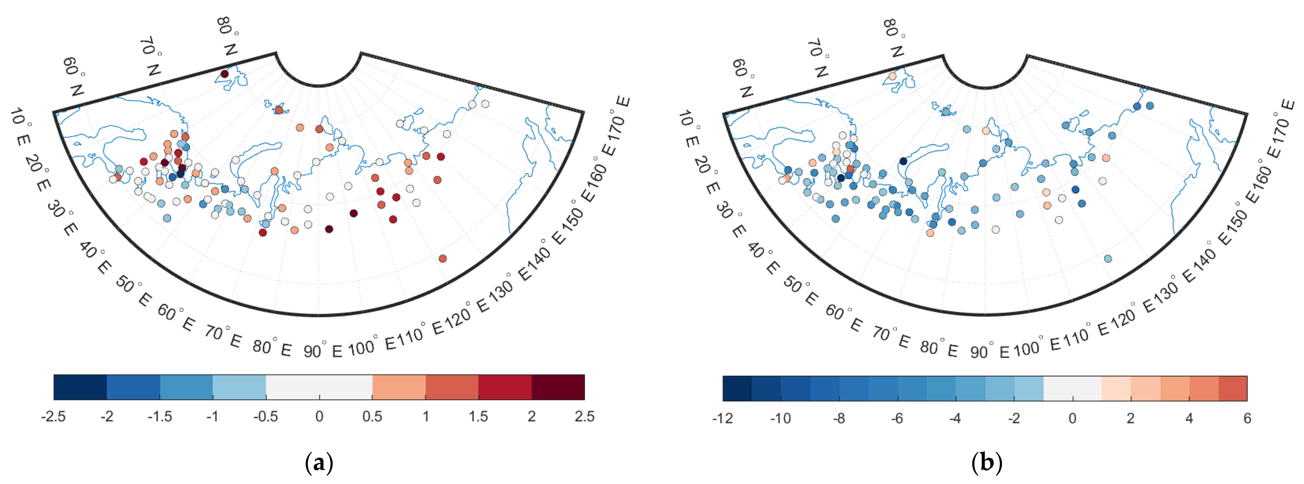
3.1. Wind Speed Errors

The comparison with the station data showed that the mean wind speed was well reproduced by the COSMO-CLM hindcast, while the errors related mainly to cases when the wind speed was overestimated by the model data, up to 2 m/s. There were also a sufficient number of stations where the difference between the hindcast and the station data was close to zero (Figure 2a). In particular, it is important to note that at three stations with the highest known average wind speeds—Malye Karmakuly, Tiksi, and Dikson Island—the average error values really tend to zero. Unlike the average wind speed, the extreme values, according to the hindcast, were underestimated, compared to the stations’ data, with up to −5 m/s for 0.95 quantiles and up to −10 m/s for 0.999 quantiles (Figure 2b).

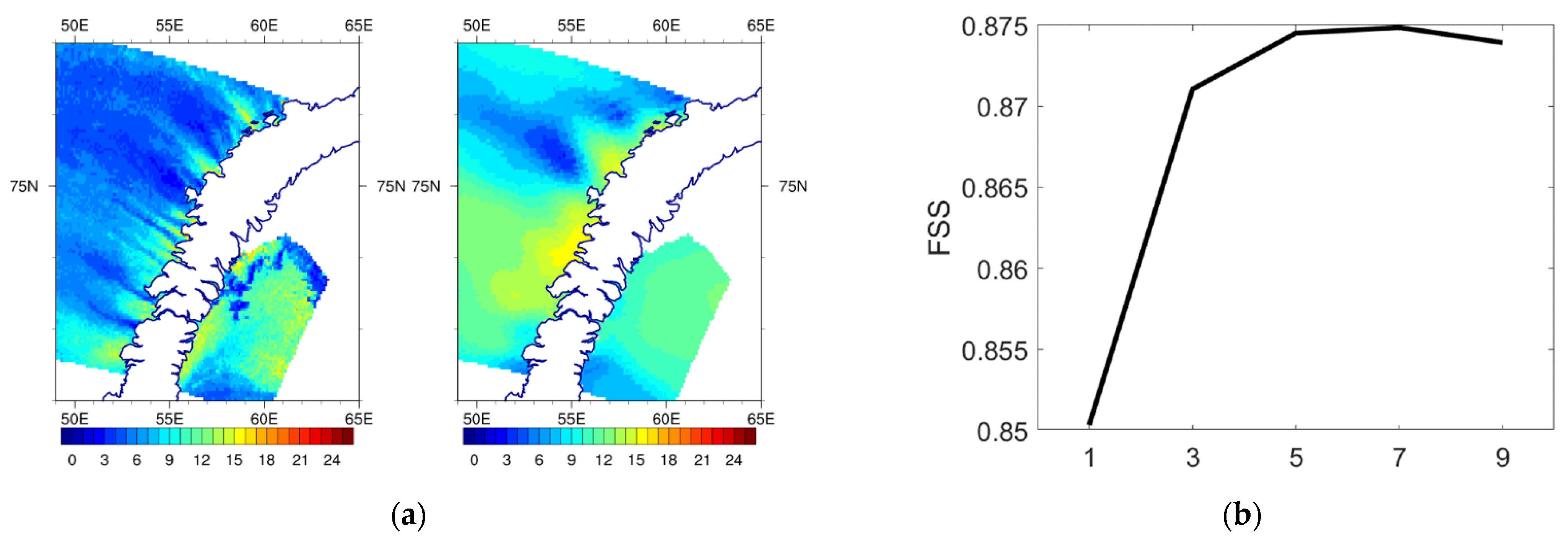
3.2. SAR Images’ Verification, Including FSS

The SAR images’ comparison with the hindcast wind speed data showed that the moderate wind speed values were often overestimated by the model; however, the differences between the quantiles showed that the more extreme the observed wind speed was, the greater the probability of underestimation by the model was. The model reproduced the contour and intensity of the feature well, however, its size could be larger than it really was, due to the model’s grid size restrictions. The evaluation of the SAR images, according to the FSS score for specific extreme wind speed cases near the Novaya Zemlya Island, showed that the hindcast could capture the spatial structure of wind speeds higher than 10 m/s and, partially, than 15 m/s, however, it could not reproduce 20 m/s features. The FSS analysis revealed that the COSMO-CLM Russian Arctic hindcast was successful in 5 m/s feature reproduction, because ~45 km size was sufficient (Figure 3). However, the given model resolution (~12 km) was not sufficient to reproduce extreme wind speeds, exceeding 15 and 20 m/s, although the 20 m/s threshold was reproduced by the model for one case out of 19 (on 7 December 2014).

4. Discussion

4.1. Sources of Errors for Wind Speed, According to Stations

An additional study for some stations showed that the source of the abovementioned errors in the surface wind speed could be caused by differences in the height and distance between the stations and the corresponding model grid points. The examples of the wind speed errors include the stations at Zimnegorsky Mayak and Sosnovets Island, with the largest underestimation by the model. The stations are located on the coast or small island, and are not resolved by the model orography interpreting the surface as a continent. Most of the stations where the model overestimated the wind speeds significantly, were situated in Siberia. There was another source of errors linked to the model’s surface orography smoothing over mountain ranges and valleys, which could have led to the reproduction of higher wind speeds. The specific task that will be solved in future studies, is to implement any vertical corrections of wind speeds to reduce these errors, specifically over eastern Siberia’s mountainous region.

4.2. Discussion of FSS Method Results

Generally, the 5 m/s threshold was reproduced by the hindcast perfectly, with maximal FSS > 0.5. However, the higher threshold, the lower FSS, and smaller number of cases: e.g., for the 10 m/s threshold there were seven cases with FSS > 0.45; 13 cases were with FSS = 0 for 15 m/s; and only one case was with non-zero FSS for 20 m/s with maximal FSS = 0.12. The latter case indicates that such features were not captured by the model with given spatial sizes, it is beyond the model capability. It is worth mentioning that the number of grids required for successful model reproduction reduced with an increase in the wind speed threshold corresponding to the decrease in the spatial scale, when higher wind speeds were observed. This suggests the quantitative assessment of spatial scales could be resolved by the COSMO-CLM Russian Arctic hindcast. This result confirmed the model’s capability to reproduce β-mesoscale processes, unlike the γ-scale processes, which are associated with larger wind speed threshold values.

5. Conclusions

The evaluation of the COSMO-CLM Russian Arctic hindcast showed that the average wind speed was well reproduced, with a slight overestimation of the mean wind speed. The quantile differences indicated that extreme wind speeds were underestimated: the error ranged from −2 to −10 m/s for 0.95 and 0.999 quantiles, respectively.

The FSS analysis applied to the SAR satellite images revealed that the hindcast was successful in the reproduction of features exceeding the 5 m/s threshold, with a ~45 km resolution. However, the given model grid size (~12 km) was not sufficient to reproduce extreme wind speeds, exceeding 15 and 20 m/s. The number of grids necessary for a successful model reproduction reduced with an increase in the wind speed threshold, which corresponded to a decrease in spatial scale when higher wind speeds were observed.

Future perspectives of the COSMO-CLM Russian Arctic hindcast should include the evaluation of diurnal cycles; wind speed trends; satellite data for other regions of the Russian Arctic; hindcast prolongation to 2019; sharing more data online. The focus could be also on the statistical evaluation of extreme and severe events (downslope windstorms and polar lows’ climatology, using satellite data); and quality estimation, based on other datasets (e.g., ERA5, CARRA, satellites’ climatology, etc.).

References

1. Masson-Delmotte, V.; Zhai, P.; Pirani, A.; Connors, S.L.; Péan, C.; Berger, S.; Caud, N.; Chen, Y.; Goldfarb, L.; Gomis, M.I.; et al. (Eds.) IPCC, 2021: Climate Change 2021: The Physical Science Basis. Contribution of Working Group I to the Sixth Assessment Report of the Intergovernmental Panel on Climate Change; Cambridge University Press: Cambridge, UK; New York, NY, USA, 2021; in press. [Google Scholar] [CrossRef]
2. Brennan, M.K.; Hakim, G.J.; Blanchard-Wrigglesworth, E. Arctic Sea-Ice Variability During the Instrumental Era. GRL 2020, 47, 7. [Google Scholar] [CrossRef]
3. Walsh, J.E.; Fetterer, F.; Scott Stewart, J.; Chapman, W.L. A database for depicting Arctic sea ice variations back to 1850. Geogr. Rev. 2017, 107, 89–107. [Google Scholar] [CrossRef]
4. Maksym, T. Arctic and Antarctic Sea Ice Change: Contrasts, Commonalities, and Causes. Annu. Rev. Mar. Sci. 2019, 11, 187–213. [Google Scholar] [CrossRef]
5. Moore, G.W.K.; Renfrew, I.A. Tip jets and barrier winds: A QuikSCAT climatology of high wind speed events around Greenland. J. Clim. 2005, 18, 3713–3725. [Google Scholar] [CrossRef]
6. Platonov, V.; Varentsov, M. Introducing a New Detailed Long-Term COSMO-CLM Hindcast for the Russian Arctic and the First Results of Its Evaluation. Atmosphere 2021, 12, 350. [Google Scholar] [CrossRef]
7. Platonov, V.; Varentsov, M. A new detailed long-term hydrometeorological dataset: First results of extreme characteristics estimations for the Russian Arctic seas. IOP Conf. Ser. Earth Environ. Sci. 2020, 611, 012044. [Google Scholar] [CrossRef]
8. Voevodin, V.; Antonov, A.; Nikitenko, D.; Shvets, P.; Sobolev, S.; Sidorov, I.; Stefanov, K.; Voevodin, V.; Zhumatiy, S. Supercomputer Lomonosov-2: Large Scale, Deep Monitoring and Fine Analytics for the User Community. Supercomp. Front. Innov. 2019, 6, 4–11. [Google Scholar] [CrossRef]
9. Data from the COSMO-CLM Russian Arctic Hindcast, Figshare. Available online: https://figshare.com/collections/Arctic_COSMO-CLM_reanalysis_all_years/5186714 (accessed on 13 June 2022).
10. Russian Research Institute for Hydrometeorological Information—World Data Center. Available online: http://aisori-m.meteo.ru/ (accessed on 13 June 2022).
11. Shestakova, A.A.; Toropov, P.A.; Matveeva, T.A. Climatology of extreme downslope windstorms in the Russian Arctic. WACE 2020, 28, 100256. [Google Scholar] [CrossRef]
12. SAR Radarsat-2 Data. Available online: https://www.ncei.noaa.gov/data/oceans/sar-winds/ (accessed on 13 June 2022).
13. Roberts, N.M.; Lean, H.W. Scale-selective verification of rainfall accumulations from high-resolution forecasts of convective events. Mon. Weather Rev. 2008, 136, 78–97. [Google Scholar] [CrossRef]
14. Skok, G.; Roberts, N. Analysis of fractions skill score properties for random precipitation fields and ECMWF forecasts. Quar. J. R. Met. Soc. 2016, 142, 2599–2610. [Google Scholar] [CrossRef]
Figure 1. COSMO-CLM Russian Arctic hindcast area [6] (a) and weather station locations selected in this study (b).
Environsciproc 19 00039 g001
Figure 2. Mean errors for hindcast wind speed according to station data (a), m/s; difference between hindcast and station data in 0.999 quantiles (b), m/s.
Environsciproc 19 00039 g002
Figure 3. SAR (left) and hindcast (right) wind speed data, interpolated on the common grid after applying land and sea ice masks, m/s (a); FSS score plot with regard to number of grid points (size n) for 5 m/s threshold, (b) for 28 November 2015 case.
Environsciproc 19 00039 g003
Publisher’s Note: MDPI stays neutral with regard to jurisdictional claims in published maps and institutional affiliations.