A Comparative Study for Provision of Environmental Flows in the Tapi River

Abstract

Environmental flows are defined as the flow required into a stream to maintain the river’s ecosystem. The notion of Environmental Flow Allocation (EFA) ensures that a sufficient amount of water is delivered to the stream to maintain ecological integrity. The objective of this study is to examine environmental flows and determine the best acceptable strategy for providing flows into the river in the Lower Tapi Basin. To achieve this objective, daily discharge data from three sites, Ukai (period 1975–2020), Motinaroli (period 1990–2021), and Ghala (period 1995–2005) were collected and analyzed using the Tennant, Tessman, variable monthly flow (VMF), and Smakhtin methodologies. A comparative analysis was carried out on all three sites using the four methodologies. The Tessman and VMF approaches have a strong connection with the computed environmental flow requirements (EFR), according to the results. The calculated EFR was found to be in the range of 30–35% of mean annual flows (MAF). The maximum EFR found at station Ghala is about 54.5% of MAF according to the Tessman method. Such research will help to prevent future degradation of the river by supplying flow in accordance with the EFR, and it will also be used by stakeholders and policymakers to allocate water to preserve the ecosystem.

1. Introduction

Rivers constitute one of the major parts of the water cycle on the earth and carry basic natural requirements of all the natural life events and ecosystem functions. Since the beginning of time, people have been fascinated by rivers because they rely on them for their water supply, and, as a consequence, the earliest human civilizations developed along the rivers and gradually started to control them, draining and diverting more water as population and water demand increased [1]. In many situations, this led to some rivers having almost no amount of flow in the dry season, causing various forms of damage to the numerous ecosystem services that river water provides. The loss of feeding and breeding habitats in the floodplain water bodies due to the construction of embankments and increased silt load and macrophyte growth are major causes for declining fish resources. In fact, wetlands, rivers, and lakes support a very large share of biodiversity on Earth, even though freshwater ecosystems account for a negligible (0.01%) amount of the planet’s water and a small portion of its surface [2].

In this context, the concept of environmental flows emerges as discussions increasingly expanded to cover a wide range of subjects, such as the geomorphic, sediment movement, aquatic habitat, and the needs of species other than fish. Environmental flows are defined in a variety of ways. The widely cited Brisbane Declaration states [3], “Environmental flows (EFs) are the quantity, timing, duration, frequency, and quality of flows required to sustain freshwater, estuarine, and near shore ecosystems and the human livelihoods and wellbeing that depend on them”. Environmental flows are most often associated with the concept of uninterrupted flow or river connectivity longitudinally and laterally between the stream and riverbanks. The river is a pathway for the movement of nutrient content, soil particles, and aquatic species from upstream to downstream, as well as a medium for the transportation of water and energy. Moreover, in a river, aquatic flora and fauna can move in upstream directions as well as downstream directions. If the river does not have a sustainable amount of flow for an extended period, all these flows will stop. On the contrary, floodwaters disperse out from the mainstream and saturate the adjacent plain of flood at specific times and frequencies. This helps in the formation of a hydraulic link between the banks of the water and the river’s waterway, allowing food, nutrients, and carbon to cross-subsidize the ecosystem [4]. A river’s hydraulic link to its floodplains is one of the essential driving forces for major biota interactions, productivity, and diversity in the river and its floodplain. This illustrates that EFs can be seen as the lateral requirements of the concept of flood pulse [5] and methodology for delivering the longitudinal requirements notion of river continuity [6]. Several countries have recently incorporated the EFs into the water management concept. For example, South Africa’s water law recognizes the importance of water for environmental maintenance prioritized alongside water for basic human needs [7], and Tanzania has also adopted this concept [8]. The USA’s Clean Water Act of 1972 establishes the goal of restoring and preserving the chemical, physical, and ecological integrity of a nation’s water, while the UK’s Water Resources Act of 1963 mandated a minimum number of acceptable flows to maintain natural beauty and fisheries [9]. Environmental flows are, additionally, a main research focus for important international organizations such as the World Bank [10] and the International Union for the Preservation of Nature (IUCN) [11].

Environmental Flows Assessments provide a time series of data on the relationships between the flows of the river and river wellbeing. They describe the expected basin-wide ecological and social outcomes connected to scenarios of various water management options in their most extensive type. EFs are a particular set of discharges of a specific magnitude, specific frequency, and specific timing that are required to verify a significant range of river benefits to protect the environment. Varying frequency of high flows is necessary for stream protection, bird spawning, algae regulation, floodplain coastal floods, and preservation of riparian vegetation. Medium flows may be crucial for the cycling process of organic compounds from banks of the river and for aquatic habitats, whereas low discharge of flows of varying values are required for fish reproduction, preservation of quality of water. Nowadays, many authors claim that social factors and cultural factors, such as human well-being, should be included in EF [12].

EFs can be calculated for several purposes. The most common is to prevent further deterioration of a river or to rehabilitate a degraded river to a better ecological state [13]. EFs are typically estimated near key man-made features (previous, existing, or predicted) in river flow characteristics caused by water long-term storage or diversion. In particular, EF is usually estimated at specific locations and conditions, like downstream of dam or at upstream of any big city, etc. As an example, significant changes in water quality can be caused by changes in the upstream watershed, such as large-scale withdrawals from surface or groundwater sources [14]. Moreover, over many centuries, storage reservoirs have been used to regulate river flows by diverting and releasing water to fulfill the needs of the service area. As a result, estimating EF requirements just downstream of the dam or a point of diversion is very common. Other possible locations include areas just downstream of a major city or industry or at the entrance of a wildlife refuge if a river runs through it. Water flowing to the sea was seen as “wasted” in India, as it was in much of the rest of the globe. River waters were channeled through dams and other structures to the greatest extent physically possible [15]. Even the current National Water Policy places “ecology” fourth on the list of water-allocation objectives. In the Indian context, primarily hydrologic methods are used to define environmental flows in rivers. As the progressive destruction of the water environment became apparent, environmental concerns began to gain traction. The issues of EF assessment and management are high on the world agenda at present time. At this time, it remains a new research field. In many countries, including India, there has not even been a nationwide assessment of the water requirements of rivers and their associated aquatic ecosystems. Countries like India, which are also dealing with high population growth nowadays, also have to deal with the allocation of water for irrigation and drinking water purposes making it difficult to allot water to maintain the environmental flow as it is actually needed.

In this context, this study aims to find the environmental flow requirements (EFRs) for the Tapi River (India) by using four different methods, trying to find the best-fitted method among all. The result of the study helped the Ukai Irrigation Circle in releasing the flow from the Ukai dam site. There are significant physical changes in the river that have been observed, which is why the study area was selected. The study is helpful for the Surat Municipal Corporation for the maintenance of the river channel. The flow between the weir and mouth of the river should not have a sufficient amount of flow in the river channel. Flow in this part of the river varies to a great extent between monsoon season and non-monsoon season. This part is also affected by the river meander and sedimentation. After seeing all these problems, an assessment of the EF was required to be carried out at the site.

2. Methods Used for Assessment of Environmental Flows

Before the 1990s, water management was limited to minimum flow requirements and water quality standards. The last two decades have seen a shift in river management that is more attentive to the seasons and natural circulation regimes of interannual flow variability, as well as the magnitude, timing, and frequency of various flow conditions. According to a thorough investigation of environmental flow techniques conducted by Tharme [16], there are more than 207 significant environmental flow methodologies (EFMs) in use across 44 countries and six regions of the world. These EFMs can be broadly divided into four categories, including [17]: hydrological, hydraulic, habitat-simulation, and holistic (

Table 1. Environmental flow methodologies [18].

Category	Data	Method
Hydrological	Long-term data sets of unregulated or naturalized daily flows (>20 years)	Tennant, Tessmann, Indicators of Hydraulic Alteration (IHA), range of variability approach (RVA), Desktop Reserve Model (DRM), FDC, HAT
Hydraulic	Flow velocity, river cross-section	R2 Cross method
Habitat-simulation	Flow velocity, river cross-section, and data set of a fish specie	Physical habitat Simulation (PHABSIM), Integrated Facilities Management (IFIM)
Holistic	Combination of hydrological, hydraulics, ecological, and social sciences (expert knowledge)	building block method (BBM), Ecological Limits of Hydrological Alteration (ELOHAregimer), DRIFT model

). Figure 1 shows the graphical representation of the timeseries of the discharge data.

In particular, hydrological methods look at historical runoff series to determine natural flow conditions and advised flow rates. These methods are easy to perform and inexpensive, and they can be used for the preliminary stage of the dam construction. The method is based on the premise that there is a connection between river flow and riverbed ecosystems. The method utilizes time series data of 20–50 years (long term) for the flow of the river, with the ecological flow represented by a proportion of mean yearly flow values. hydrologic index methods include the Tessman method, Tennant method, RVA approach (range of variability), DRM (Desktops Reserve Model), FDC (flow duration curve) analysis method, and the HAT (Hydrologic Assessment Tool).

2.1. Tennant Method

This method, also known as the Montana method, is the most widely used hydrological technique in the world [19]. It was created in 1976 and has been used in a minimum of 25 countries in either its original form or by applying modification to the original form [16]. The method was specially developed to determine the needs of fish in streams of Montana. A different range of flow is given for each different stage of river condition. The flow condition is defined using a proportion of mean annual flows (MAF) for two separate six-month periods. The selection of the mean annual runoff, which only depicts run-off on an annual basis and ignores variations in flow throughout the year, is its main drawback. Many researchers have concluded that, in the monsoon period, 40% of MAF is needed and in the non-monsoon period 20% of MAF is needed to maintain good habitat conditions [16].

2.2. Tessman Method

Tennant method gives the EFR for the two different seasons. To overcome this disadvantage of the Tennant method, the Tessman method was developed [20]. The flow of a river varies greatly throughout the seasons (monsoon and non-monsoon). Therefore, the calculation of EFR by considering only MAF is not adequate and the Tessman method that considers the mean monthly flow (MMF) to determine the EFR in terms of minimum flow is more appropriate. In particular, the minimum flow is evaluated as:

$$\left\{\begin{array}{c}\mathrm{M}\mathrm{M}\mathrm{F} (if \mathrm{M}\mathrm{M}\mathrm{F}<\mathrm{M}\mathrm{A}\mathrm{F})\\ 40\mathrm{\%} \mathrm{o}\mathrm{f} \mathrm{M}\mathrm{A}\mathrm{F} (\mathrm{i}\mathrm{f} 40\mathrm{\%} \mathrm{M}\mathrm{A}\mathrm{F}<\mathrm{M}\mathrm{M}\mathrm{F}<100\mathrm{\%} \mathrm{M}\mathrm{A}\mathrm{F})\\ 40\mathrm{\%} \mathrm{o}\mathrm{f} \mathrm{M}\mathrm{M}\mathrm{F} (\mathrm{i}\mathrm{f} \mathrm{M}\mathrm{M}\mathrm{F}>\mathrm{M}\mathrm{A}\mathrm{F})\end{array}\right.$$

(1)

2.3. Variable Monthly Flow (VMF) Method

The variable monthly flow (VMF) method was proposed by Pastor [18] to explain the environmental flow requirements in global water assessments. EFRs are calculated using monthly flow, which follows the totally natural discharge variability. Flows were defined as low flows (L.F), high flows (H.F.), and intermediate flows (I.F.) on the basis of this method. The method was used to increase the protection of the freshwater ecosystem during the low-flow season with a reserve of 60% of the MMF and a minimum considered flow of 30% of the MMF during the high-flow period. This method allows stakeholders to use water during the low-flow season by losing up to 40% of the MMF. The minimum flow is evaluated as:

$$\left\{\begin{array}{c}60\% \mathrm{o}\mathrm{f} \mathrm{M}\mathrm{M}\mathrm{F} (if \mathrm{M}\mathrm{M}\mathrm{F}<40\mathrm{\%} \mathrm{M}\mathrm{A}\mathrm{F})\\ 45\mathrm{\%} \mathrm{o}\mathrm{f} \mathrm{M}\mathrm{M}\mathrm{F} (\mathrm{i}\mathrm{f} 40\mathrm{\%} \mathrm{M}\mathrm{A}\mathrm{F}<\mathrm{M}\mathrm{M}\mathrm{F}<80\mathrm{\%} \mathrm{M}\mathrm{A}\mathrm{F})\\ 30\mathrm{\%} \mathrm{o}\mathrm{f} \mathrm{M}\mathrm{M}\mathrm{F} (\mathrm{i}\mathrm{f} \mathrm{M}\mathrm{M}\mathrm{F}>80\mathrm{\%}\mathrm{M}\mathrm{A}\mathrm{F})\end{array}\right.$$

(2)

2.4. Smakhtin Method

Smakhtin considered the indices from the flow duration curve for the computation of EFR for the allocation of water into the stream. Smakhtin et al. [21] first applied this method to 128 catchment areas in different parts of the world to assess the status of exploitation of the world’s rivers with the consideration of environmental water requirements. According to this method, EFR is roughly represented by a discharge which, on average each year, is exceeded 90% of the time in order to maintain “fair” ecological conditions, and Q90 is the flow that is considered for the allocation of EFR in the stream for 90% of the year. In particular, through reviewing numerous studies on low-flow hydrology, Smakhtin et al. [21] proposed that Q90 varies between 0 and 50% of MAR.

2.5. Correlation Analysis

EFR was calculated by taking an average from all four methods and denoted as the calculated EFR. Then, the relationship between the EFR for all the methods and the calculated EFR on a monthly basis was analyzed by means of a simple linear correlation.

2.6. Summary of the Paper

In the following schematic working flow diagram, a summary of the paper with the different steps performed to detect the EFR is shown (Figure 2).

3. Study Area

The Tapi River is the tenth largest on India’s peninsula. After the Narmada, it is the second largest westward river. Rivers drain from such parts of Madhya Pradesh, as well as parts of Maharashtra and Gujarat. The Tapi River Basin (TRB) is located between longitudes 72°33′ to 78°17′ and latitudes 20°9′ to 21°50′. It begins at an altitude of 752 m near the Multai reserve forest in Betul, Madhya Pradesh state. The river is 724 km long from its source to its mouth of the Arabian Sea. The left-bank tributaries are the Vaghur, the Amravati, the Bori, the Girna, the Purna, and the Sipna, and the right-bank tributaries are the Suki, the Arunavati, the Gomai, and the Aner. The Tapi River Basin covers 65,145 square kilometers, which is equivalent to 2% of India’s total land area. The Tapi River basin receives a maximum annual rainfall of up to 2550 mm, with an average of about 835 mm. Madhya Pradesh has a catchment area of 9804 square kilometers, Maharashtra has a catchment area of 51,504 square kilometers, and Gujarat has a catchment area of 3837 square kilometers, these being the three states that make up the catchment area of the river. A catchment is a basin-shaped area of land, bounded by natural features such as hills or mountains, from which surface and sub-surface water flow into streams, rivers, and wetlands. Water flows into, and collects in, the lowest areas in the landscape. The main Tapi basin is separated into three sub-basins: the Lower Tapi Basin (LTB) from Sarangkheda to the Sea, the Middle Tapi Basin from Hathnur to the influence of Purna with the main Tapi, and the Upper Tapi Basin up to Hathnur (a combined area of 29,430 square km) (6745 square km). The entire basin has a significant amount of of flow obstruction structures like dams, weirs, barrages, etc., on the stream. About 90 percent of total rainfall is received during the monsoon months, of which 50% is received during July and August. The Tapi River basin shows different climatic characteristics due to the variation in topography from the upper to lower part of the basin. The average rainfall in the Tapi basin is 888.0 mm. The hydrological response of a river basin can be interrelated with the physiographic characteristics of the drainage basin, such as size, shape, slope, drainage density and size, length of the streams, etc. Specifically, 358 small and large dams, mostly earthen type, can be identified in the basin. Ukai dam is the highest dam in the basin (81 m), and construction was completed in the year 1972. The study area was selected in the LTB, between Ukai dam to the mouth of the Arabian Sea, primarily with Surat and Hazira twin cities, as well as tens of small towns and villages along the river’s course. The downstream reach of the Ukai dam is affected by the degradation of the river and alteration of flow. The flow of water into a stream fluctuates significantly due to the storage of water and diversion of water through dams for different water supply needs; lower basins mostly covered the plain of Surat city. The twin cities of Surat and Hazira are nearly 106 km downstream of the Ukai Dam and are affected by recurring floods at regular intervals.

Figure 3 shows the location of the Tapi River Basin in India and estimated EF sites in the lower Tapi Basin.

The entire basin is divided into three sub-basins from which the Lower Tapi basin was selected for the study. A stream map of the Lower Tapi basin is also presented. The red-color line indicates the location of the Ukai Dam. The TRB has a total of 13 CWC gauging stations across the basin and 4 of these are located in Gujarat while the others are in Maharashtra and Madhya Pradesh. After obtaining flow data, three stations were selected for the analysis: Ukai (EF1), Motinaroli (EF2), and Ghala (EF3). The following table lists the features of the sites, as well as their names, locations, and characteristics. The section of the river from Ukai Dam to the mouth of the river at the Arabian Sea was considered in LTB, primarily occupying Surat along with Hazira twin cities, as well as tens of small towns and villages along the river’s course. The feature of the site and period of the hydrologic datasets is represented in

Table 2. Estimated EF sites in the lower Tapi basin.

Gauge Station	Station ID	Geographical Location	Daily Discharge Data of Hydrological Year
Ukai	EF1	21.2342° N, 73.5786° E	Historical data (1975–2021) Regulated flow at the dam
Motinaroli	EF2	21.2377° N, 72.9633° E	Natural flow data (1990–2021) No flow regulation
Ghala	EF3	21.2976° N, 73.0361° E	Natural flow data (1995–2005) No flow regulation

.

4. Results

The discharge data on a daily basis of the Tapi River were utilized to evaluate the environmental flows for water allocation. The study area was analyzed by considering several hydrological indicators, i.e., mean annual flow (MAF) at a particular site, mean monthly flow (MMF) at a particular site, base flow index, which is computed by BFI = Q90/MAF, and hydrological variability index, which is computed by HVI = Q25 − Q75/Q50, where Q90, Q75, Q50, and Q25 are annual flows that are equal to or exceeded 90%, 75%, 50%, and 25% of the time, respectively (

Table 3. Summary of elements of methodology of study area.

Station ID	MAF (m3/s)	Range of (L.F.-H.F.) (m3/s)	Average of (L.F.-H.F.) (m3/s)	BFI (%)	HVI	L.F. Months	H.F. Months	I.F. Months
EF1	282.39	112.95–3420	173–537.38	23.38	0.84	3	3	6
EF2	12.83	2.34–122.2	3.20–30.58	27.65	0.89	7	4	1
EF3	102.2	40.88–2521	58.49–238.36	18.71	1	3	3	6

Low flows (L.F.), high flows (H.F.), and intermediate flows (I.F.).

).

The EFRs in the Tapi River were calculated by means of the Tennant, Tessman, VMF, and Smakhtin methods for determining a minimum flow for the lower reach of the Tapi River. The results and the comparisons of the four methods are represented in

Table 4. Annual average environmental flow requirements (EFRs) calculation using described methods corresponding to the study area.

Station ID	Hydrological Season	Tennant Method	Tessman Method	VMF Method	Smakhtin Method	Calculated EFR’s
EF1	EFR’s (LFR’s-HFR’s) in m3/s % of MAF % of (LF-HF)	91 (86.85–139) 33 (51–25)	138 (113–222.52) 49 (65–40)	104 (94.7–160) 37 (55–30)	56.28 (84–155) 20 (49–29)	97.32 (94–170) 34.75 (55–31)
EF2	EFR’s (LFR’s-HFR’s) in m3/s % of MAF % of (LF-HF)	4.69 (1.74–8.51) 36.5 (54.2–27)	6 (5–12) 47 (156–39)	4.38 (3–9) 34 (93–29)	1.71 (1.78–2.38) 13.36 (55.5–7.77)	4.19 (2.88–8) 32.74 (90–25.6)
EF3	EFR’s (LFR’s-HFR’s) in m3/s % of MAF % of (LF-HF)	33.71 (28.6–54) 32.95 (49–22)	54.5 (40.8–66.73) 53.26 (69.9–28)	36.65 (28–71.53) 36 (46.6–30)	16.58 (17.5–28) 16.2 (30–11)	35.36 (28.72–55) 34.61 (48.8–22.75)
Avearge	% of MAF % of (LF-HF)	34.15 (51.4–24.67)	49.75 (96–35)	35.66 (65–30)	16.52 (45–16)	34.02 (64.6–26.45)

and Figure 3 and Figure 4.

As a result (Table 4), for the Ukai station (EF1) on the mainstream of Tapi River, the combination of the four methods, given by the average value, showed a calculated EFR of 97.32 m³/s (corresponding to 34.75% of the MAF). At the same time, average values of the low flow requirement (LFR) and of the high flow requirement (HFR) of 94 m³/s (corresponding to 55% of MALF) and 170 m³/s (corresponding to 31% of MAHF) were detected, respectively. Regarding the different methods, the Tessman method offered the highest value of EFR, i.e., 138 m³/s (corresponding to 49% of MAF), while the Smakhtin method offered the lowest result with 56.28 m³/s (corresponding to 20% of MAF).

Regarding the Motinaroli (EF2) station, on a tributary of the Tapi River, average values of the EFR, LFR, and HFR equal to 4.19 m³/s (corresponding to 32.74% of MAF), 92.20 m³/s (corresponding to 90% MALF) and 536.70 m³/s (corresponding to 25.6% of MAHF) were found, respectively. Similarly, to the results obtained for the Ukai station, for the Motinaroli station the Tessman method also provided the highest value of EFR, i.e., 6 m³/s (corresponding to 47% of MAF), and the Smakhtin method provided the lowest result (1.17 m³/s, corresponding to 13.36% of MAF). At the Ghala gauge station (EF3) the average EFR is 35.56 m³/s (corresponding to 34.61% of MAF), the LFR is 28 m³/s (corresponding to 48.80% MALF) and the HFR is 55 m³/s (corresponding to 22.75% of MAHF). Also, for this gauge station, the Tessman method provided the highest EFR, i.e., 54.5 m³/s (corresponding to 53.26% of MAF), and the Smakhtin method offered the lowest results: 16.58 m³/s (corresponding to 16.2% of MAF). As per the analysis, for all the gauge stations the Smakhtin method gives the lowest EFR values whereas the Tessman method shows the highest EFR values. The average EFR values for the EF1, EF2, and EF3 stations are equal to 34.75%, 32.74%, and 34.61% of their MAF, respectively. Finally, for all three stations, low flow requirements (LFRs) resulted in higher than the high flow requirements (HFRs). The environmental flows requirement (EFR) for all three stations was obtained at a monthly scale and the comparison of the values evaluated with the different methods is shown in Figure 4. As a result, for the EF1 (Ukai) station, the lowest EFR values were obtained by means of the Smakhtin method, while the VMF method shows the highest value of EFR during the monsoon season (Figure 4a).

At this station, August, September, and October were identified as the months with the highest flows. Moreover, the calculated EFR is highest during the high flow months, while the rest of the months show an average EFR value. As regards the station EF2 (Motinaroli), the Smakhtin and the Tessaman methods showed the lowest and highest values of EFR, respectively (Figure 4b) and the highest flows were detected in July, August, and September. The calculated EFR showed the highest values during the monsoon season (close to the Tessman method ones), while it showed moderate value in the rest of the months. Finally, also at station EF3 (Ghala), the lowest and highest values of EFR were detected with the Smakhtin and Tessaman methods, respectively (Figure 4c). Moreover, August, September, and October were identified as the highest flow months. And for October to March, the Smakhtin and the Tennant methods showed almost equal values of EFR.

For the different methods and for the different stations, Figure 5 shows the ratio between the annual EFR and the mean annual flow (MAF). Generally, for all the stations, the Tessman method showed the highest percentage values while the Smakhtin method shows the lowest ones. In particular, considering all the values obtained by all four methods and for all the stations, the lowest values were observed at the Motinaroli station for the Smakhtin method while the highest values were observed at the Ghala station for the Tessman method. In fact, results showed that, for the Ukai station, the EFR values obtained by means of the Tennant, Tessman, VMF, and Smakhtin methods resulted in 33%, 49%, 37%, and 20% of the MAF, respectively. Similar behavior was detected at the Ghala station, in which the highest percentage was evaluated for the Tessman method (about 53%), followed by the VMF method, the Tennant method, and the Smakhtin method (16.2%). Regarding the Motinaroli station, in this case the Tessman and the Smakhtin methods also showed the highest (about 47%) and the lowest (about 13%) percentages but, differently from the previous stations, the Tennant method showed percentage values higher than the VMF one.

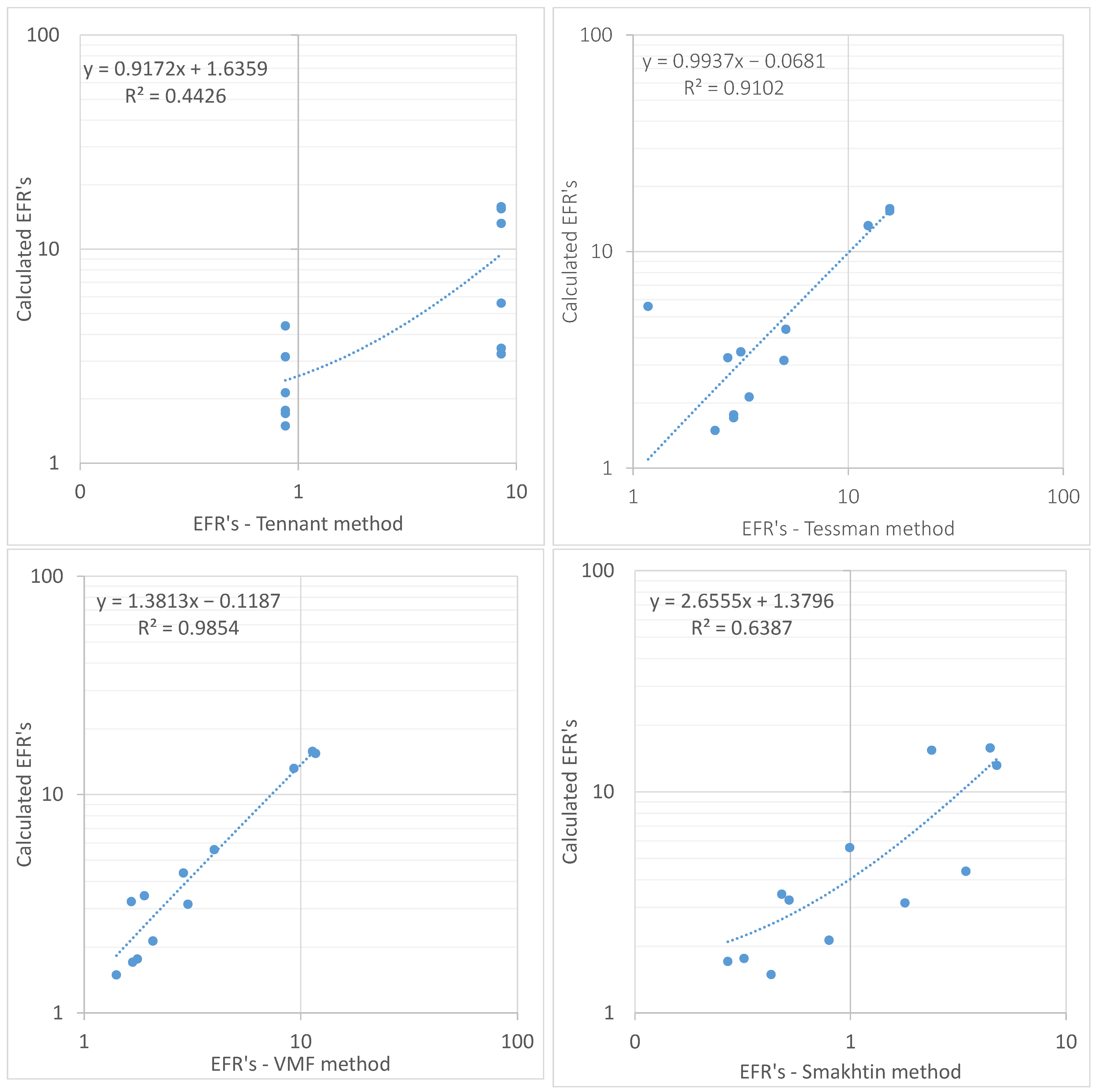
Figure 6 illustrates the correlation between the EFRs determined using the four different methods and the calculated EFR values. Results evidenced a very good correlation between the calculated EFR and the Tessman and the variable monthly flow (VMF) methods, with correlation coefficient (R²) values higher than 0.9. A good correlation was also identified for the Smakhtin method, which presented correlation coefficients of about 0.63. Finally, the lowest values were detected for the Tennant method with a R² lower than 0.5.

5. Conclusions and Discussion

In this study, the EFR was estimated using the Tennant, Tessman, variable monthly flow (VMF), and Smakhtin methods, starting from daily data measured in three-gauge stations (Ukai, Motinaroli, Ghala) in the lower reach of the Tapi River.

Generally, data on living organisms, the geometric data of the river, and real knowledge of the ecological effects of flow alternation are needed to correctly define EFs, but these data on the river ecosystem are not always available, an issue identified in past studies in the majority of the world’s river basins [18]. For this reason, the choice of EF methods for this study was limited to hydrological methods that were largely applied in past studies in which these methods were compared. For example, Hairan et al. [22] carried out a study on the evolution of the environmental flow of the Selangor River (Malaysia) using the hydrological index approach and the software Global Environmental Flow Calculator (GEFC). They analyzed daily flow data collected from Malaysia’s Department of Irrigation and Drainage (DID) over a 60-year period (1960–2020) and demonstrated that, from the overall comparison of the pre- and post-impact periods, the minimum flow in the dry seasons of the year increased, while the maximum flow decreased in the monsoon seasons during the post-impact period. Kumar et al. [23] applied three separate hydrological methodologies for EFA to calculate the minimal environmental flow requirements for the Srisailam dam (India) for the period 1968–2015. They identified that the reservoir operation policy was causing a severe hydrological alteration in the high flow season, especially in the month of July. Moreover, they concluded that in the case of the non-availability of environmental information, hydrological indicators can be used to provide the basic assessment of environmental flow requirements. Sahoo et al. [24] carried out an environmental assessment on the Mahanadi River Basin (India) by using the hydrological approach of environmental flow assessment. Using GEFC software, they evaluated the usefulness of numerous desktop hydrology-based environmental flow assessment methods such as Tennant, Tessman, variable monthly flow (VMF), range of variability approach (RVA), and FDC shifting methodology to evaluate environmental flows from daily discharge data.

Following these approaches, in this paper, the EFR values evaluated with the different methods were compared and, for each gauge station, the combination of the four methods, given by the average value of the EFR, was evaluated together with the low flow requirement (LFR) and the high flow requirement (HFR). Moreover, the results obtained with the four different methods were compared with the calculated EFRs in three different stations, also considering monthly variability, which indicates a significant improvement over previous studies based only on an annual scale [21,25]. Finally, the correlation between the EFRs determined using the four different methods and the calculated EFR values was investigated. In this study, the Tessman and the VMF methods gave the highest correlation with the calculated EFR. This result has also been evinced in past studies, such as that of Pastor et al. [18], in which these two methods showed good correlation with locally calculated EFRs in several case studies from a wide range of climates, flow regimes, and freshwater ecosystems. The timing and duration of low flows are critical to the health of the river ecosystem. In this context, the present study ensures the minimum value of flow necessary to maintain the sustainability of the watercourse. In any case, because of the lack of data on ecosystem response, the EF approaches in this study were limited to hydrological methods. In order to better define EFs, biological data, and river morphology data, an understanding of the ecological implications of flow alternation could be included in future studies and, thus, more information on ecological data should be gathered, as well as data from fisheries, as the timing and duration of low flows are essential to aquatic ecosystems’ health. Moreover, this study could be further improved by considering the whole Tapi River Basin.