Article

Intrinsic Characteristics of Forward Simulation Modeling Electric Vehicle for Energy Analysis

by
Christian Montaleza
1,
Paul Arévalo
1,2,*,
Marcos Tostado-Véliz
1 and
Francisco Jurado
1
1
Department of Electrical Engineering, Superior Polytechnic School of Linares, University of Jaén, 23700 Linares, Spain
2
Department of Electrical, Electronic and Telecommunications Engineering—DEET, Faculty of Engineering, University of Cuenca, Cuenca 010107, Ecuador
*
Author to whom correspondence should be addressed.
Electricity 2022, 3(2), 202-219; https://doi.org/10.3390/electricity3020012
Submission received: 27 April 2022 / Revised: 13 May 2022 / Accepted: 19 May 2022 / Published: 24 May 2022
(This article belongs to the Special Issue Recent Advances toward Carbon-Neutral Power System)

Abstract

:
The forward method for modeling electric vehicles is one of the most suitable for estimating energy consumption in different imposed driving cycles. However, a detailed description of the methodology used for the development of electric vehicle models is necessary and is scarce in the current literature. To fill this gap, this study focuses on highlighting the intrinsic characteristics through a theoretical study with a mathematical model, complemented by demonstrative simulations in Matlab/Simulink. The results show that the forward method can be estimated more accurately based on the energy consumption of the electric vehicle. Moreover, this paper aims to be explicitly descriptive for the development of more complex electric vehicle models to incorporate real driving cycles, being able to size the drivetrain of the vehicle itself or develop ecological routes.

1. Introduction

Numerical simulation based on mathematical modeling is a general method to evaluate the energy consumption of an electric vehicle (EV) on a certain route. The numerical methods are widely applicable, from statistical models to evaluate the CO2 emissions, kinematic models for the simulation of microscopic traces, or complex dynamic models to determine the influence of components [1]. There is a variety of computational tools that allow validation of the operation of EVs, focusing on responses to driving cycles [2]. The simulation process can be “backward” or “forward”, or even a combination between them. The former is relatively easier to use/implement, while the latter is more complex when adjusting to real driving cycles. Although there have been numerous studies that address the “forward” method for the development of EV models, these studies do not tackle a clear and concise description of the components involved in the development of models and estimate their energy consumption based on the imposed driving cycle. The study of the intrinsic characteristics of the forward method creates a starting point to develop computational models based on artificial neural networks (ANN), with the aim of determining the relationships between a series of factors that affect the energy consumption of EVs as a function of input parameters.
There is a wide variety of EV models available in the literature (e.g., see [3,4,5,6,7,8,9] and references therein), which, depending on the required detail of each component, can be stationary, quasi-stationary, or dynamic. Ref. [3] presents the modeling and simulation of a hybrid EV, while [4] focuses on the acoustic simulation of engines. In [5], the authors present a flat dynamic simulation of vehicles based on a real driving cycle. In [6,7], the modeling and estimation of the energy consumption of an EV is carried out, with rechargeable storage systems [6] and accurate EV energy model estimation [7]. Likewise, in [8,9], the authors focus on the modeling of high-performance powertrains, considering simulation and validation [8], as well as transmission parameters [9]. Most EV models can be stationary, quasi-stationary, or dynamic, depending on the detail required of each drivetrain component [10]. ADVISOR is a simulator developed by the National Renewable Energy Laboratory (NREL), which combines the backward and forward methods [11]. AUTONOMIE is a simulator developed by the Argonne National Laboratory (ANL), which uses the forward method [12,13]. Ref. [12] performs a validation model with dynamometer test data using AUTONOMIE, whereas [13] studies the life-cycle and greenhouse gas emissions resulting from different powertrain vehicles. These simulators simply allow data entry through a graphical interface, showing the results after simulating the model, without detailing the process for the development of EV models. Other studies use several software programs to adjust the model according to the results required [14], even extending to the public transport system, such as electric buses [15], to the energy management of powertrains [16], and to models of hybrid vehicles [17,18]. In [19], an integrated simulation of feed-forward hybrid EVs in Simulink and its use for energy management studies is presented. Similarly, the authors of [20] investigated the efficient performance of a hybrid with a variety of regenerative braking strategies. On the other hand, Ref. [21] presents a comparison between the forward and backward approaches for the simulation of an EV, while [22] carries out a comparative analysis between oriented forward and backward to rear-facing models in powertrain component sizing. However, there are no studies that show the methodology for developing an EV model based on the forward method, which is the method that best fits reality. Most of the existing literature focuses on presenting results of energy analysis based on models of EVs already performed or even by comparing this analysis with different simulation methods (backward or combined), i.e., the load state is compared at the end of the cycle, with EV emission modeling by the “forward” and “backward” methods. However, none of these models allow the identification of the involved components and the input variables to obtain a functional model by the “forward” method. To fill the gaps in the available literature, this study highlights all these intrinsic characteristics of the forward method. In addition, this study develops a model to estimate the state of charge (SOC) at the end of the driving cycle. This model aims at serving as a benchmark for analyzing more complex systems. In this regard, a theoretical study of the mathematical model of each of the components involved (e.g., driving cycle, driver model, powertrain, and multi-body vehicle model) is performed in this paper, thus serving to develop models of real driving cycles taken through a GPS with more precise and real results, as well as estimating the autonomy and energy consumption of the auxiliary elements of electric vehicles at all times. For simplicity, the main contributions of the present work are enumerated below:
  • Highlighting the intrinsic characteristics of the forward method;
  • Providing a systematic description of the blocks involved, together with their equations and necessary considerations for the development of the model;
  • Modeling, simulation, and validation of an electric vehicle by the forward method;
  • Energy analysis of the electric vehicle before an Urban Dynamometer Driving Schedule (UDDS) driving cycle.
The remainder of the paper is organized as follows: Section 2 presents the proposed materials and methods, including a mathematical representation of components using the forward method. Section 3 presents a case study with the results of the study. Finally, the main conclusions are duly drawn in Section 4.

2. Materials and Methods

The methodology used in this paper is schematically depicted in Figure 1. Firstly, the necessary background is presented, including a brief introduction to the forward method, which allows us to clearly identify its intrinsic characteristics. Next, this method is used to perform extensive simulations on a benchmark EV model, including the mathematical notations and model description in Matlab–Simulink, in order to demonstrate the consistency of the mathematical modeling.

2.1. Background

The backward simulation calculates the power demand of various components according to the driving cycle, to be posteriorly distributed among power sources in order to meet the vehicle’s demand. Finally, the energy consumption of the motor and batteries is obtained [16]. In contrast, in the forward simulation, the model determines the energy demand in the process of the driving cycle, to transmit the energy demand to the vehicle controller. This controller receives the signal and considers the current state of the vehicle components to optimize and determine power allocation, together with the output of each power source. The movement flow is transferred from the driving system, passing through the transmission to the tire module. Then, by means of equations that model the driving module, the real speed that is transmitted to the driver is calculated to form a closed cycle. Figure 2 represents a simple scheme of the simulation process by the “forward” method. The driving cycle provides the speed to pass through the driver model, which controls the longitudinal interfaces of the vehicle (accelerator and brake pedal), based on the difference between the object and the vehicle speed. The battery supplies the motor with energy and the motor provides a torque that, through the kinematic chain, transfers the movement to the wheels, where the traction maintains the propulsion force. The position returns to the driving cycle to find a target speed, closing the calculation loop.

2.2. Mathematical Modeling of the Forward Method

This section provides the mathematical foundations of the forward method, as well as the explanation of the blocks depicted in Figure 2.

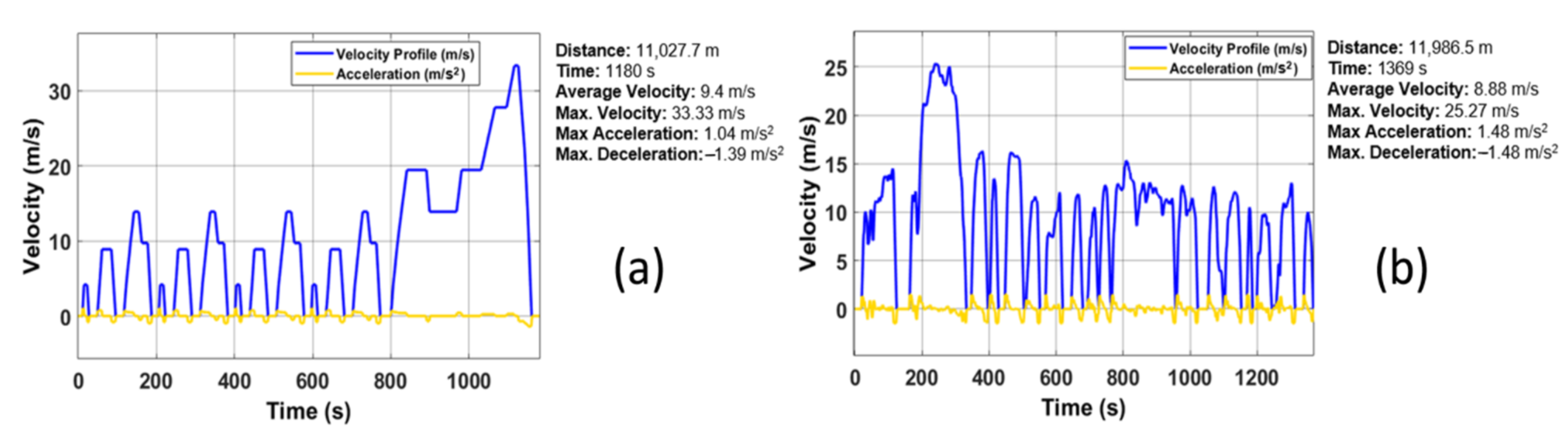
2.2.1. Driving Cycle Model

To estimate the SOC of on-board batteries and EV driving range, simulation models are based on internationally legislated driving cycles, and some represetative examples are as follows: Federal Test Procedure 72/75 (FTP 72/75), the New European Driving Cycle (NEDC) (see Figure 3a), the Japanese Cycle 08 (JC08), the Worldwide Harmonized Light Duty Cycle (WLTP), the 15-mode test cycle of the Economic Commission for Europe (ECE 15), and the UDDS (see Figure 3b), among many others. All of them differ in the sections of acceleration, braking, speed, cycle duration time, etc. [22,23,24,25,26].
In 2019, Europe adopted the WLTP as standard, thus rendering obsolete the NEDC. This cycle tests vehicles on longer routes, higher accelerations, and higher speeds; however, it is still believed that it does not fit reality. EVs are initially tested on a dynamometric bench in different driving cycles; one of the most important is the UDDS, which simulates driving in urban areas intermittently, starts the vehicle and accelerates it to the maximum speed allowed and stops it again. It is used to measure the energy consumption in the city. In the development of EV models for simulation, the UDDS cycle is conventionally used, by which the EV is subjected to multiple test cycles until the battery is completely discharged and stops by itself, thus providing preliminary autonomy. This study applies this driving cycle and not the obsolete NEDC cycle or the WLTP homologation cycle.

2.2.2. Driver Model

The controller module is suitable for the forward simulation model, by allowing the simulation model to form a closed-loop system, for which the PID controllers (Proportional, Integral, Derivative) are used, as observed in Figure 4. The forward method requires a driver model that acts as an accelerator/brake pedal actuator to follow the target speed (imposed driving cycle). For this, various controller models can be used; one of the most common is the PID controller, whose scheme is shown in Figure 4 [27]. The PID controller is based on repetitive tests and experience to determine the output values. The control system has a minimum static error between the actual simulation speed and the target speed; this error is necessary to maintain the torque of the drive wheels, because the changes in the simulation speed are always a function of the changes in the target speed [28]. If the PID parameters are properly calibrated, the delays will be slight and the motor drive torque is set efficiently; otherwise, the delays will be longer and could even cause a system discharge.
The transfer function of the PID controller is given by Equation (1).
k ( s ) = k p + k i s + k d s
where k p is the proportional coefficient, k i is the integral coefficient, and k d is the derivative coefficient.
In [29], the authors compared the conventional PID control with the linear square scheme (LQR), determining that LQR may outperform the conventional PID control. In particular, the scheme shown in Figure 5 was considered, taking values A = [1, 0, 2, 0], B = [1, 0], C = [0, 1], K = [12.2912, 31.6228], and gain for the entry step 31.6228 for the LQR. With these settings, it is observed in Figure 6 that the LQR controller improves the overshoot and settling time compared to the PID controller that takes values of P = 0.00012, I = 0.00047, and D = 0.000068 [30]. However, the PID controller has a shorter response time, being better behaved with fast speed transitions, maintaining a minimum error between the target and real speeds. On the basis of this conclusion, it is enough to apply a PID controller that performs the function of the pedal (acceleration/brake) to follow the target speed profile.

2.2.3. Brake Model

The braking force is proportional to the torque generated at the wheels. In order to stop the tire, a force must be applied that is contrary to the rotation movement, which is calculated in (2). In fact, Equation (2) calculates the necessary braking for just one wheel, it being necessary to multiply this result by the total number of wheels in order to obtain the necessary total braking force in the vehicle [31].
Braking   force   ( F F ) = N f r d
where N f is the braking torque (N), r d is the radius of the tire (m).
The ratio that determines the recoverable energy by means of regenerative braking is general and applies to any driving cycle [32]. The regenerative braking energy efficiency η rb is defined by Equation (3) [33,34].
η rb [ % ] = E recoverable [ kWh ] E available [ kWh ]  
where E recoverable [ kWh ] is the energy recovered during braking and E available [ kWh ] is the maximum energy available to be recovered during braking.
The available energy is calculated using Equation (4).
E avaliable [ kWh ] = 0 t P Wheels ( ) ( t )   dt          
where P Wheels ( - ) (t) is the negative part of the power in the wheels in [kW].

2.2.4. Electric Motor Model

The output power of the alternating current electric motor depends on its efficiency, which is modeled as a quasi-static efficiency map that depends on the output speed and torque, with the efficiency of the inverter considered constant. With these premises, the output power ( P em ) can be calculated by Equation (5) [35].
P em = min ( P inv · η em ( W em · T em ) · P inv η em ( W em · T em ) )        
where P inv is the power of the inverter (W), W em is the angular speed of the electric motor (rad/s), T em is the torque of the electric motor (Nm), and η em is the electric motor efficiency (%).
During simulation, the electric motor controller receives a power demand and adjusts the torque output to supply it. Since the current speed of the motor cannot change instantaneously, the theoretical torque is calculated by the controller based on the current speed of the motor and the power demand, and then finds the current efficiency of the motor from the efficiency map. However, it is also possible to resort to specific parameters of the electric motor by replacing the efficiency map with values of maximum torque and maximum power—see Equation (5)—and considering the motor loss constants ( k c , k i , and k w ) for the loss of power, power output is limited by the capacity of the electric motor, with the following equations:
P em   = T em · W em        
P loss   = k c · T em 2   +   k i · W + k w · W 3   + C
P in = T · W + P loss
P out     P max
P max   = P max ( W m )

2.2.5. Transmission Model

The drivetrain system transmits the movement obtained by the electric motor to the wheels as shown in Figure 7, which is modeled by (11) and (12).
T el em = r d η g · G · F t
T em el   =   η g · ( r d G · F t )
where η g is the transmission efficiency (%), F t is the pulling force (N), G is the transmission ratio [36].
Equation (11) is used when the electric motor is delivering mechanical power ( T el - em ) and Equation (12) is used when the electric motor is receiving mechanical power ( T em - el ) [37]. Likewise, the relationship between the linear speed “v” of the electric vehicle and the angular speed Wem of the motor in (rad/s) can be obtained by Equation (13).
W em = G v r d
Finally, the transmission force is obtained with Equation (14).
F tr = ( T em   T Loss ) · G r d   F Tf
where T Loss is the friction losses associated with the torque.

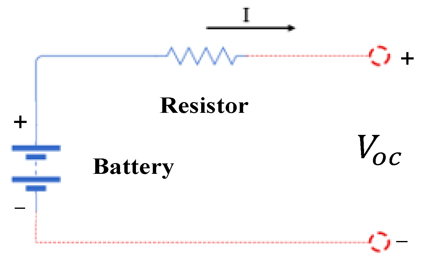
2.2.6. Battery Model

The battery modeling can be addressed in various ways, the most used being the electric and physical electrochemical models [38,39]. The equivalent electrical model is simple to build and adjust, giving good results in estimating voltage, current, SOC, and heat rate [40]. On the other hand, it is possible to express the physical model of the battery based on electrochemical phenomena. However, this method can be complex and computationally expensive, and is also commonly used to evaluate its behavior outside the predetermined temperature range of the batteries. Another key aspect of this modeling is the ability to use models of physics-based (as opposed to empirical) aging that give insight into the growth rate of the cathode film, the lithium coating, and the insulation of the material due to cracking [41,42]. In summary, the objective is to estimate the energy consumption of the EV throughout a driving cycle but not to estimate the aging of each battery cell or the degradation of the performance of the system over time. Thus, it could be more feasible to use the equivalent electrical model for battery [43]. Through the equivalent electrical model, this type of charging and discharging behavior is represented in an electrical circuit using the resistive battery model, as shown in Figure 8. The battery model in the simulation is not subjected to a deep discharge (below 20%) nor until all energy is exhausted (0%); it is only subjected to the analysis of the state of charge at the end of the UDDS cycle.
The maximum battery power denoted by pmax points out the maximum power that the storage set can exchange with the system, and is given by Equation (15).
pmax = V ve V oc   V ve R int
where V oc is the open circuit voltage (V), V ve is the minimum motor controller voltage or the minimum battery voltage, and R int is the charge and discharge resistance. The charge or discharge current is calculated with Equation (16).
I = V oc   V oc 2   4 R int · P 2 R int
where P is the charging/discharging power of the batteries. The SOC of the batteries can be estimated using Equation (17).
SOC = Ah max     Ah used Ah max
where Ah max is the maximum capacity of the battery bank and Ah used is the used capacity of the battery bank.

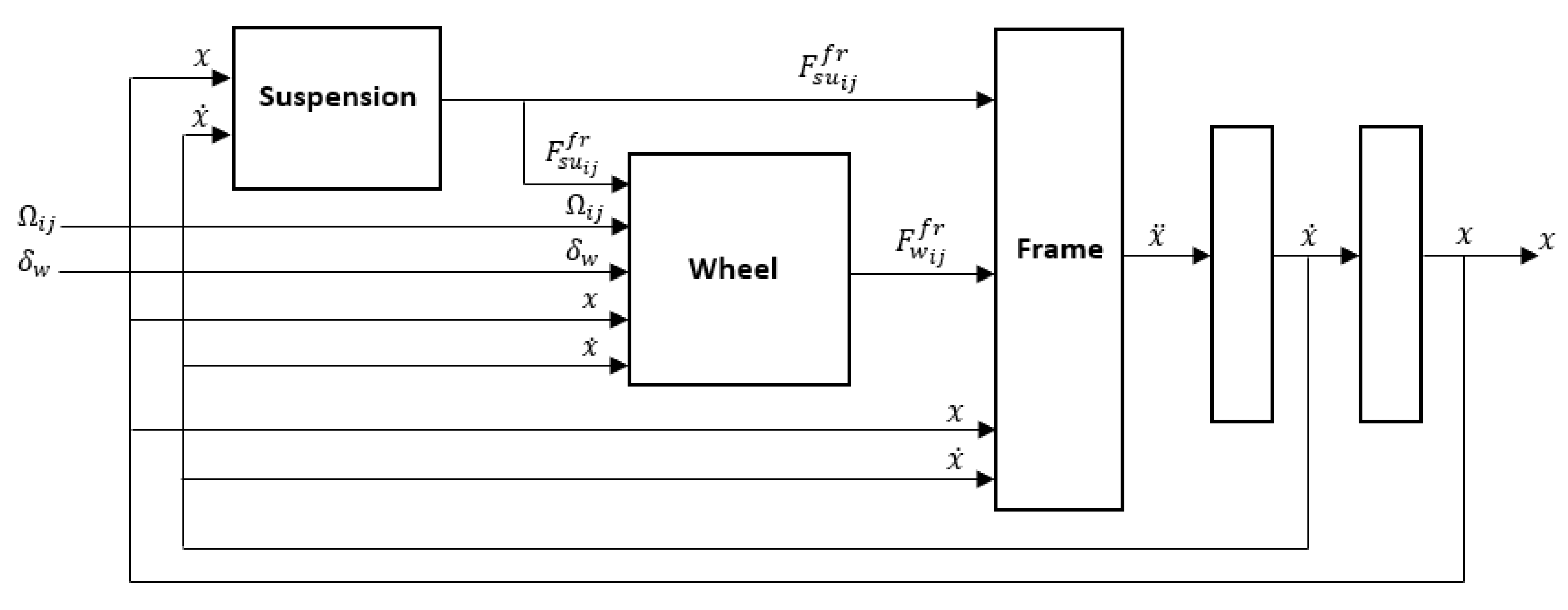
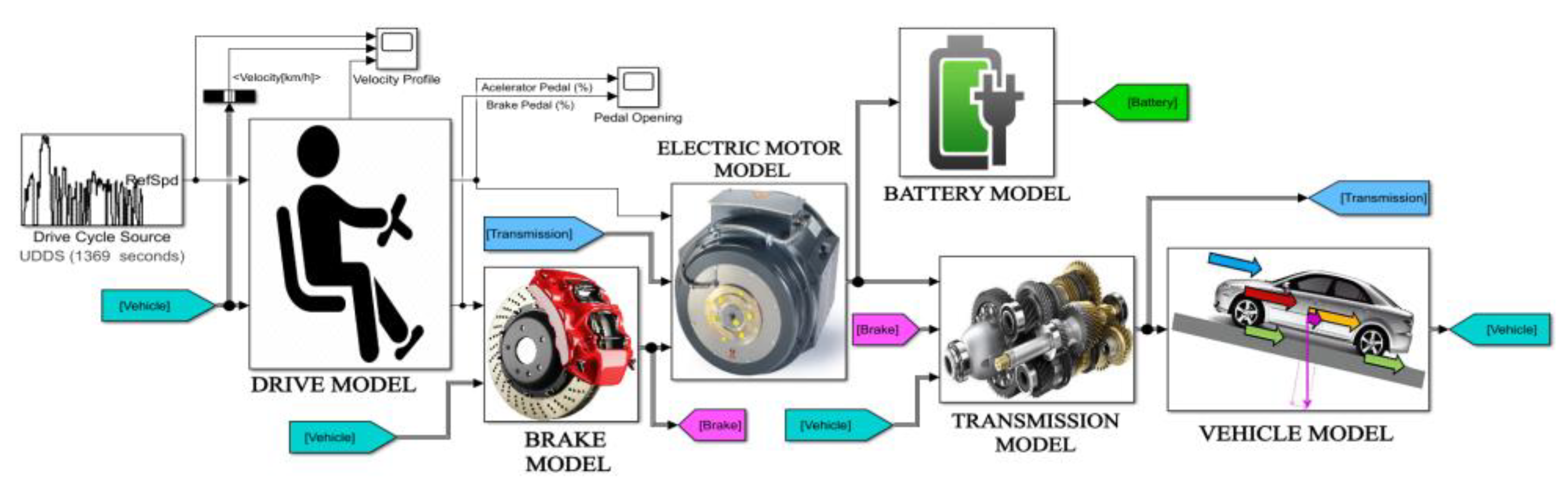
2.2.7. EV Global Model

Longitudinal Dynamics
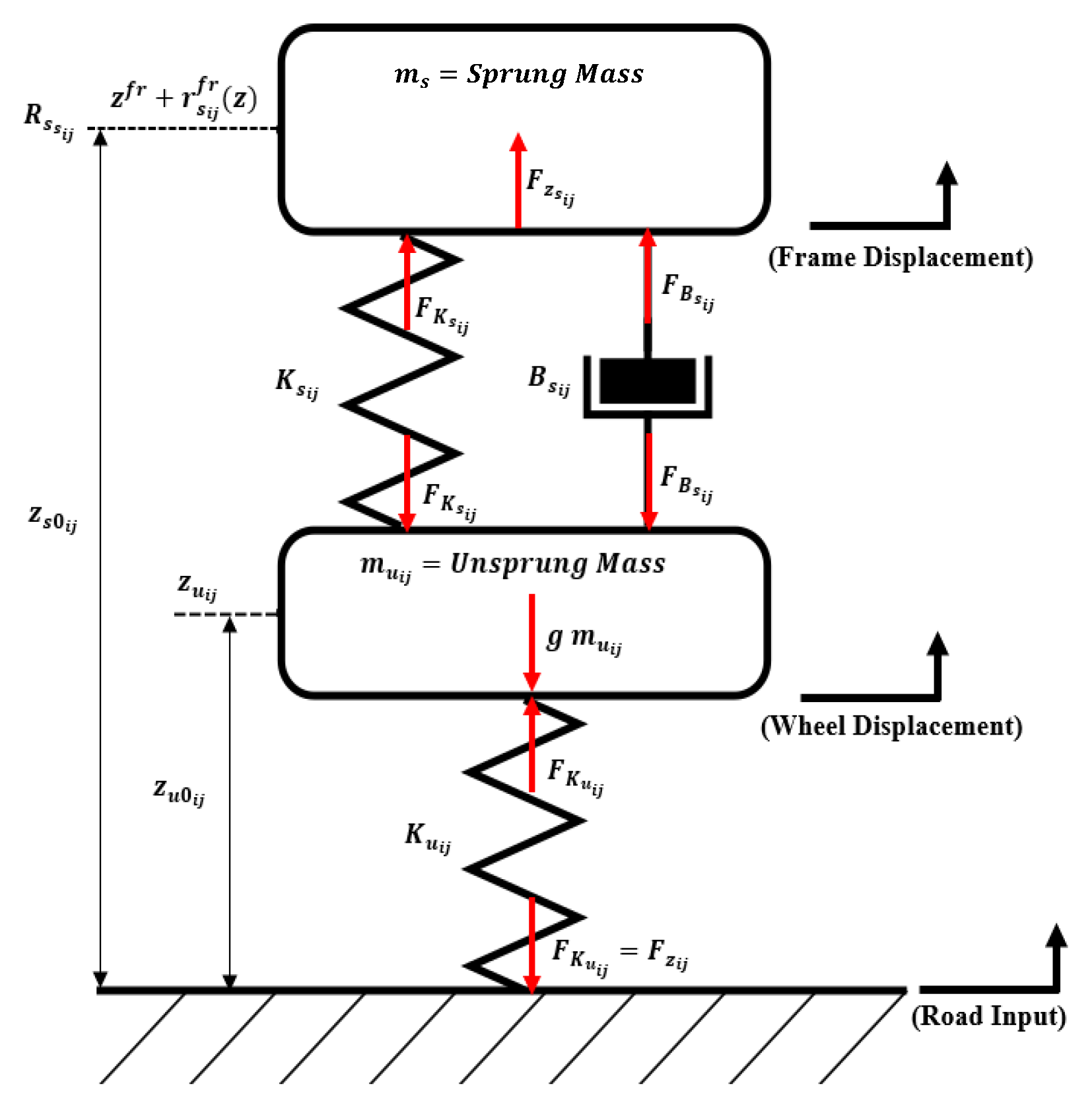
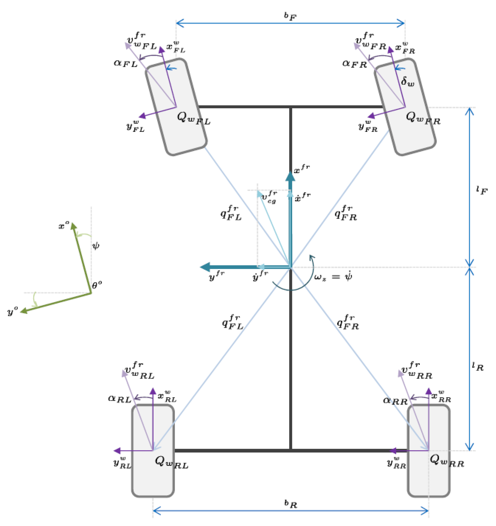
For EV modeling, the inertia and resistances of the vehicle must be represented. Longitudinal dynamics analyzes the behavior of the vehicle when it is subjected to speed fluctuations in the longitudinal plane, neglecting the lateral acceleration [44]. In this case, the vehicle moves in a straight line, accelerating, braking, or changing the slope. Longitudinal dynamics is affected by different resistances, such as rolling, aerodynamics, and slope resistance [45]. To analyze these factors, a vehicle moving on an inclined plane and in a straight line is considered.
The aerodynamic drag is a force acting on objects moving in a fluid opposite to their motions, which is calculated with Equation (18) [27].
F a = 1 2 ρ · A · C d · v 2
where ρ is the density of air, A is the frontal area of the EV, C d is the drag coefficient that depends on the shape of the vehicle for a particular vehicle C d and varies between 0.3 and 0.4, and v is the speed of the EV.
Two other parameters are of importance when modeling the longitudinal dynamics: the rolling and slope resistance. The first coefficient refers to the resistance force of the rotational movement of the tire in contact with the surface, which is denoted by F rr and can be calculated with Equation (19), while the slope resistance is denoted by F rp and is given by (20). Finally, it is worth mentioning that the pulling force F t is given by (21) [27,46].
F rr = m · g · C r · cos θ
F rp = m · g · sin θ
F t = m · a + m · g · C r · cos θ   +   1 2 ρ · A · C d · v 2 + m · g · sin θ
where m is the mass of the EV, g is the gravity acceleration, C r is the coefficient of friction, θ is the angle of inclination between the EV and the surface, and a is the acceleration of the EV.

Multibody

In this section, the multibody modeling that represents each individual component of the EV based on their lateral and vertical physical properties is analyzed. Three degrees of freedom are considered for this theoretical study; however, it is worth mentioning that other, more sophisticated models can represent up to 94 degrees [47]. To express the complete block of the multibody, in this paper, the mathematical models of the vehicle frame, suspension, and wheels are considered.
The frame vehicle is modeled as a rigid body on which the translational displacement in the three directions of the fixed coordinate system ( x ,   y ,   z ) and the rotary movement around the three axes ( φ ,   χ ,   ψ ) are represented, in order to obtain the output vector X = [ x   y   z   φ   χ   ψ ] T . These movements occur due to the effect of rolling resistance ( F R ij fr ) , tire forces ( F x ij fr ,   F y ij fr ) , and tire forces on the frame suspension ( F Zs ij fr )   [48]. For the calculation of the angular displacement, Euler’s Law is applied. In addition, the angular accelerations of the vehicle can be obtained through the centroidal inertia matrix and the moments exerted by the forces on the body [49]. To obtain the angular accelerations of EV ( w p ) , Equation (22) is applied.
w p = E · [ φ · χ · ψ · ]   + E [ φ ¨ χ ¨ ψ ¨ ]  
where E · is the Euler derivate function, φ represents the rotation on the x-axis, χ represents the rotation on the y-axis, and ψ represents the rotation on the z-axis.
For the suspension model, the position vectors r s ij cg must initially be established for each vertex R s ij with respect to the coordinate system of the center of gravity, with the aim of determining the overall displacement, as shown in Figure 9. The reaction force of the suspension on the frame can be calculated by using Equation (23).
F z s ij = F K s ij +   F B s ij K s ij ( dz u ij   -   dz s ij ) + B s ij [ Z · u ij - ( Z · + r s ij o ( z ) ) ]
Finally, the mathematical modeling of the wheels complements the multibody model. In this sense, the behavior of the wheels significantly affects the performance of the vehicle due to the horizontal forces and moments generated [50]. In addition, the wheels support other types of efforts by having to hold up the weight of the vehicle, as well as the forces of aerodynamic load and mass transfer during braking or turning of the vehicle [49]. Experimental methods are used to simplify and model the tire. One of the most used and well-known is the Pacejka model. This model relates the longitudinal force ( F x ) , the lateral force F y , and the alignment moment ( M z ) with the drift angle ( α ) and the drift ratio ( κ ) of the wheels by means of a set of formulas to interpolate all data. First, the centers of rotation of the wheels ( Q i j ) are defined in the horizontal plane with respect to the origin of the frame coordinate system by means of the position vectors q i j f r . Figure 10 details the dimensions of the vehicle [50].
Lastly, it is necessary to rotate the horizontal forces of the front wheels by the angle of twist δw around the z-axis, as shown in Equation (24). To sum up, the different sub-blocks involved in EV modeling are depicted in Figure 11, for simplicity.
[ F xij fr F yij fr 0 ] = R w fr ( δ w ) [ F xij w F yij w 0 ]
where F su ij fr represents the position vector of each component applied from the suspension on the chassis and the wheel, respectively, F w ij fr represents the position vector of each component applied from the wheels on the chassis, and Ω i j is the angular velocity of the wheels.

2.3. Simulation

A modeling of the EV is developed with the forward method approach (Figure 12), which comprises all the blocks described throughout the study, using longitudinal dynamics for vehicle modeling. The cycle used is the UDDS (see Figure 3b) and the input values are collected in Table 1.

3. Results and Discussion

This section presents the results and discussion of the simulations performed on Matlab–Simulink, in which all the parameters and forces interacting on the EV and the energy of the vehicle at the end of the imposed driving cycle can be estimated, as observed in Figure 13. The EV profile is similar to the UDDS route, which is passed to the driver model. The PID controller converts the error into signals for the accelerator and brake pedal. Therefore, its representation is observed in detail throughout the driving cycle, as seen in Figure 14. Figure 15 shows the SOC of the battery bank throughout the driving cycle. The initial state of charge was considered equal to 80.7% and, after completing the route (1369 s), declined to 74.3%, being therefore reduced by 6.4%. Figure 16 shows the battery voltage variation thorughout the driving cycle. The average voltage required is 340 V, with the maximum capacity of the battery being 350 V, a capacity that is not exceeded during the driving cycle.
Figure 17 shows the battery current variation thorughout the route. The average current required is 50 A; the current is proportional to the speed, and if the speed increases, more current is demanded. In Figure 18, a comparison of the variation in the speed and the variation in the battery power is shown. It can be seen that the velocity changes are proportional to the battery power. Table 2 shows the energy results of the EV using the method proposed for the UDDS cycle; for a distance of approximately 12 km, the battery has been discharged by almost 25%.
Undoubtedly, this is a method used by many studies for the modeling and simulation of an EV for charging and discharging estimation throughout the driving cycle. This study focuses on the model development process in general, and not on developing each component in its complex form, as in Ref. [35], where electric motors are designed and analyzed for applications in plug-in EVs, or in [51,52], where the regenerative brake is studied and modeled. Similarly, in Ref. [53], the authors model other complementary and important components, such as the converter DC/DC and inverter. After understanding the process of forward modeling, it is possible to include it in the integral simulation chain, replacing the basic components, including energy management systems, by analyzing the effect of temperature on a system’s energy storage [54]; thus, it will be possible to obtain more accurate and realistic estimates.
The multibody modeling of the vehicle in the actual literature is neglected, not providing much difference compared to the longitudinal modeling, when estimating the energy consumption. The multibody modeling of the vehicle depends on the results that are required; on the other hand, this modeling is ideal for analyzing the dynamic performance of each component (suspension, chassis, and tire) and even for analyzing the lateral behavior of the steering system. The multibody modeling involves sub-models that depend on the degrees of freedom, its modeling being much more complex. In Ref. [47], the authors analyze a model with 94 degrees of freedom. Longitudinal dynamics is favorable for estimating energy consumption, because it can include a slope profile together with the speed profile to be input parameters to the driver’s model, and it can also incorporate the consumption of auxiliary elements of the EV, such as electric motors for the steering system, air conditioning, pumps, etc.
When comparing the characteristics of the backward and forward methods, a peculiarity of the latter stands out, since the acceleration of the vehicle is expressed as a function of the accelerator position, unlike the backward method, where the force required to accelerate the vehicle is determined only from the speed cycle. For this reason, the forward method is a more complex and accurate method, which serves to develop real-time eco-driving systems and eco-routes that can improve energy efficiency to extend the EV’s travel range, as studied in [43]. Table 3 compares autonomy with the simulation of a more accurate model from the Matlab/Simulink library, adjusting the input values of Table 1, and also with [14], a reference used for the validation of the model.
The model developed in this study has higher energy consumption per hour than the Matlab models and [14]. These EV models (Matlab, Ref. [14]) are more complex and apply control algorithms for the drivetrain and for battery energy management; it incorporates components such as BMS, sensors, regenerative braking, etc., leading to greater accuracy in estimating energy consumption. The battery charge status for the EV model from the matlab/simulink library is shown in Figure 19 and for the EV model from [14] it is shown in Figure 20. The three models are developed by the same method (forward), but there is a large difference in energy consumption, especially in the model developed in this study. It should be noted that this study focuses on highlighting the development process of the EV model by the forward method, but not on developing a model that improves consumption autonomy. For the estimation of autonomy, values from the United States Environmental Protection Agency (US EPA) are used.

4. Conclusions

A detailed study of the modeling and simulation of the EV is presented considering the forward method for its development, highlighting the intrinsic characteristics. One of the aspects that clearly differs compared to the backward method is the model of the driver, who acts as an acceleration and braking pedal to follow the imposed target speed. Driver modeling can be achieved by different controllers: the classic PID, Pole Location Controller, Linear Quadratic Regulator (LQR), and Observer Based Controller (OBC). LQR is one of the controllers that best adjusts the throttle position; therefore, it is compared with the PID controller, looking at their response time to a simple step. The LQR controller improves the overshoot, while properly adjusting the PID controller reduces the response and stabilization time; for this study, a PID controller is used, where the results do not show a greater error between the target speed and the real speed of the vehicle. The use of one controller or another depends on the results required and the type of vehicle.
The results of the forward method can estimate the energy consumption of the EV, as well as the energy losses in the components. In this particular case, the input data (Table 2) were obtained as a result after fulfilling the driving cycle UDDS 1396 s, with a distance traveled of 11.99 km. The SOC dropped from 80.7% to 74.3%, with energy consumption of 2209 kWh and energy losses in some components, such as the electric motor, of 0.429 kWh, the transmission of 0.221 kWh, and the battery of 0.0324 kWh.
The simulation was also compared with other more precise models (Table 3); one of them was an existing model in the Matlab library (Powertrain Blockset version 1.10), and we also compared it with the reference [14], which uses the AUTONOMIE simulator. For all of them, the same values are adjusted. From the outset, where there is a notable difference is in the autonomy; the model developed in this study consumes more energy, having an autonomy of 4.45 kWh/100 km, and the one that consumes the least is the one that uses the AUTONOMIE simulator, with a consumption of 0.97 kWh/100 km.
Future research can focus on these concepts to develop computational models based on artificial neural networks (ANN) to determine the relationships between a series of factors that affect the energy consumption of EVs depending on the input factors, where it is determined a weight for each factor based on its relative importance using training algorithms. ANN can also be used to predict driving behavior by classifying driving patterns using Global Positioning System data, being an extremely important approach method as it is data-driven and self-adaptive.

Author Contributions

Conceptualization, C.M.; Data curation, C.M.; Formal analysis, C.M.; Funding acquisition, F.J.; Investigation, C.M.; Methodology, P.A.; Project administration, F.J.; Resources, P.A.; Software, P.A.; Supervision, M.T.-V. and F.J.; Validation, M.T.-V.; Visualization, M.T.-V.; Writing—original draft, P.A.; Writing—review and editing, P.A. All authors have read and agreed to the published version of the manuscript.

Funding

This research received no external funding.

Institutional Review Board Statement

Not applicable.

Informed Consent Statement

Not applicable.

Data Availability Statement

Not applicable.

Acknowledgments

This paper was supported by the Ibero-American Postgraduate University Association (AUIP) through the Academic Mobility Program between Andalusian and Ibero-American universities 2020.

Conflicts of Interest

The authors declare no conflict of interest.

References

  1. Pettersson, P.; Jacobson, B.; Bruzelius, F.; Johannesson, P.; Fast, L. Intrinsic differences between backward and forward vehicle simulation models. IFAC PappersOnLine 2020, 53, 14292–14299. [Google Scholar] [CrossRef]
  2. Ibrahim, A.; Jiang, F. The electric vehicle energy management: An overview of the energy system and related modeling and simulation. Renew. Sustain. Energy Rev. 2021, 144, 111049. [Google Scholar] [CrossRef]
  3. Gao, D.W.; Mi, C.; Emandi, A. Modeling and Simulation of Electric and Hybrid Vehicles. Proc. IEEE 2007, 95, 729–745. [Google Scholar] [CrossRef]
  4. Li, H.; Xu, P.; Cao, C.; Hu, D.; Yan, X.; Song, Z. Acoustic Simulation of the Electric Vehicle Motor. J. Phys. Conf. Ser. 2021, 2095, 12031. [Google Scholar] [CrossRef]
  5. Miranda, M.; Silva, F.; Lourenço, M.; Eckert, J.; Silva, L. Electric vehicle powertrain and fuzzy controller optimization using a planar dynamics simulation based on a real-world driving cycle. Energy 2022, 238, 121979. [Google Scholar] [CrossRef]
  6. Aymen, F.; Alowaidi, M.; Bajaj, M.; Sharma, N.; Mishra, S.; Sharma, S.K. Electric Vehicle Model Based on Multiple Recharge System and a Particular Traction Motor Conception. IEEE Access 2021, 9, 49308–49324. [Google Scholar] [CrossRef]
  7. Miri, I.; Fotouhi, A.; Ewin, N. Electric vehicle energy consumption modelling and estimation—A case study. Int. J. Energy Res. 2021, 45, 501–520. [Google Scholar] [CrossRef]
  8. Adegbohun, F.; Von Jouanne, A.; Phillips, B.; Agamloh, E.; Yokochi, A. High Performance Electric Vehicle Powertrain Modeling, Simulation and Validation. Energies 2021, 14, 1493. [Google Scholar] [CrossRef]
  9. Yaxin, G.; Yi, F. Transmission Parameter Matching and Simulation Verification of Pure Electric Vehicle. J. Phys. Conf. Ser. 2021, 1965, 12015. [Google Scholar] [CrossRef]
  10. Chen, L.; Li, Z.; Yang, J.; Song, Y. Lateral Stability Control of Four-Wheel-Drive Electric Vehicle Based on Coordinated Control of Torque Distribution and ESP Differential Braking. Actuators 2021, 10, 135. [Google Scholar] [CrossRef]
  11. Wipke, K.B.; Cuddy, M.R.; Burch, S.D. ADVISOR 2.1: A user-friendly advanced powertrain simulation using a combined backward/forward approach. IEEE Trans. Veh. Technol. 1999, 48, 1751–1761. [Google Scholar] [CrossRef]
  12. Kim, N.; Douba, M.; Kim, N.; Rousseau, A. Validation Volt PHEV Model with dynamometer test data using Autonomie. SAE Int. J. Passeng. Cars Mech. Syst. 2013, 6, 985–992. [Google Scholar] [CrossRef]
  13. Lewis, A.M.; Kelly, J.C.; Keoleian, G.A. Vehicle lightweighting vs. electrification: Life cycle energy and GHC emissions results for diverse powertrain vehicles. Appl. Energy 2014, 126, 13–20. [Google Scholar] [CrossRef]
  14. Lee, D.; Rousseau, A.; Rask, E. Development and Validation of the Ford Focus Battery Electric vehicle model. SAE Tech. Pap. 2014, 1, 1–9. [Google Scholar] [CrossRef]
  15. Hou, J.; Guo, X. Modeling and Simulation of hybrid electric vehicles using HEVSIM and ADVISOR. In Proceedings of the IEEE Vehicle Power and Propulsion Conference, Harbin, China, 3–5 September 2008. [Google Scholar] [CrossRef]
  16. Jiang, C.D.; Cheng, L.; Fengchun, S. Study on forward simulation model for extended-range electric bus. In Proceedings of the Third World Congress on Software Engineering, Wuhan, China, 6–8 November 2012. [Google Scholar] [CrossRef]
  17. He, Y.; Rios, J.; Chowdhury, M.; Pisu, P.; Bhavsar, P. Forward powertrain energy management modeling for assessing benefits of integrating predictive traffic data into plug-in-hybrid electric vehicles. Transp. Res. Part D Transp. Environ. 2012, 17, 201–207. [Google Scholar] [CrossRef]
  18. Lin, C.; Filipi, Z.; Wang, Y.; Louca, L.; Peng, H.; Assanis, D.; Stein, J. Integrated, Feed-Forward Hybrid Electric Vehicle Simulation in SIMULINK and its Use for Power Management Studies. SAE Tech. Pap. 2002, 1, 1–15. [Google Scholar] [CrossRef]
  19. Qin, D.; Deng, T.; Yang, Y.; Lin, Z. Regenerative braking simulation research for CVT hybrid electric vehicle with ISG based on forward modeling. Electr. Eng. 2008, 19, 618–624. [Google Scholar]
  20. Delavaux, M.; Lhomme, W.; Mcgordon, A. Comparison between Forward and Backward approaches for the simulation of an Electric Vehicle. In Proceedings of the IEEE Vehicle Power and Propulsion Conference, Lille, France, 3–5 September 2010. [Google Scholar]
  21. Mohan, G.; Assadian, F.; Longo, S. Comparative analysis of forward-facing models vs. backward-facing models in powertrain component sizing. In Proceedings of the IET Hybrid and Electric Vehicles Conference, London, UK, 6–7 November 2013. [Google Scholar] [CrossRef] [Green Version]
  22. Zhao, X.; Zhao, X.; Yu, Q.; Ye, Y.; Yu, M. Development of a representative urban driving cycle construction methodology for electric vehicles: A case study in Xi’an. Transp. Res. Part D Transp. Environ. 2020, 81, 102279–102301. [Google Scholar] [CrossRef]
  23. Kurnia, J.C.; Sasmito, A.P.; Shamim, T. Performance evaluation of a PEM fuel cell stack with variable inlet flows under simulated driving cycle conditions. Appl. Energy 2017, 206, 751–764. [Google Scholar] [CrossRef]
  24. Seers, P.; Nachin, G.; Glaus, M. Development of two driving cycles for utility vehicles. Transp. Res. Part D Transp. Environ. 2015, 41, 377–385. [Google Scholar] [CrossRef]
  25. Yuhui, P.; Yuan, Z.; Huibao, Y. Development of a representative driving cycle of urban buses based on the K-means cluster method. Clust. Comput. 2019, 22, 6871–6880. [Google Scholar] [CrossRef]
  26. Ye, K.; Li, P.; Li, H. Optimization of hybrid energy storage system control strategy for pure electric vehicle based on typical driving cycle. Math. Probl. Eng. 2020, 2020, 1365195–1365207. [Google Scholar] [CrossRef]
  27. Kiyakli, A.O.; Solmaz, H. Modeling of an electric vehicle with Matlab/Simulink. Int. J. Automot. Sci. Technol. 2019, 2, 9–15. [Google Scholar] [CrossRef]
  28. Ali, R.; Furqan, A.; Ho, K.S. Design of fuzzy logic tuned PID controller for electric vehicle based on IPMSM using Fluxweakenning. J. Electr. Eng. Technol. 2018, 13, 451–459. [Google Scholar] [CrossRef]
  29. Saeed, M.; Ahmed, N.; Hussain, M.; Jafar, A. A comparative study of controllers for optimal speed control of hybrid electric vehicle. In Proceedings of the International Conference on Intelligent Systems Engineering, Islamabad, Pakistan, 15–17 January 2016. [Google Scholar] [CrossRef]
  30. Heidari, A.; Etedali, S.; Javaheri-Tafti, M. A hybrid LQR-PID control design for seismic control of buildings equipped with ATMD. Front. Struct. Civ. Eng. 2018, 12, 44–57. [Google Scholar] [CrossRef]
  31. Ma, Z. Parameters design for a parallel hybrid electric bus using regenerative brake model. Adv. Mech. Eng. 2014, 6, 760815–760824. [Google Scholar] [CrossRef]
  32. Bin Peeie, H.M.; Ogino, H.; Oshinoya, Y. Skid control of a small electric vehicle with two in-wheel motors: Simulation model of ABS and regenerative brake control. Int. J. Crasheorthiness 2016, 21, 396–406. [Google Scholar] [CrossRef] [Green Version]
  33. Liu, Z.; Ortmann, W.J.; Nefcy, B.; Colvin, D.; Connolly, F. Methods of measuring regenerative braking efficiency in a test cycle. SAE Int. J. Altern. Powertrains 2017, 6, 103–112. [Google Scholar] [CrossRef]
  34. Zhu, Y.; Wu, H.; Zhen, C. Regenerative braking control under sliding braking condition of electric vehicles with switched reluctance motor drive system. Energy 2021, 230, 120901. [Google Scholar] [CrossRef]
  35. Yilmaz, M. Limitations/capabilities of a electric machine technologies and modeling approaches for electric motor design and analysis in plug-in electric vehicle applications. Renew. Sustain. Energy Rev. 2015, 52, 80–99. [Google Scholar] [CrossRef]
  36. Park, G.; Lee, S.; Jin, S.; Kwak, S. Integrated modeling and analysis of dynamics for electric vehicle powertrains. Expert Syst. Appl. 2014, 41, 2595–2607. [Google Scholar] [CrossRef]
  37. Fajri, P.; Lee, S.; Prabhala, V.A.; Ferdowsi, M. Modeling and Integration of electric vehicle regenerative and friction braking for motor/dynamometer test bench emulation. IEEE Trans. Veh. Technol. 2016, 65, 4264–4273. [Google Scholar] [CrossRef]
  38. Wang, Y.; Tian, J.; Sun, Z.; Wang, L.; Xu, R.; Li, M.; Chen, Z. A comprehensive review of battery modeling and state estimation approaches for advanced battery management systems. Renew. Sustain. Energy Rev. 2020, 131, 100015–110033. [Google Scholar] [CrossRef]
  39. Meng, J.; Luo, G.; Ricco, M.; Swiercynski, M.; Stroe, D.I.; Teodorescu, R. Overview of lithium-ion battery modeling methods for state-of-charge estimation in electrical vehicles. Appl. Sci. 2018, 8, 659. [Google Scholar] [CrossRef] [Green Version]
  40. Seaman, A.; Dao, T.S.; McPhee, J. A survey of mathematics based equivalent circuit and electrochemical battery models for hybrid and electric vehicle simulation. J. Power Sources 2014, 256, 410–423. [Google Scholar] [CrossRef] [Green Version]
  41. Li, J.; Wang, D.; Deng, L.; Cui, Z.; Lyu, C.; Wang, L.; Pecht, M. Aging modes analysis and physical parameter identification based on a simplified electrochemical model for lithium-ion batteries. J. Energy Storage 2020, 31, 101538–101551. [Google Scholar] [CrossRef]
  42. Choi, W.; Shin, H.C.; Kim, H.C.; Choi, J.Y.; Yoon, W.S. Modeling and applications of electrochemical impedance spectroscopy (Eis) for lithium-ion batteries. J. Electrochem. Sci. Technol. 2020, 11, 1–13. [Google Scholar] [CrossRef] [Green Version]
  43. Abdollahi, A.; Han, X.; Raghunathan, N.; Pattipati, B.; Balasingam, B.; Pattipati, K.R.; Bar-Shalom, Y.; Card, B. Optimal charging for general equivalent electrical battery model and battery life management. J. Energy Storage 2017, 9, 47–58. [Google Scholar] [CrossRef] [Green Version]
  44. Da Lio, M.; Bortoluzzi, D.; Pietro Rosati Papini, G. Modeling longitudinal vehicle dynamics with neural networks. Veh. Syst. Dyn. 2020, 58, 1675–1693. [Google Scholar] [CrossRef] [Green Version]
  45. Esmailzadeh, E.; Vossoughi, C.R.; Goodarzi, A. Dynamic modeling and analysis of a four motorized wheels electric vehicle. Veh. Syst. Dyn. 2001, 35, 163–194. [Google Scholar] [CrossRef]
  46. Juhala, M. Improving vehicle rolling resistance and aerodynamics. In Alternative Fuels and Advances Vehicle Technologies for Improved Environmental Performance; Folkson, R., Ed.; Woodhead Publishing: Cambridge, UK, 2014; pp. 462–475. [Google Scholar]
  47. Hegazy, S.; Rahnejat, H.; Hussain, K. Multi-body dynamics in full vehicle handling analysis. Proc. Inst. Mech. Eng. Part K. J. Multi-Body Dyn. 1999, 213, 19–31. [Google Scholar] [CrossRef] [Green Version]
  48. Blundell, M.; Harty, D. The Multibody System Approach to Vehicle Dynamics, 2nd ed.; Elsevier Butterworth Heinemann: New York, NY, USA, 2004; Volume 1, pp. 30–160. [Google Scholar]
  49. Lo, R.; Massaro, M.A. Symbolic approach to the multibody modeling of road vehicles. Int. J. Appl. Mech. 2017, 9, 17500685. [Google Scholar] [CrossRef]
  50. Milliken, M.F.; Milliken, D.L. Race Car Vehicle Dynamic, 2nd ed.; Society of Automotive Engineers: Warrendale, PA, USA, 1994. [Google Scholar]
  51. Wang, J.; Qiao, J.; Qi, Z. Research on control strategy of regenerative braking and anti-lock braking system for electric vehicle. In Proceedings of the World Electric Vehicle Symposium and Exhibition (EVS27), Barcelona, Spain, 1–7 November 2013. [Google Scholar] [CrossRef]
  52. Yu, C.; Shim, T. Modeling of comprehensive electric drive system for a study of regenerative brake system. In Proceedings of the American Control Conference, Washington, DC, USA, 17–19 June 2013. [Google Scholar] [CrossRef]
  53. Moreno, P.; Blanco, M.; Lafoz, M.; Arribas, J.R. Educational Project for the teaching of control of electric traction drives. Energies 2015, 8, 921–938. [Google Scholar] [CrossRef] [Green Version]
  54. Rahimirad, P.; Masih-Tehrani, M.; Dahmardeh, M. Battery life investigation of a hybrid energy management system considering battery temperature effect. Int. J. Automot. Eng. 2019, 9, 2966–2976. [Google Scholar]
Figure 1. Schematic explanation of the proposed methodology.
Electricity 03 00012 g001
Figure 2. Schematic representation of the forward simulation process.
Electricity 03 00012 g002
Figure 3. Examples of standard driving cycles: NEDC (a) and UDDS (b).
Electricity 03 00012 g003
Figure 4. PID controller.
Electricity 03 00012 g004
Figure 5. Scheme for the simulation of the PID and LQR controller.
Electricity 03 00012 g005
Figure 6. Simulation result for a step of the PID and LQR controller.
Electricity 03 00012 g006
Figure 7. Motion transmission.
Electricity 03 00012 g007
Figure 8. Simplified battery module.
Electricity 03 00012 g008
Figure 9. Vehicle suspension model.
Electricity 03 00012 g009
Figure 10. Definition of the equivalent speed at the center of rotation of the wheels.
Electricity 03 00012 g010
Figure 11. EV model with the corresponding subsystems.
Electricity 03 00012 g011
Figure 12. Simulation blocks used in Matlab–Simulink for numerical results.
Electricity 03 00012 g012
Figure 13. Actual and reference speed profiles in the UDDS cycle.
Electricity 03 00012 g013
Figure 14. Pedal actuation (UDDS cycle).
Electricity 03 00012 g014
Figure 15. Battery charge status at the end of the UDDS drive cycle.
Electricity 03 00012 g015
Figure 16. Battery voltage variation (UDDS cycle).
Electricity 03 00012 g016
Figure 17. Battery current variation (UDDS cycle).
Electricity 03 00012 g017
Figure 18. Variation in battery power depending on vehicle speed (UDDS cycle), (a) velocity of EV and (b) battery power of EV.
Electricity 03 00012 g018
Figure 19. Battery charge status at the end of the UDDS drive cycle of the EV model from the Matlab/Simulink library.
Electricity 03 00012 g019
Figure 20. Battery charge status at the end of the UDDS drive cycle of the EV model.
Electricity 03 00012 g020
Table 1. Vehicle specification (Ford Focus Electric 2013) and estimates considered for the simulation.
DescriptionParameterValueUnit
Vehicle mass m 1700kg
Vehicle front area A f 2.42 m 2
Wheel radius r d 0.321 m
Transmission ratio G 7.82:1-
Drag coefficient C d 0.26-
Rolling resistance coefficient C r 0.013-
Maximum torque electric motor T max 250Nm
Maximum power electric motor P max 107kW
Motor torque loss constant k cm 0.12 s / kgm 2
Motor work loss constant k im 0.01J
Motor inertia loss constant k wm 1.2 × 10⁻⁵ kgm 2
Battery capacity E 23kWh
Voltage V OC 350V
Internal resistance R int 0.1Ohm
SOC initial SOC 80.7%
Table 2. Energy analysis of the EV.
ParameterUDDS Cycle
Distance11.99 km
SOC at the end of the cycle74.3%
Energy consumed2209 kWh
Power loss in the electric motor0.429 kWh
Transmission power loss0.221 kWh
Battery power loss0.0324 kWh
Table 3. Comparison with different EV models.
ParameterDeveloped ModelMatlab ModelRef. [14]
Distance11.99 km11.98 km11.99 km
SOC at the end of the cycle74.3%77.97%75%
Energy consumed2209 kWh2078 kWh2145 kWh
Autonomy4.45 kWh/100 km1.22 kWh/100 km0.97 kWh/100 km
Publisher’s Note: MDPI stays neutral with regard to jurisdictional claims in published maps and institutional affiliations.

