Dynamics of Beddington–DeAngelis Type Eco-Epidemiological Model with Prey Refuge and Prey Harvesting ^†

Abstract

Analysing the prey-predator model is the purpose of this paper. In interactions of the Beddington–DeAngelis type, the predator consumes its prey. Researchers first examine the existence and local stability of potential unbalanced equilibrium boundaries for the model. In addition, for the suggested model incorporating the prey refuge, we investigate the Hopf bifurcation inquiry. To emphasise our key analytical conclusions, we show some numerical simulation results at the end.

1. Introduction

There are two types of predator–prey models: one is an ecological model and the other is an epidemiological model. In the ecological model, interactions are between organisms, including humans, and their physical environment. Epidemiological models are used to study diseases in animals and humans. Also, the above study of ecology and epidemiology is called eco-epidemiology. In 1949, Solomon first used the term ’functional response’. In the late 1950s, C. S. (Buzz) Holling conducted experiments to investigate how predators capture prey. In the resulting series of influential articles, Holling established three main functional response types, which he referred to as Holling types I, II, and III. The Holling type I functional response g(X,Y) = aX, where $a>0$, is based on the principle of mass action and depends on the prey. Therefore, in the event of a superabundant supply of food, predators will feed at the highest rate possible for each individual predator, and a subsequent rise in food supply will not be able to increase the eating rate further. Because of this, it is given in the form $g(X,Y)$ = $\frac{bX}{w+X}$, which is bounded as well as non-linear (the Michaelis–Menten function or the Holling type II function). Except at low prey density, the Holling type III is similar to the type II, but the Holling type III prey capture rate accelerates. The Holling type III functional response is of the form $g(X,Y)$ = $\frac{c{X}^2}{w+X^2}$, which is bounded as well as non-linear [1]. Up to a certain range, the Holling type II functional response accurately describes the feeding rate; however, there may be circumstances in which an increase in predator density indicates a decrease in feeding rate because of mutual interference between individual predators. For this reason, we transform the Holling type II functional response into the Beddington–DeAngelis functional response, $g(X,Y)$ = $\frac{bX}{w_1+Y+w_{2}X}$ [2]. DeAngelis proposed the Beddington–DeAngelis functional response to solve the apparent problems with the predator–prey model. For describing parasite-host interactions independently, Beddington offered the same kind of functional response. It accurately represents the majority of the qualitative features of the ratio-dependent model while avoiding the “low density problem”, which is typically contentious [2,3,4,5]. The prey refuge and harvesting are incorporated into the eco-epidemiological model using Holling type II behaviour, which has been studied by many authors [6]. In this paper, we analyze the Beddington–DeAngelis type eco-epidemiology model’s behaviour towards the prey refuge and prey harvesting [7]. This piece is structured as follows: the prey–predator system’s past is described in Section 1. In Section 2, the model formation is presented. Section 3 shows some mathematical results like positivity, positive invariance and boundedness. The existence of equilibrium points is described in Section 4. Local stability analyses are presented in Section 5. The global stability and Hopf-bifurcation analysis is found in Section 6 and Section 7. The results are presented numerically in Section 8. Finally, this paper concludes with a few observations about the suggested system in Section 9.

2. Model Formation

The non-linear differential equations are:

$$\begin{array}{c}\hfill \left.\begin{array}{cc}\frac{d\mathcal{S}}{d\mathcal{T}}=& r_1\mathcal{S}(1-\frac{\mathcal{S}+\mathcal{I}}{\mathcal{L}})-\eta \mathcal{I}\mathcal{S}-\frac{{\omega }_1\mathcal{S}\mathcal{W}}{{\beta }_1+\mu \mathcal{S}+\vartheta \mathcal{W}}-{\mathcal{E}}_1{\mathcal{H}}_1\mathcal{S},\\ \frac{d\mathcal{I}}{d\mathcal{T}}=& \eta \mathcal{I}\mathcal{S}-d_1\mathcal{I}-\frac{{\gamma }_1(1-\theta )\mathcal{I}\mathcal{W}}{{\beta }_1+(1-\theta )\mathcal{I}}-{\mathcal{E}}_2{\mathcal{H}}_2\mathcal{I},\\ \frac{d\mathcal{W}}{d\mathcal{T}}=& -d_2\mathcal{W}+\frac{c{\gamma }_1(1-\theta )\mathcal{I}\mathcal{W}}{{\beta }_1+(1-\theta )\mathcal{I}}+\frac{c{\omega }_1\mathcal{S}\mathcal{W}}{{\beta }_1+\mu \mathcal{S}+\vartheta \mathcal{W}}.\end{array}\right\}\end{array}$$

(1)

and the positive values are $\mathcal{W}>0$, $\mathcal{S}>0$ and $\mathcal{I}>0$. All the parameter physiological representations and units are shown in

Table 1. The physiological meanings of the parameters are listed in the below chart.

Parameters	Physiological Representation	Units
$\vartheta$	Magnitude of interference of predator	m
$\mu$	Effect of handing time for predator	m
${\mathcal{H}}_1,{\mathcal{H}}_2$	The harvesting effort of predator	No. per unit area (tons)
$r_1$	Prey growth rate	per day (t−1)
L	Environment carrying capacity	No. per unit area (tons)
${\mathcal{E}}_2$ and ${\mathcal{E}}_1$	Catchability coefficient of predator	per day (t−1)
${\beta }_1$	Constant of half-saturation	m
${\omega }_1$	Susceptible prey rate of predation	per day (t−1)
c	Conversion rate of prey to predator	$0\le C\le 1$
$d_1$ and $d_2$	Death rate of infected prey and predator	per day (t−1)
${\gamma }_1$	Infected prey predation rate	per day (t−1)
$\eta$	The incidence of contamination for prey	per day (t−1)
$\theta$	Refuge of prey	m−1
$\mathcal{W},\mathcal{S}and\mathcal{I}$	Predator, susceptible and infected prey	No. per unit area (tons)

.

$$\begin{array}{c}\hfill \left.\begin{array}{ccc}\frac{ds}{dt}=& rs(1-s-i)-si-\frac{\omega sw}{\beta +\mu s+\vartheta w}-h_{1}s& =f_1(s,i,w),\\ \frac{di}{dt}=& is-di-\frac{\gamma (1-\theta )iw}{\beta +(1-\theta )i}-h_{2}i& =f_2(s,i,w),\\ \frac{dw}{dt}=& -\phi w+\frac{c\gamma (1-\theta )iw}{\beta +(1-\theta )i}+\frac{c\omega sw}{\beta +\mu s+\vartheta w}& =f_3(s,i,w),\end{array}\right\}\end{array}$$

(2)

where the reduced parameters are as follows: $w=\frac{\mathcal{W}}{\mathcal{L}},i=\frac{\mathcal{I}}{\mathcal{L}},s=\frac{\mathcal{S}}{\mathcal{L}},t=\eta \mathcal{L}\mathcal{T}$. $r=\frac{r_1}{\eta L}, \omega =\frac{{\omega }_1}{\eta L},h_1=\frac{E_1{H}_1}{\eta L},d=\frac{d_1}{\eta L},h_2=\frac{E_2{H}_2}{\eta L},\gamma =\frac{{\gamma }_1}{\eta L},\beta =\frac{{\beta }_1}{L},\phi =\frac{d_2}{\eta L}$, and the initial conditions $w\left(0\right)\ge 0,s\left(0\right)\ge 0$ and $i\left(0\right)\ge 0$. The above-defined functions are in ${\mathbb{R}}_{+}^3$.

3. Mathematical Results

3.1. Positive Invariance

Note the function $f_i(s,i,w)$, $i=1,2,3$ are defined for $s>0,i>0,w>0$. $\underset{(s,i,w)\to (0,0,0)}{lim}{f}_i(s,i,w)=0$, $i=1,2,3$. Using $f_i(0,0,0)$ = 0, $i=1,2,3$ we can extend the domain and conclude that the functions $f_i(s,i,w)$, $i=1,2,3$ is locally Lipschitzian and continuous on ${\mathbb{R}}_{+}^3$ =$\left\{(s,i,w):s\ge 0,i\ge 0,w\ge 0\right\}$. Hence, the solution of Equation (2) with non-negative initial condition exists and is unique. It can be shown that these solutions exist for $t>0$ and stay non-negative. Hence, the region ${\mathbb{R}}_{+}^3$ is invariant for the system (2).

3.2. Positivity of Solutions

Theorem 1. 

The solutions of (2) are positive in ${\mathbb{R}}_{+}^3$.

Proof. 

Since $s\left(0\right)\ge 0,i\left(0\right)\ge 0$ and $w\left(0\right)\ge 0$ (2) becomes,

$$\begin{array}{c}\hfill \begin{array}{ccc}s\left(t\right)& =& s\left(0\right)exp\left({\int }_0^1\left[r(1-s-i)-i-\frac{\omega w}{\beta +\mu s+\vartheta w}-h_1\right]dt\right)\ge 0,\\ i\left(t\right)& =& i\left(0\right)exp\left({\int }_0^1\left[s-d-\frac{\gamma (1-\theta )w}{\beta +(1-\theta )i}-h_2\right]dt\right)\ge 0,\\ w\left(t\right)& =& w\left(0\right)exp\left({\int }_0^1\left[-\phi +\frac{c\gamma (1-\theta )i}{\beta +(1-\theta )i}+\frac{c\omega s}{\beta +\mu s+\vartheta w}\right]dt\right)\ge 0.\end{array}\end{array}$$

Hence, Equation (2) is positive in ${\mathbb{R}}_{+}^3$. □

3.3. Boundedness of Solution

Theorem 2. 

The solutions of (2) are bounded in ${\mathbb{R}}_{+}^3$.

Proof. 

The prey population in the system (2), it is observed that

$\frac{ds}{dt}\le rs(1-s)$.

We have, ${lim}_{t\to \infty }sups\left(t\right)\le 1$.

Let $z=s+i+w$

$$\frac{dz}{dt}=\frac{ds}{dt}+\frac{di}{dt}+\frac{dw}{dt}=rs(1-s)-\frac{(1-c)\omega sw}{\beta +\mu s+\vartheta w}-h_{1}s-(d+h_2)i-\frac{(1-c)\gamma (1-\theta )iw}{\beta +(1-\theta )i}-\phi w$$

$$\le \frac{r}{4}-h_{1}s-(d+h_2)i-\phi w\left(Max,rs(1-s)=\frac{r}{4}andc<1\right)$$

$$\le \frac{r}{4}-\zeta z,where,\zeta =min(h_1,d+h_2,\omega )$$

We have,

$\frac{dz}{dt}+\zeta z\le \frac{r}{4}.$

Using the fundamental concept of differential inequality, we derive

$0<z\le \frac{r}{4\zeta }(1-{exp}^{-\zeta t})+z(s_0,i_0,w_0){exp}^{-\zeta t}.$

For $t\to \infty$, we have $0<z<\frac{r}{4\zeta }$.

The solution (2) is bounded in ${\mathbb{R}}_{+}^3$, for all $ϵ>0$, $\mathsf{\Omega }=\{(s,i,w)\in {\mathbb{R}}_{+}^3;$ $s+i+w\le \frac{r}{4\zeta }+ϵ\}$ □

4. Equilibrium Points

• $E_0(0,0,0)$ represents the essence of trivial equilibrium.
• $E_1(\frac{r-h_1}{r},0,0)$ is the free of infection and predator-free equilibrium that exists for $h_1<r$.
• $E_2(\overline{s},\overline{i},0,)$ is the predator-free equilibrium, where $\overline{i}=\frac{r(1-d-h_2)-h_1}{r+1}$, $\overline{s}=d+h_2$.
• The positive equilibrium is $E^{\ast }(s^{\ast },i^{\ast },w^{\ast })$, where, $i^{\ast }=\frac{-\phi \beta (s-d-h_2)+s\gamma (1-\theta )[r-rs-h_1]c}{(1-\theta )[\phi (s-d-h_2)+\gamma (rs+d+h_2)c]}$, $w^{\ast }=\frac{c(s-d-h_2)[(rs+d+h_2)\beta +(1-\theta )(r-rs-h_1)s]}{(1-\theta )[\phi (s-d-h_2)+\gamma (rs+d+h_2)c]}$ and $s^{\ast }$ exist unique positive roots of the below polynomial equations, $U{s}^5-V{s}^4-W{s}^3-X{s}^2-Ys-Z=0$, where, $U=c\vartheta r^2{e}_3{e}_4^2,V=[r\mu e_3{e}_4^2{e}_5+\vartheta (Fr{e}_3{e}_4-cr{e}_{4}H)],Z=e_1[M{e}_4{e}_3\beta -c{e}_1\beta (M-\omega )]$, $W=[r\mu e_1{e}_3^2{e}_4^2+\beta H{e}_4{e}_5+\mu M{e}_4{e}_5+cr{e}_4\omega +\vartheta (FM+r{e}_3{e}_{4}G-cr{e}_{4}M)]$ $X=[r{e}_3{e}_4^2{e}_5\beta +\mu e_4{e}_{5}H+e_1{e}_3{e}_4\beta H+\mu e_1{e}_3{e}_{4}M-F\omega +\vartheta (FM+GH-cr{e}_2^2{e}_3{e}_4\beta )]$ $Y=[ra{e}_1{e}_3^2{e}_4^2+\mu e_1{e}_3{e}_{4}H+e_4{e}_{5}M\beta -G\omega +\vartheta (GM-c{e}_2^{2}aH)],M=e_1[e_2{e}_3{e}_4-\phi \beta ]$, $F=c[r\beta +e_2{e}_4+r{e}_1{e}_4],G=c{e}_1[\beta -r\beta -e_2{e}_4],e_3=c\gamma -\phi ,e_4=1-\theta ,e_5=\phi +\gamma cr$ $H=e_4[e_2\phi -r{e}_1{e}_3-c\gamma e_2]+(r+1)\phi \beta ,e_1=d+h_2,e_2=r-h_1$.

5. Local Stability Analysis

It is necessary to calculate the Jacobian matrix, which is provided by the following equation in order to evaluate the stability of the system (2). $J\left(E\right)=\begin{array}{c}\left(\begin{array}{ccc}{x}_{11}& x_{12}& x_{13}\\ x_{21}& x_{22}& x_{23}\\ x_{31}& x_{32}& x_{33}\end{array}\right)\end{array}$

Where,

$x_{11}=-\frac{(\beta +\vartheta w)\omega w}{{(\beta +\mu s+\vartheta w)}^2}-i(r+1)-h_1+r(1-2s),x_{12}=-s(1+r),x_{13}=-\frac{(\beta +\mu w)\omega s}{{(\beta +\mu s+\vartheta w)}^2}$,

$x_{21}=i,x_{22}=s-d-h_2-\frac{\beta \gamma w(1-\theta )}{{(i(1-\theta )+\beta )}^2},x_{23}=-\frac{i\gamma (1-\theta )}{\left(i\right(1-\theta )+\beta )}$,

$x_{31}=-\frac{(\vartheta w+\beta )\omega cw}{{(\mu s+\vartheta w+\beta )}^2},x_{32}=\frac{\beta c\gamma (1-\theta )w}{{(\beta +i(1-\theta ))}^2},x_{33}=-\phi +\frac{ic\gamma (1-\theta )}{\beta +(1-\theta )i}+\frac{(\mu s+\beta )\omega cs}{{\left(\beta +\mu s+\vartheta w\right)}^2}$.

Theorem 3. 

If the trivial equilibrium point $E_0(0,0,0)$ is stable, if it is $r<h_1$, then it is unstable.

Proof. 

The Jacobian matrix for $E_0(0,0,0)$ is $J\left(E_0\right)=\begin{array}{c}\left(\begin{array}{ccc}r-h_1& 0& 0\\ 0& -d-h_2& 0\\ 0& 0& -\phi \end{array}\right)\end{array},$

The characteristic equation of the Jacobian matrix is $J\left(E_0\right)$,

$((r-h_1)-{\lambda }_{01})((-d-h_2)-{\lambda }_{02})(-\phi -{\lambda }_{03})=0$, here, ${\lambda }_{02}<0,{\lambda }_{03}<0$ then the equilibrium point $E_0$ is stable; if it is $r<h_1$, then it is unstable. □

Theorem 4. 

If $r(1-d-h_2)<h_1$ and $\frac{c\omega (r-h_1)}{r\beta +\mu (r-h_1)}<\phi$, the equilibrium point $E_1(\frac{r-h_1}{r},0,0)$ within the infected-free and predator-free regions is stable; otherwise, it is unstable.

Proof. 

The Jacobian matrix for $E_1$ is $J\left(E_1\right)=\begin{array}{c}\left(\begin{array}{ccc}{h}_1-r& \frac{-r+h_1}{r}(r+1)& \frac{-\omega (r-h_1)}{r\beta +\mu (r-h_1)}\\ 0& 1-d-h_2-\frac{h_1}{r}& 0\\ 0& 0& \frac{c\omega (r-h_1)}{r\beta +\mu (r-h_1)}-\phi \end{array}\right)\end{array}$

The characteristic equation of the Jacobian matrix is $J\left(E_1\right)$,

$$(h_1-r-{\lambda }_{11})(1-d-h_2-\frac{h_1}{r}-{\lambda }_{12})(\frac{c\omega (r-h_1)}{r\beta +\mu (r-h_1)}-\phi -{\lambda }_{13})=0$$

here, if $r(1-d-h_2)<h_1$ and $\frac{c\omega (r-h_1)}{r\beta +\mu (r-h_1)}<\phi$, the equilibrium point $E_1(\frac{r-h_1}{r},0,0)$ within the infected-free and predator-free regions is stable; otherwise, it is unstable. □

Theorem 5. 

The predator-free equilibrium point $E_2(d+h_2,\frac{r(1-d-h_2)-h_1}{r+1},0)$ is locally asymptotically stable if $\phi >c(\omega +\gamma )$.

Proof. 

The Jacobian matrix at $E_2$ is $J\left(E_2\right)=\begin{array}{c}\left(\begin{array}{ccc}{b}_{11}& b_{12}& b_{13}\\ b_{21}& b_{22}& b_{23}\\ b_{31}& b_{32}& b_{33}\end{array}\right)\end{array}$ where,

$b_{11}=-r(d+h_2),b_{12}=-(d+h_2)(r+1),b_{13}=\frac{-\omega (d+h_2)}{\beta +\mu (d+h_2)},b_{21}=\frac{r(1-d-h_2)-h_1}{r+1}$,

$b_{22}=0,b_{23}=-\frac{i\gamma (1-\theta )}{(\beta +(1-\theta \left)i\right)},b_{31}=0,b_{32}=0,b_{33}=-\phi +\frac{(\beta +\mu s)\omega cs}{\beta +\mu s+\vartheta w}+\frac{ci\gamma (1-\theta )}{\beta +(1-\theta )i}$.

Here, characteristic equation of the Jacobian matrix is $J\left(E_2\right)$, ${\lambda }^3+R{\lambda }^2+Q\lambda +P=0$, here, $R=-u_{11}-u_{33},Q=-u_{21}{u}_{12}+u_{33}{u}_{11},P=u_{12}{u}_{21}{u}_{33}$. If $P,R$ and $RQ-P$ are positive, according to the Routh-Hurwitz criterion, the negative real parts are the root of the above characteristic equation if and only if $P,R$ and $RQ-P$ are positive. $RQ-P=u_{11}{u}_{33}(-u_{11}-u_{33})+u_{11}{u}_{12}{u}_{21}.$ The sufficient conditions for $u_{33}$ to be negative are $\phi >c(\omega +\gamma )$. Hence, $E_2(d+h_2,\frac{r(1-d-h_2)-h_1}{r+1},0)$ is locally asymptotically stable. □

Theorem 6. 

Locally stable and displaying asymptotic stability, the positive equilibrium point $E\ast$. If $G>0,C>0$ and $GD-C>0$. Where $G=-v_{11}-v_{22},D=-v_{21}{v}_{12}+v_{22}{v}_{11}-v_{13}{v}_{31}-v_{23}{v}_{32},C=v_{13}(v_{22}{v}_{31}-v_{21}{v}_{32})+v_{23}(v_{11}{v}_{32}-v_{12}{v}_{31})$.

Proof. 

At $E\ast$, the Jacobian matrix is $J\left(E^{\ast }\right)=\begin{array}{c}\left(\begin{array}{ccc}{v}_{11}& v_{12}& v_{13}\\ v_{21}& v_{22}& v_{23}\\ v_{31}& v_{32}& v_{33}\end{array}\right)\end{array}$ where,

$v_{11}=-\frac{(\beta +\vartheta w)\omega w}{{(\beta +\mu s+\vartheta w)}^2}-i(r+1)-h_1+r(1-2s),v_{12}=-s(1+r),v_{13}=-\frac{(\beta +\mu w)\omega s}{{(\beta +\mu s+\vartheta w)}^2}$,

$v_{21}=i,v_{22}=s-d-h_2-\frac{\beta \gamma w(1-\theta )}{{(i(1-\theta )+\beta )}^2},v_{23}=-\frac{i\gamma (1-\theta )}{\left(i\right(1-\theta )+\beta )}$,

$v_{31}=-\frac{(\vartheta w+\beta )\omega cw}{{(\beta +\mu s+\vartheta w)}^2},v_{32}=\frac{\beta c\gamma (1-\theta )w}{{(\beta +i(1-\theta ))}^2},v_{33}=0.$

The characteristic equation of the Jacobian matrix is $J\left(E^{\ast }\right)$,

$${\lambda }^3+G{\lambda }^2+D\lambda +C=0.$$

(3)

Here, $G=-v_{11}-v_{22}$, $D=-v_{21}{v}_{12}+v_{22}{v}_{11}-v_{13}{v}_{31}-v_{23}{v}_{32}$, $C=v_{13}(v_{22}{v}_{31}-v_{21}{v}_{32})+v_{23}(v_{11}{v}_{32}-v_{12}{v}_{31})$. If $G>0,C>0,GD-C>0$. According to the Routh-Hurwitz criterion, the negative real parts are the root of the above characteristic equation if and only if $G,C$ and $GD-C$ are positive. Hence, $E\ast$ is locally asymptotically stable. □

6. Global Stability Analysis

Theorem 7. 

The endemic equilibrium point $E^{\ast }$ is globally asymptotically stable.

Proof. 

Consider a Lyapunov function

$$V(s,i,w)=\left[{\displaystyle s-s^{\ast }-s^{\ast }ln\frac{s}{s^{\ast }}}\right]+d_1\left[{\displaystyle i-i^{\ast }-i^{\ast }ln\frac{i}{i^{\ast }}}\right]+d_2\left[{\displaystyle w-w^{\ast }-w^{\ast }ln\frac{w}{w^{\ast }}}\right]$$

$$\frac{dV}{dt}=\left[{\displaystyle \frac{s-s^{\ast }}{w}}\right]s\left(t\right)+d_1\left[{\displaystyle \frac{i-i^{\ast }}{i}}\right]i\left(t\right)+d_2\left[{\displaystyle \frac{w-w^{\ast }}{w}}\right]w\left(t\right)$$

$$\le \left({\displaystyle \frac{s-s^{\ast }}{s}}\right)\left[{\displaystyle rs(1-s-i)-si-\frac{\omega sw}{\beta +\mu s+\vartheta w}-h_{1}s}\right]+d_1\left({\displaystyle \frac{i-i^{\ast }}{i}}\right)\left[{\displaystyle is-di-\frac{\gamma (1-\theta )iw}{\beta +(1-\theta )i}-h_{2}i}\right]$$

$$+d_2\left({\displaystyle \frac{w-w^{\ast }}{w}}\right)\left[{\displaystyle -\phi w+\frac{c\gamma (1-\theta )iw}{\beta +(1-\theta )i}+\frac{c\omega sw}{\beta +\mu s+\vartheta w}}\right]$$

$$\le -(s-s^{\ast })\left[r(s+i)-r(s^{\ast }+i^{\ast })+(i-i^{\ast })\right]-\omega \left[{\displaystyle \frac{w}{\beta +\mu s+\vartheta w}-\frac{w^{\ast }}{\beta +\mu s^{\ast }+\vartheta w^{\ast }}}\right]$$

$$-d_1(i-i^{\ast })\left[-(s-s^{\ast })+\gamma (1-\theta )\left({\displaystyle \frac{w}{\beta +(1-\theta )i}-\frac{w^{\ast }}{\beta +(1-\theta )i^{\ast }}}\right)\right]$$

$$-d_2(w-w^{\ast })\left[-c\omega \left({\displaystyle \frac{s}{\beta +\mu s+\vartheta w}-\frac{s^{\ast }}{\beta +\mu s^{\ast }+\vartheta w^{\ast }}}\right)-c\gamma (1-\theta )\left({\displaystyle \frac{w}{\beta +(1-\theta )i}-\frac{w^{\ast }}{\beta +(1-\theta )i^{\ast }}}\right)\right]$$

Obviously, $V(s,i,w)\le 0$. we conclude that $E^{\ast }$ is globally asymptotically stable. □

7. Hopf Bifurcation Analysis

Theorem 8. 

If the critical value for the bifurcation parameter θ is exceeded, the model (2) experiences Hopf bifurcation. The existence of the following Hopf bifurcation criteria at $\theta ={\theta }^{\ast }$, $1. N_1\left({\theta }^{\ast }\right)N\left({\theta }^{\ast }\right)-N_3\left({\theta }^{\ast }\right)=0.$ $2. \frac{d}{d\theta }{\left(Re\left(\lambda \left(\theta \right)\right)\right)|}_{\theta ={\theta }^{\ast }}\ne 0$ Where, λ is the characteristic of the equation’s naught in reference to its underlying state of equilibrium position.

Proof. 

For $\theta ={\theta }^{\ast }$, (3) is in the form of an attribute equation.

$$\begin{array}{c}\hfill ({\lambda }^2\left({\theta }^{\ast }\right)+N_2\left({\theta }^{\ast }\right))(\lambda \left({\theta }^{\ast }\right)+N_1\left({\theta }^{\ast }\right))=0.\end{array}$$

(4)

$\Rightarrow \pm i\sqrt{N_2\left({\theta }^{\ast }\right)}$ and $-N_1\left({\theta }^{\ast }\right)$ are the zero of the above equation. The following transversality requirement must be satisfied in order for us to achieve the Hopf bifurcation at $\theta ={\theta }^{\ast }$. $\frac{d}{d{\theta }^{\ast }}\left(Re\left(\lambda \left({\theta }^{\ast }\right)\right)\right)|\ne 0.$ The general solutions of the previously mentioned equations for all $\theta$. (4) ${\lambda }_1$ = $r\left(\theta \right)$+ $is\left(\theta \right)$, ${\lambda }_2$ = $r\left(\theta \right)$- $is\left(\theta \right)$, ${\lambda }_3$ = $-N_1\left(\theta \right)$. We have, $\frac{d}{d{\theta }^{\ast }}\left(Re\left(\lambda \left({\theta }^{\ast }\right)\right)\right)|\ne 0$. Let ${\lambda }_1=r\left(\theta \right)+is\left(\theta \right)$ in the (4), we get $\mathcal{A}\left(\theta \right)+i\mathcal{B}\left(\theta \right)=0.$ Where, $\mathcal{A}\left(\theta \right)=r^3\left(\theta \right)+r^2\left(\theta \right)N_1\left(\theta \right)-3r\left(\theta \right)s^2\left(\theta \right)-s^2\left(\theta \right)N_1\left(\theta \right)+N_2\left(\theta \right)r\left(\theta \right)+N_1\left(\theta \right)N_2\left(\theta \right)$, $\mathcal{B}\left(\theta \right)=V_2\left(\theta \right)s\left(\theta \right)+2r\left(\theta \right)s\left(\theta \right)N_1\left(\theta \right)+3r^2\left(\theta \right)N\left(\theta \right)+s^3\left(\theta \right)$.

$$\begin{array}{cc}\hfill \frac{d\mathcal{A}}{d\theta }& ={\chi }_1\left(\theta \right)r^{\prime }\left(\theta \right)-{\chi }_2\left(\theta \right)s^{\prime }\left(\theta \right)+{\chi }_3\left(\theta \right)=0,\hfill \end{array}$$

(5)

$$\begin{array}{cc}\hfill \frac{d\mathcal{B}}{d\theta }& ={\chi }_2\left(\theta \right)r^{\prime }\left(\theta \right)+{\chi }_1\left(\theta \right)s^{\prime }\left(\theta \right)+{\chi }_4\left(\theta \right)=0.\hfill \end{array}$$

(6)

where, ${\chi }_1$ = $3r^2\left(\theta \right)$ + $2r\left(\theta \right)N_1\left(\theta \right)-3s^2\left(\theta \right)$ + $N_2\left(\theta \right)$, ${\chi }_2$ = $6r\left(\theta \right)s\left(\theta \right)$ + $2s\left(\theta \right)N_1\left(\theta \right)$, ${\chi }_3$ = $r^2\left(\theta \right)N_1^{\prime }\left(\theta \right)$ + $s^2\left(\theta \right)N_1^{\prime }\left(\theta \right)$ + $N_2^{\prime }\left(\theta \right)r\left(\theta \right)$, ${\chi }_4$ = $N_2^{\prime }\left(\theta \right)s\left(\theta \right)$ + $2r\left(\theta \right)s\left(\theta \right)N_1^{\prime }\left(\theta \right)$.

Multiplying (5) by ${\chi }_1\left(\theta \right)$ and (6) by ${\chi }_2\left(\theta \right)$, respectively,

$$\begin{array}{c}\hfill r{\left(\theta \right)}^{\prime }=-\frac{{\chi }_1\left(\theta \right){\chi }_3\left(\theta \right)+{\chi }_2\left(\theta \right){\chi }_4\left(\theta \right)}{{{\chi }_1}^2\left(\theta \right)+{{\chi }_2}^2\left(\theta \right)}.\end{array}$$

(7)

Substituting $r\left(\theta \right)=0$ and $s\left(\theta \right)=\sqrt{N_2\left(\theta \right)}$ at $\theta ={\theta }^{\ast }$ on ${\chi }_1\left(\theta \right),{\chi }_2\left(\theta \right),{\chi }_3\left(\theta \right),$ and ${\chi }_4\left(\theta \right)$, we obtain ${\chi }_1\left({\theta }^{\ast }\right)=-2N_2\left(h_2^{\ast }\right)$, ${\chi }_2\left({\theta }^{\ast }\right)=2N_1\left({\theta }^{\ast }\right)\sqrt{N_2\left({\theta }^{\ast }\right)}$, ${\chi }_3\left({\theta }^{\ast }\right)=N_3^{\prime }\left({\theta }^{\ast }\right)-N_2\left(l^{\ast }\right)N_1^{\prime }\left({\theta }^{\ast }\right), {\chi }_4\left({\theta }^{\ast }\right)=N_2^{\prime }\left({\theta }^{\ast }\right)\sqrt{N_2{\theta }^{\ast }}$. Equation (7) implies $r^{\prime }\left({\theta }^{\ast }\right)=\frac{N_3^{\prime }\left({\theta }^{\ast }\right)-\left(N_1\left({\theta }^{\ast }{N}_2\left({\theta }^{\ast }\right)\right)\right)}{2(N_2\left({\theta }^{\ast }\right)+N_1^2\left({\theta }^{\ast }\right))},$ if $N_3^{\prime }\left({\theta }^{\ast }\right)-\left(N_1\left(l\right]{\theta }^{\ast }\right)N_2\left({\theta }^{\ast }\right){)}^{\prime }\ne 0$ it suggests that $\frac{d}{d{\theta }^{\ast }}\left(Re\left(\lambda \left({\theta }^{\ast }\right)\right)\right)|\ne 0,$ and ${\lambda }_3\left({\theta }^{\ast }\right)=-N_1\left({\theta }^{\ast }\right)\ne 0$. Therefore, the conditions $N_3^{\prime }\left({\theta }^{\ast }\right)-{\left(N_1\left({\theta }^{\ast }\right)N_2\left({\theta }^{\ast }\right)\right)}^{\prime }\ne 0$ ensure that the transversality requirement holds, as a result, the model (2) has entered the Hopf bifurcation at $\theta ={\theta }^{\ast }$. □

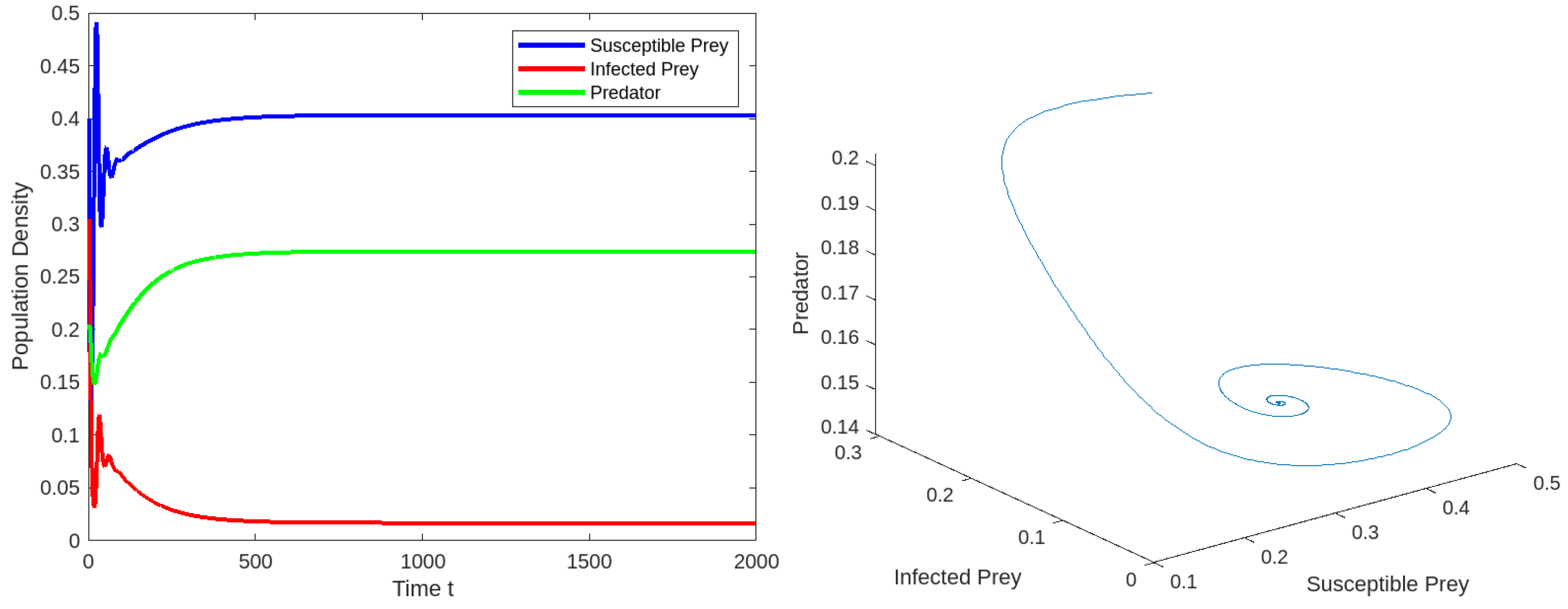
8. Numerical Simulations

In this section, we perform some numerical simulations on the system (2) in order to verify our theoretical findings. In this study, the susceptible prey-predator rate ($\omega$) and prey refuge ($\theta$) will be taken as important control parameters. Through the use of the MATLAB software, each of us performed various mathematical simulations where the particular parameter values are r = 0.5, $\beta$ = 0.2, d = 0.1, c = 0.5, $\gamma$ = 0.1, $h_2$ = 0.2, $\vartheta$ = 0.3, $\mu$ = 0.2, $\phi$ = 0.12, $h_1$ = 0.01, $\gamma$ = 0.1, $\omega$ = variable, $\theta$ = variable [8].

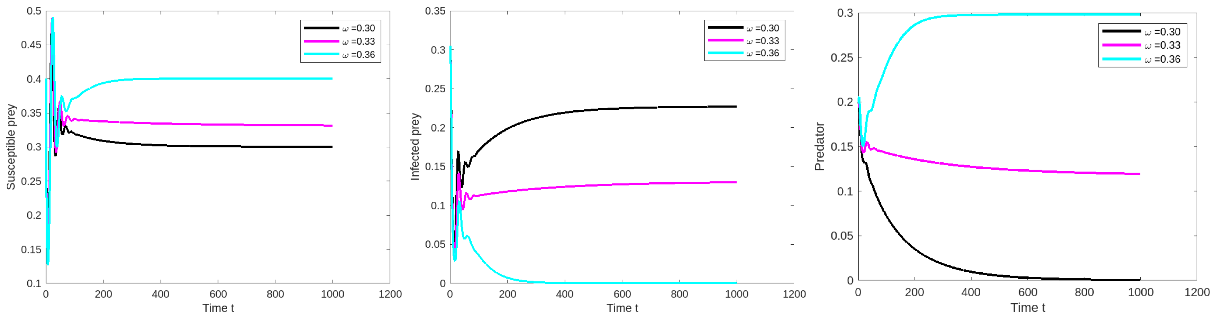
8.1. Effect of Varying the Susceptible Prey Predator Rate $\omega$

We should adjust the database variable

Table 2. The value of Parameter equation is (2).

Parameters	Numeric Value
r	0.5
$\beta$	0.2
d	0.1
c	0.5
$\gamma$	0.1
$h_2$	0.2
$\vartheta$	0.3
$\mu$	0.2
$\phi$	0.12
$h_1$	0.01
$\gamma$	0.1
$\omega$	variable
$\theta$	variable

as $\theta =0.2$. For the given limitation value, $E^{\ast }$ is stable at positive equilibrium point $\omega \ge 0.3$, as shown in Figure 1 and Figure 2.

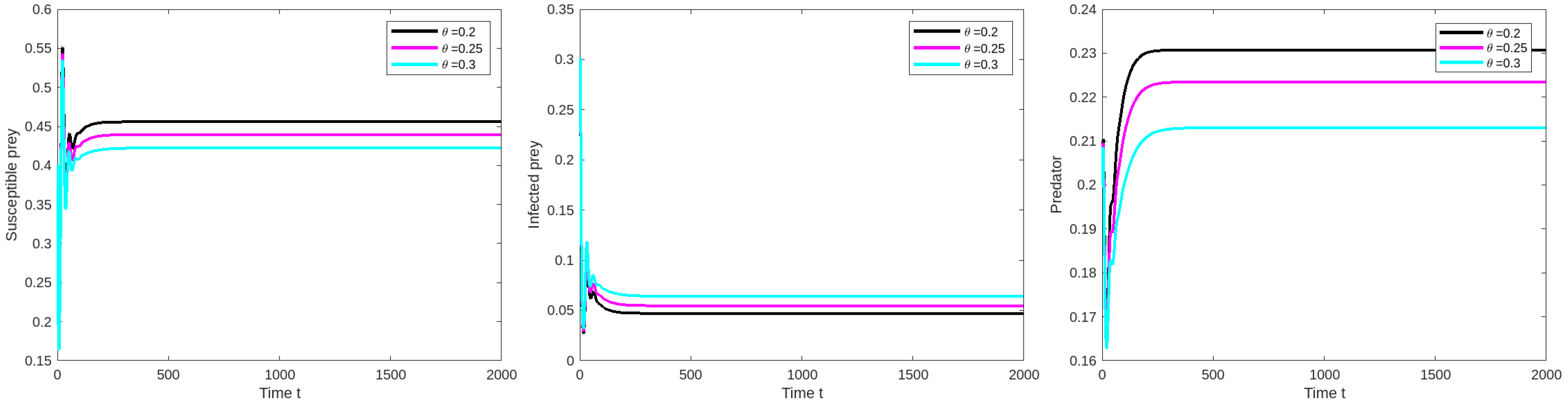
8.2. Effect of Varying the Prey Refuge $\theta$

We should adjust the database variable 2 as $\omega =0.3$. For the given limitation value, $E^{\ast }$ is stable at positive equilibrium point for $\theta \ge 0.2$, as shown in Figure 3.

9. Conclusions

In this study, we investigated the three-species food web eco-epidemiological model with prey refuge in an infected prey population and harvesting effect in both prey populations. Some mathematical results like positive invariance, positivity and boundedness were analysed in Equation (2). The local stability is assigned to each biologically feasible equilibrium point of the system. Global stability was analysed by a suitable Lyapunov function. Hopf bifurcation was analysed by bifurcation parameter $\left(\theta \right)$. Also, prey refuge $\left(\theta \right)$ and susceptible prey-predator rate $\left(\omega \right)$ was used as a control parameter. According to the analytical and numerical findings, the prey refuge and susceptible prey-predator rate has a major impact on the population. If we increase the susceptible prey predator rate and prey refuge in predator populations, the system loses its stability. This study shows the complex behavior of the proposed model.

References

1. Dimitrov, D.T.; Kojouharov, H.V. Complete mathematical analysis of predator–prey models with linear prey growth and Beddington–DeAngelis functional response. Appl. Math. Comput. 2005, 162, 523–538. [Google Scholar] [CrossRef]
2. Tripathi, J.P.; Abbas, S.; Thakur, M. A density dependent delayed predator–prey model with Beddington–DeAngelis type function response incorporating a prey refuge. Commun. Nonlinear Sci. Numer. Simul. 2015, 22, 427–450. [Google Scholar] [CrossRef]
3. Divya, A.; Sivabalan, M.; Ashwin, A.; Siva Pradeep, M. Dynamics of ratio dependent eco epidemiological model with prey refuge and prey harvesting. In Proceedings of the 1st International Online Conference on Mathematics and Applications, Online, 1–15 May 2023. [Google Scholar]
4. Cantrell, R.S.; Cosner, C. On the dynamics of predator–prey models with the Beddington–DeAngelis functional response. J. Math. Anal. Appl. 2001, 257, 206–222. [Google Scholar] [CrossRef]
5. Fan, M.; Kuang, Y. Dynamics of a nonautonomous predator–prey system with the Beddington–DeAngelis functional response. J. Math. Anal. Appl. 2004, 295, 15–39. [Google Scholar] [CrossRef]
6. Ashwin, A.; Sivabalan, M.; Divya, A.; Siva Pradeep, M. Dynamics of Holling type II eco-epidemiological model with fear effect, prey refuge, and prey harvesting. In Proceedings of the 1st International Online Conference on Mathematics and Applications, Online, 1–15 May 2023. [Google Scholar]
7. Melese, D.; Muhye, O.; Sahu, S.K. Dynamical behavior of an eco-epidemiological model incorporating prey refuge and prey harvesting. Appl. Appl. Math. Int. J. (AAM) 2020, 15, 28. [Google Scholar]
8. Tripathi, J.P.; Jana, D.; Tiwari, V. A Beddington–DeAngelis type one-predator two-prey competitive system with help. Nonlinear Dyn. 2018, 94, 553–573. [Google Scholar] [CrossRef]
Figure 1. At ω = 0.35 the time series and phase portrait of they system (2) at E .
Engproc 56 00306 g001
Figure 2. The compactness of susceptible prey, infected prey and predator population for the limitation values in Table 2 except θ = 0.2 and ω = 0.30 , 0.33 and 0.36 .
Engproc 56 00306 g002
Figure 3. The compactness of susceptible prey, infected prey and predator population for the limitation values in Table 2 except for ω = 0.3 and θ = 0.2 , 0.25 and 0.3 .
Engproc 56 00306 g003