Reconstructed Phase Spaces and LSTM Neural Network Ensemble Predictions ^†

Abstract

We present a novel approach that combines the concept of reconstructed phase spaces with neural network time-series predictions. The presented methodology aims to reduce the parametrization problem of neural networks and improve autoregressive neural network time-series predictions. First, the idea is to interpolate a dataset based on its reconstructed phase space properties and then filter an ensemble prediction based on its phase space properties. The corresponding ensemble predictions are made using randomly parameterized LSTM (Long Short-Term Memory) neural networks. These neural networks then produce a multitude of auto-regressive predictions, which are then filtered to achieve a smooth reconstructed phase space trajectory. Thus, we can circumvent the problem of parameterizing the neural network for each dataset individually. Here, the interpolation and the ensemble prediction aim to produce a smooth trajectory in a reconstructed phase space. The best results are compared to a single hidden layer LSTM neural network and benchmark results from the literature. The results show that the baseline predictions are outperformed for all three discussed datasets, and one of the benchmark results from the literature is bested by the presented approach.

1. Introduction

The rise of artificial intelligence, i.e., machine learning and deep learning, motivates many researchers to perform predictions and analyses based on historical data using these methods, rather than employing mechanistic expert models. The reason for making predictions in the first place is to answer important questions, e.g., future population estimates, predicting epileptic seizures, and estimating future stock market prices. The outcomes of these predictions are encouraging, e.g., solar radiation can be predicted using machine learning methods [1].

One reason for machine learning’s poor performance is an overall lack of data. A means of overcoming the lack of data for time-series analysis approaches is to employ an interpolation technique to increase the amount of data. Here, one can choose from many different techniques, such as polynomial, fractal [2], or stochastic interpolation methods [3]. In this article, we use an improved version of the Brownian multi-point bridges developed by [3], which is discussed and validated in detail in ref. [4]. For simplicity, we refer to this method as PhaSpaSto interpolation, which is an abbreviation for phase space trajectory smoothing stochastic interpolation.

Next, when it comes to the autoregressive prediction of time-series data, we want to consider the properties of the reconstructed phase space trajectories of a given set of time-series data, i.e., we want the reconstructed phase space trajectory of our prediction to be as smooth as possible.

Thus, we want to find out to what extent the idea of the reconstructed phase spaces of time-series data can be used to improve neural network time-series predictions. For this reason, we present the following scheme, depicted in Figure 1. We first interpolate a given time series using the discussed PhaSpaSto interpolation (Section 4); next, we employ the randomly parameterized neural networks developed in ref. [5] (Section 6), thus generating a multitude of different autoregressive predictions for each set of time-series data. Finally, we filter these predictions based on the smoothness of their reconstructed phase space trajectories, i.e., we want to keep only the smoothest phase space trajectories (Section 6.2).

This article is structured as follows. The current section, i.e., Section 1, provides a brief introduction and explains the developed scheme. Section 2 lists related work and briefly describes the connections to this article. Section 3 discusses the idea of reconstructed phase spaces and introduces the used terminology and notations. Next, Section 4 introduces the employed stochastic interpolation method, whereas Section 6 describes the employed neural network approach for autoregressive time-series prediction and the prediction filter. All datasets are described and plotted with their interpolation and corresponding phase space reconstructions in Section 5. Section 7 gives all prediction results. Section 8 concludes this article and gives ideas for future research.

2. Related Work

The presented research is mainly motivated by the findings of [2,4,5,6]. This section will briefly describe the mentioned publications, list them chronologically, i.e., by their publication date, and put them into context.

• Ref. [7]: This publication presents a method to determine if images are blurry. For this purpose, the second derivatives of grey-scale images are taken, and the corresponding variance over all pixels is analyzed. This concept is used in the presented article. We adapted the idea of variances of second derivatives, which is discussed in Section 4.2.
• Ref. [3]: This publication presents a novel stochastic interpolation technique where the idea of a Brownian bridge, i.e., a constrained fractional Brownian motion (fBm), is extended to more than two points, i.e., to multi-point fractional Brownian bridges. This method is the basis for the employed interpolation techniques and provides the population of random interpolations for the genetic algorithm.
• Ref. [2]: In this publication, a fractal interpolation to interpolate univariate time-series data is presented. This research suggests that different interpolation methods for univariate time-series data may yield predictions of different quality. Thus, as presented here, employing an attractor-based interpolation is an obvious next step compared to a fluctuation-based interpolation.
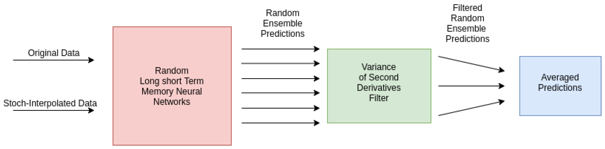
• Ref. [5]: This publication is a continuation of [2]. The fractal interpolation and LSTM neural network approach is continued as ensembles of predictions. Randomly parameterized LSTM neural networks are generated from non-, linear-, and fractal-interpolated data. Afterward, these predictions are filtered based on their signal complexities. Contrary to this publication, we test LSTM neural network predictions of stochastically interpolated data.
• Ref. [4]: This publication validates a stochastic interpolation based on the smoothness of reconstructed phase space trajectories and Brownian Bridges, i.e., the PhaSpaSto interpolation. The basic idea is to filter/improve a multitude of stochastic interpolations of the same time-series data using a genetic algorithm and the variance of second derivatives along a reconstructed phase space trajectory to generate smooth phase space embeddings.
  The interpolation technique developed in this paper is briefly described in Section 4 and used to improve the presented predictions.

3. Phase Space Reconstruction

First, we need to introduce the concept of reconstructed phase spaces [8,9].

We estimate a phase space embedding for all data under study. To find a suitable phase space embedding, one has to determine two parameters, the embedding dimension $d_E$ and the time delay $\tau$.

To estimate the time delay $\tau$, i.e., the delay between two consecutive time steps, we use the method based on the average information between two signals [10].

To estimate the embedding dimension $d_E$, we use the algorithm of false nearest neighbors [11].

The phase space embedding for a given signal $[x_1,x_2,\cdots ,x_n]$, thus, is

$$\overrightarrow{y}\left(i\right)=\left[x_i,x_{i+\tau },\cdots ,x_{i+(d_E-1)\ast \tau }\right],$$

(1)

and a corresponding three-dimensional phase space embedding, thus, is

$$\overrightarrow{y}\left(i\right)=\left[x_i,x_{i+\tau },x_{i+2\tau }\right].$$

(2)

4. PhaSpaSto Interpolation

The used interpolation technique consists of two parts: first, the multi-point fractional Brownian Bridges from [3], and second, a corresponding genetic algorithm choosing the best parts of the so-created fractional Brownian bridges.

4.1. Multi-Point Fractional Brownian Bridges

The employed genetic algorithm is fueled by a population of stochastically interpolated time-series data—in our case, multi-point fractional Brownian bridges. To generate these stochastically interpolated time-series data, multi-point fractional Brownian bridges [3] were used. Thus, we briefly summarize this approach.

We consider a Gaussian random process $X\left(t\right)$, whose covariance is defined as $C(t,t^{\prime })=\langle X\left(t\right)X\left(t^{\prime }\right)\rangle$. In the following, we focus on fractional Browian motion where the covariance is given according to $\langle X\left(t\right)X\left(t^{\prime }\right)\rangle =\frac{1}{2}\left(t^{2H}+t^{\prime 2H}-{|t-t^{\prime }|}^{2H}\right)$, where H is the Hurst exponent. To elucidate our interpolation scheme, we first define a so-called fractional Brownian bridge [12,13], which is a construction of fBm starting from 0 at $t=0$ and ending at $X_1$ at $t=t_1$, i.e.,

$$X^B\left(t\right)=X\left(t\right)-(X\left(t_1\right)-X_1)\frac{\langle X\left(t\right)X\left(t_1\right)\rangle }{\langle X{\left(t_1\right)}^2\rangle }.$$

(3)

This construction ensures that $X^B\left(t_1\right)=X_1$, which is also depicted in Figure 1. This single bridge can now be generalized to an arbitrary number of (non-equidistant) prescribed points $X_i$ at $t_i$ by virtue of a multi-point fractional Brownian bridge [3]

$$X^B\left(t\right)=X\left(t\right)-(X\left(t_i\right)-X_i){\sigma }_{ij}^{-1}〈X\left(t\right)X\left(t_j\right)〉,$$

(4)

where ${\sigma }_{ij}=\langle X\left(t_i\right)X\left(t_j\right)\rangle$ denotes the covariance matrix. Furthermore, we imply summation over identical indices. The latter linear operation on the Gaussian random process $X\left(t\right)$ ensures that the bridge takes on exactly the values $X_k$ at $t_k$, which can be seen from $X^B\left(t_k\right)=X\left(t_k\right)-(X\left(t_i\right)-X_i){\sigma }_{ij}^{-1}{\sigma }_{kj}=X\left(t_k\right)-(X\left(t_i\right)-X_i){\delta }_{ik}=X_k$, where ${\delta }_{ik}$ denotes the Kronecker delta. Hence, this method allows for the reconstruction of a sparse signal, where small-scale correlations are determined by the choice of the Hurst exponent H.

4.2. Genetic Algorithm

We build a simple genetic algorithm to find the best possible interpolation given the data’s phase space reconstruction using Taken’s theorem. We want our reconstructed phase space curve to be as smooth as possible and thus define the trajectory’s fitness as follows.

The basic idea is to use a concept from image processing, i.e., the blurriness of a picture, and apply it to phase space trajectories. We want our trajectory to be as blurry, i.e., as smooth, as possible. In image processing, the blurriness is determined via second-order derivatives of grey-scale images at each pixel [7]. We employ this concept, but instead of using it at each pixel, we calculate the variance of second-order derivatives along our phase space trajectories. Similar to the idea from image processing, where the low variance of second-order derivatives implies more blurriness, curves with a low variance of second-order derivatives exhibit comparatively smooth trajectories. The reason here is intuitively apparent: whereas curves with a high variance of second-order derivatives have a range of straight and pointy sections, curves with a low variance of second-order derivatives have a similar curvature along the trajectory and thus are smoother. Hence, in order to guarantee smoothness along the trajectory, we want this variance to be as low as possible, which thus is our loss L. Concluding, our fitness is maximal when our loss L is minimal.

Again, we start with the phase space vector and the corresponding embedding dimension $d_E$ and time delay $\tau$ (see Section 3) of each signal as

$$\overrightarrow{y}\left(i\right)=\left[x_i,x_{i+\tau },\cdots ,x_{i+(d_E-1)·\tau }\right].$$

(5)

Thus, we have one component for each dimension of the phase space. Consequently, we can write the individual components as

$$y_j\left(i\right)=x_{i+\left(j-1\right)\ast \tau },$$

(6)

where $j=1,2,\cdots ,d_E$. We then take the second-order finite difference central derivative of a discrete function [14]

$$u_j^{″}\left(i\right)=x_{i+\left(j-1\right)\ast \tau +1}-2x_{i+\left(j-1\right)\ast \tau }+x_{i+\left(j-1\right)\ast \tau -1},$$

(7)

at each point, and for each component. Next, we add up all the components as

$$u^{″}\left(i\right)=\sqrt{{\sum }_{j=1}^{d_E}{u}_j^{″}{\left(i\right)}^2}.$$

(8)

Then, finally, we use the variance of the absolute values of second derivatives along the phase space curve as our loss L of a phase space trajectory:

$$L={\mathrm{Var}}_i\left[u^{″}\left(i\right)\right].$$

(9)

The employed genetic algorithm consists of the following building blocks.

A candidate solution is an interpolated time series using a random Hurst exponent $H\in \left(0;1\right)$. The corresponding population of candidates is, e.g., 1000 of these stochastically interpolated time-series data with random Hurst exponents. A population of interpolated time-series data is generated using the multi-point Brownian bridges such that, for each member of the population, a random Hurst exponent with $H\in \left(0;1\right)$ is chosen, which then defines the interpolation of the member of the population. After generating the population, all members are sorted with respect to their fitness, i.e., the lower the loss L, the better an interpolation is. The mating is implemented such that only the best 50%, with respect to fitness, can mate to produce new offspring. The mating is done such that, for every gene, i.e., each interpolation between two data points, there is a 50:50 chance to inherit it from either one of the parents. The mutation was implemented such that, in each generation, there is a 20% chance that a randomly chosen interpolated time series is replaced with a new interpolated time series within a corresponding randomly chosen new Hurst exponent. Moreover, we implemented a criterion for aborting the program, which was fulfilled if the population fitness mean did not change for ten generations. This described procedure was then performed for 1000 generations. However, the 1000 generations were never reached, as the criterion for abortion was always triggered, and the program was ended, thus yielding the best interpolation with respect to the fitness of the phase space trajectories before reaching the 1000th generation.

5. Datasets

We chose three datasets to test and demonstrate our approach. Two of the featured datasets are from the Time Series Data Library [15] and thus are known test datasets and provide us with benchmark results, which are discussed in Section 7.4.

The third dataset is the annual maize yields in Austria, which can be obtained from http://www.fao.org/faostat/, accessed on 21 July 2022. This third dataset is considered the most challenging of the three datasets for two reasons. First, it is an agricultural dataset, i.e., it is affected by the weather, genetic improvements of the plants, varying fertilization strategies, etc., meaning that we will most likely not discover any reasonable seasonalities and or trends, despite the apparent increase in maize yields due to various improvements in agriculture. Second, this dataset is collected annually for all of Austria, i.e., a lot of the information contained in the dataset is lost due to the annual and regional averaging. Thus, we conclude that it will be challenging or impossible to predict annual maize yields several years ahead effectively.

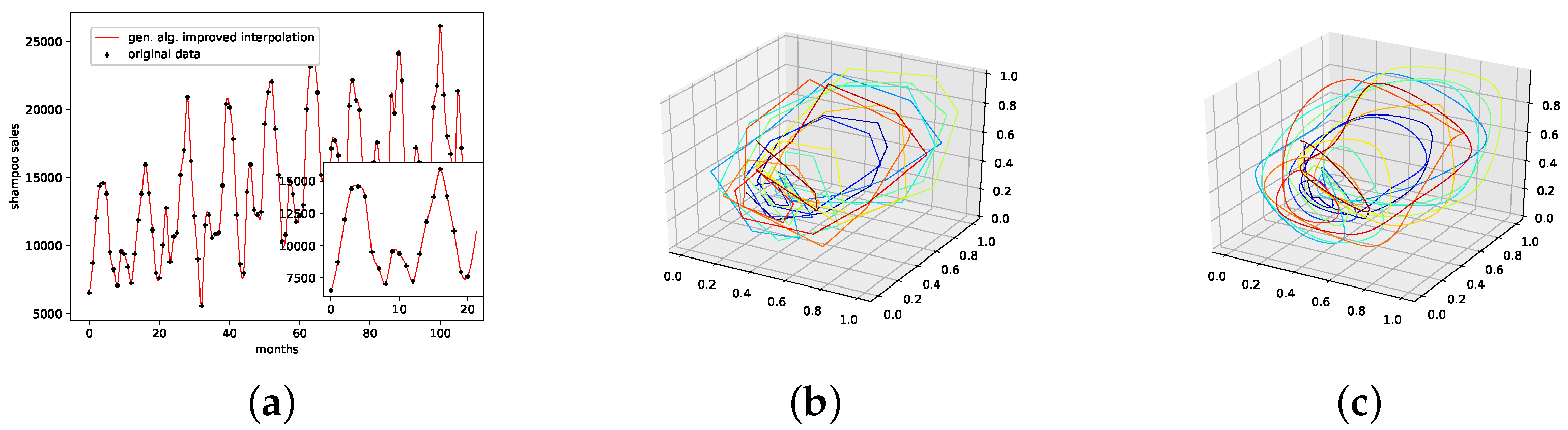
5.1. Car Sales in Quebec Dataset

This is a dataset from the Time Series Data Library [15]. It depicts monthly car sales in Quebec from January 1960 to December 1968, with an overall 108 data points.

The corresponding phase space embedding, with a time delay $\tau =1$, was detrended by subtracting a linear fit from the data and normalized such that the range of all data is between $\left[0,1\right]$. The interpolated time series and the corresponding reconstructed phase space are depicted in Figure 2.

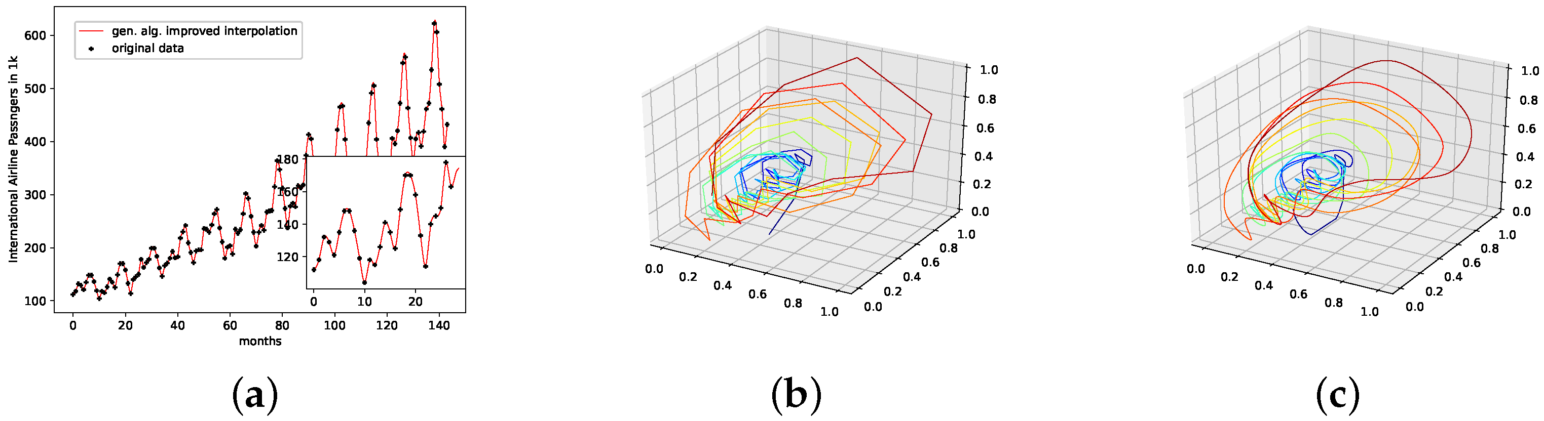
5.2. Monthly International Airline Passengers Dataset

This is a dataset from the Time Series Data Library [15]. It depicts monthly international airline passengers from January 1949 to December 1960, with an overall 144 data points, given in units of 1000.

The corresponding phase space embedding, with a time delay $\tau =1$, was detrended by subtracting a linear fit from the data and normalized such that the range of all data is between $\left[0,1\right]$. The interpolated time series and the corresponding reconstructed phase space are depicted in Figure 3.

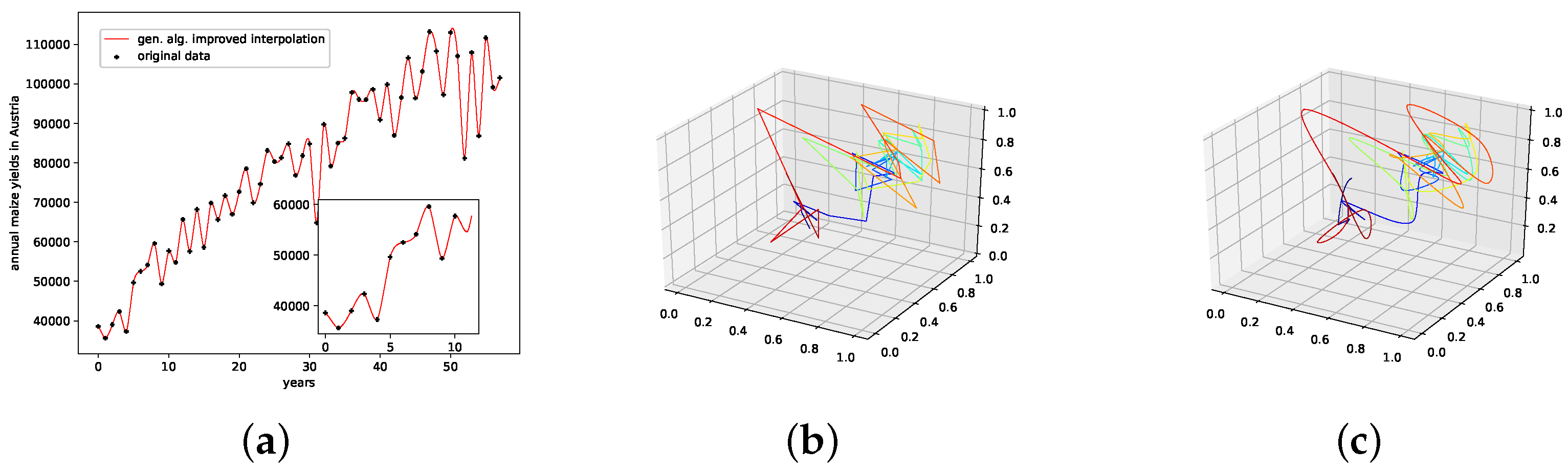
5.3. Annual Maize Yields in Austria

This is a dataset of the annual yields of maize in Austria ranging from 1961 to 2017, with an overall 57 data points. This dataset can be downloaded at http://www.fao.org/faostat/, accessed on 21 July 2022. The corresponding phase space embedding, with a time delay $\tau =1$ and an embedding dimension of $d_E=3$, was detrended by subtracting a linear fit from the data and normalized such that the range of all data is between $\left[0,1\right]$. The interpolated time series and the corresponding reconstructed phase space are depicted in Figure 4.

5.4. Data Preprocessing

Two steps of preprocessing were performed before forecasting the featured datasets. First, each dataset was made stationary by subtracting a linear fit. Second, each dataset was scaled to $\left[0.1,0.9\right]$.

Finally, each dataset was split into a train and test dataset with an $80\%/20\%$ ratio.

6. LSTM Neural Network Time-Series Prediction

LSTMs are a category of recurrent neural networks (RNNs). RNNs are capable of using feedback or recurrent connections to cope with time-series data.

LSTMs [16] feature a component called a memory block to enhance their capability to model long-term dependencies. This memory block is a recurrently connected subnet containing two functional modules, i.e., the memory cell and the corresponding gates. The task of the memory cell is to remember the temporal state of the neural network. On the other hand, the gates are responsible for controlling the information flow and consist of multiplicative units.

6.1. Randomly Parameterized Neural Networks

In this article, we are using an approach developed in [5]. The idea is to generate many randomly parameterized neural networks to build ensemble predictions based on the phase space properties of the autoregressively produced predictions. An autoregressive prediction is a one-step-at-a-time prediction, whereas old outputs are used as inputs for the next step.

These randomly parameterized neural networks feature one to five hidden LSTM layers, a hard sigmoid activation function in the hidden and input layers, and a rectified linear unit as the output activation function. No dropout criterion or regularization was used.

We used the following ranges for the parameters for our randomly parameterized neural network implementation.

• Number of input nodes: 1 → size of the training data − 1
• Number of neurons for each hidden layer: 1 → 50
• Batchsizes: 2 → 128
• Epochs: 1 → 50

We used LSTM architectures for this research, one can use any type of neural network cell for this approach.

6.2. Prediction Filter

The so-generated autoregressive predictions are then filtered using the criterion for smooth phase space trajectories from Section 4.2, i.e., we want the variance of second derivatives along a reconstructed phase space trajectory to be as low as possible. We thus randomly chose 1 to 10 predictions from the whole set of predictions. Next, these predictions are averaged to form an ensemble prediction. This ensemble prediction is merged with the training data. Then, the variance of second derivatives along the phase space trajectory is analyzed. This process is repeated 1 million times. The set of averaged predictions with the lowest variance of second derivatives is kept. On all plots, this procedure is referred to as loss_rand.

7. Experiments and Results

In this Section, we provide the experimental setup and the corresponding results.

First, each dataset was interpolated using PhaSpaSto interpolation (Section 4) with varying interpolation points. For the monthly international airline passengers and the car sales in Quebec datasets, interpolations with the following numbers of interpolation points were performed: $N_I=\{1,3,5,7,9,11,13\}$. For the annual maize yields in Austria, this range was changed to $N_I=\{9,11,13,15\}$ to save computational resources. Further, we produced 500 randomly parameterized neural network predictions for the monthly international airline passengers and car sales in Quebec datasets. In contrast, for the annual maize yields in Austria dataset, 1000 of these predictions were produced. These multitudes of predictions were created for the non-interpolated and the interpolated datasets. As initially mentioned, the whole scheme is depicted in Figure 1.

All of these predictions were analyzed using the root mean squared error (RMSE). Here, we used the RMSE on both a normalized dataset, i.e., the dataset and the prediction are scaled to be $\in \left[0,1\right]$ (denoted as RMSE [0, 1], Equation (10)), and the regular dataset and prediction (denoted as RMSE, Equation (10)).

All errors for all datasets are collected in

Table 1. Results for all datasets and experiments, i.e., interpolated, non-interpolated, filtered, and unfiltered.

Data	Approach	RMSE [0, 1]	RMSE
Car Sales in Quebec	not interpolated, unfiltered	0.31148	6395.04838
Car Sales in Quebec	not interpolated, filtered	0.11635	1927.52494
Car Sales in Quebec	stoch. interpolated, $N_I=13$, unfiltered	0.24762	5104.42560
Car Sales in Quebec	stoch. interpolated, $N_I=1$, filtered	0.07958	1617.40461
Monthly International Airline Passengers	not interpolated, unfiltered	0.19676	101.92294
Monthly International Airline Passengers	not interpolated, filtered	0.06823	35.34095
Monthly International Airline Passengers	stoch. interpolated, $N_I=13$, unfiltered	0.17180	86.28560
Monthly International Airline Passengers	stoch. interpolated, $N_I=9$, filtered	0.05286	21.20474
Annual Maize Yields Austria	not interpolated, unfiltered	0.23536	18,253.10327
Annual Maize Yields Austria	not interpolated, filtered	0.16424	12,737.42487
Annual Maize Yields Austria	stoch. interpolated, $N_I=15$, unfiltered	0.20499	15,442.32505
Annual Maize Yields Austria	stoch. interpolated, $N_I=15$, filtered	0.14563	11,227.39159

. The corresponding plots for the car sales in Quebec dataset are collected in Figure 5, the results for the monthly international airline passengers are plotted in Figure 6, and finally, the results for the annual maize yields in Austria are depicted in Figure 7. Further, we discuss each dataset separately in the following.

$$RMSE={\left(\frac{1}{n}\sum _{i=1}^n{\left[{\widehat{x}}_i-x_i\right]}^2\right)}^{\frac{1}{2}},$$

(10)

Here, ${\widehat{x}}_i$ are the predicted values, $x_i$ is the ground truth, and n is the number of samples.

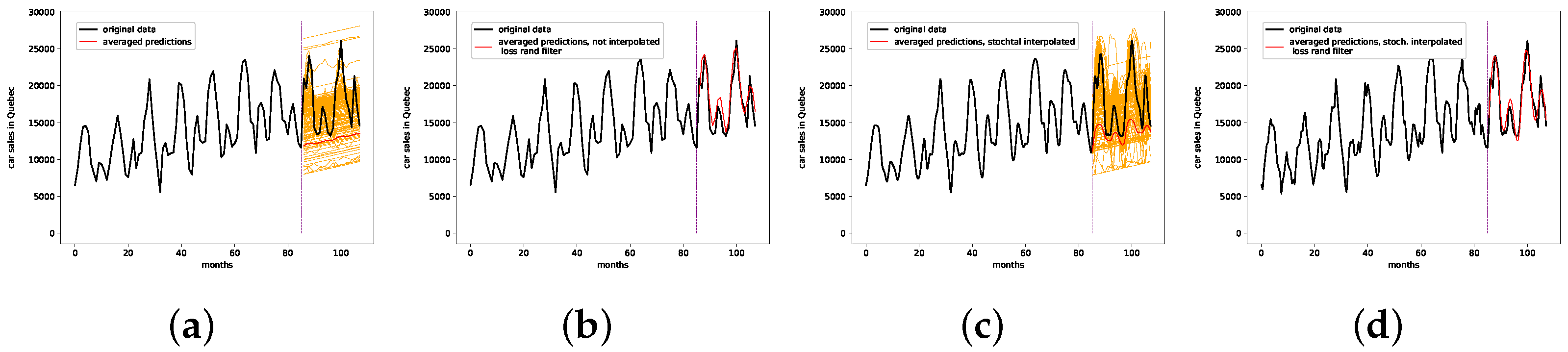
7.1. Car Sales in Quebec Dataset

All errors for the car sales in Quebec dataset are collected in Table 1, and the corresponding plots are collected in Figure 5.

When comparing the errors for the results with and without interpolation, we see that the interpolated results are reduced, i.e., the unfiltered, interpolated results have a lower error than the unfiltered, not interpolated ones. The same is true for the filtered results.

Next, the filtered results consistently drastically outperformed the unfiltered ones. Exactly this behavior is depicted in Figure 5. The overall best result is the interpolated and filtered prediction approach, which can be seen in Figure 5d.

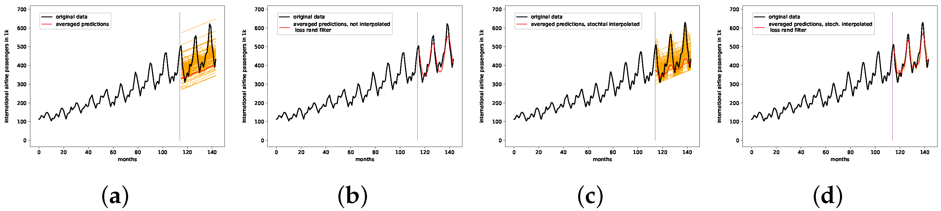
7.2. Monthly International Airline Passengers

All errors for the monthly international airline passengers dataset are collected in Table 1, and the corresponding plots are collected in Figure 6.

When comparing the errors for the results with and without interpolation, we see that the errors for the interpolated results are reduced, i.e., the unfiltered interpolated results have a lower error than the unfiltered, not interpolated ones. The same is true for the filtered results.

Next, the filtered results always drastically outperformed the unfiltered ones. Exactly this behavior is depicted in Figure 6. The overall best result is the interpolated and filtered prediction approach, which can be seen in Figure 6d.

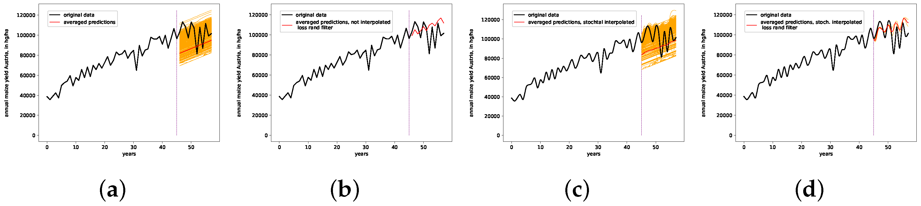
7.3. Annual Maize Yields in Austria Dataset

All errors for the monthly international airline passengers dataset are collected in Table 1, and the corresponding plots are collected in Figure 7.

When comparing the errors for the results with and without interpolation, we see that the interpolated results are reduced, i.e., the unfiltered, interpolated results have a lower error than the unfiltered, not interpolated ones. The same is true for the filtered results.

Next, the filtered results consistently drastically outperformed the unfiltered ones. Exactly this behavior is depicted in Figure 7. The overall best result is the interpolated and filtered prediction approach, which can be seen in Figure 7d.

This dataset is considered to be the most difficult of the three featured datasets, and although our predictions are still off, as can be seen in Figure 7d, the performed procedures, i.e., PhaSpaSto interpolation and the prediction filter, do improve the accuracy of the forecast. Further, the result depicted in Figure 7d suggests that the employed neural networks learned some inherent behavior, especially when taking into account the initial variations after the train/test cut.

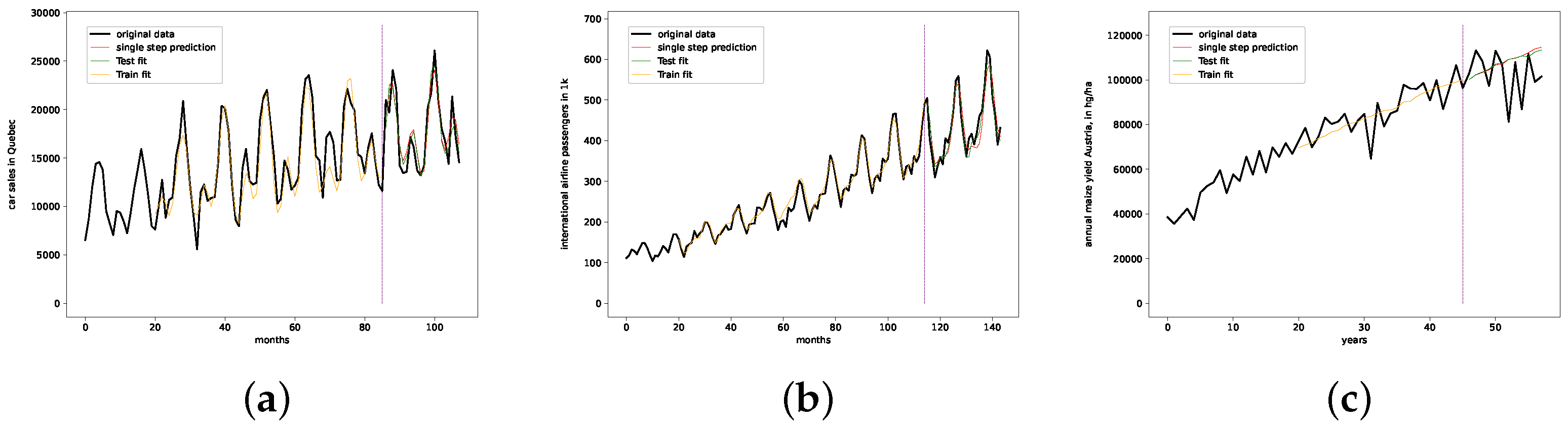
7.4. Benchmark and Baseline Predictions

We finally provide some baseline and benchmark results for the conducted experiments. We used an LSTM neural network with one hidden layer as a baseline prediction. Each neural network was trained with a batch size of 2 and varying epochs. Further, verbose was set to 2. For the activation of the neural network, hard_sigmoid was chosen, and the activation function of the output layer was relu. For the initialization, glorot_uniform was used for the LSTM layer, orthogonal was used as the recurrent initializer, and glorot_uniform for the Dense layer. For the LSTM layer, the bias was set to use_bias=True, with a corresponding bias_initializer="zeros". Further, no constraints, regularizers, or dropout criteria were used for the recurrent and the Dense layers. As an optimizer, rmsprop was used and the loss was calculated using mean_squared_error. The output node returned only one result, i.e., the next time step. The varying architectures are collected in

Table 2. Errors for the baseline predictions for each dataset.

Data	Architecture	RMSE [0, 1]	RMSE
Car Sales in Quebec	20 input nodes 30 hidden layer neurons 45 training epochs	0.08593	1764.38996
Monthly International Airline Passengers	20 input nodes 30 hidden layer neurons 40 training epochs	0.05899	30.56100
Annual Maize Yields Austria	20 input nodes 30 hidden layer neurons 18 training epochs	0.16617	12,886.99962

and the corresponding predictions are depicted in Figure 8.

The featured baseline predictions, though reasonable, are consistently outperformed by the interpolated filtered results from our main experiments—see Table 1—in terms of RMSE. Here, we want to highlight that the baseline neural network did not capture the characteristics of the annual maize yields dataset. This may be due to poor parameterization or the fact that a single hidden layer is not sufficient to capture the dynamics of this dataset. Still, we tuned the employed neural networks by hand, and the results for the other dataset show that neural networks of these sizes are sufficient for univariate time-series data of this length. The best ensemble result, in comparison, provides a drastically improved result compared to the baseline prediction.

When it comes to benchmark results from the literature, we found the best result for the monthly international airline passengers dataset in ref. [17], with an RMSE of $13.0$ for a hybrid MLP-ARIMA approach, which is superior to our baseline of $30.6$ and our best ensemble result of $21.2$. Thus, we conclude that our ensemble approach with the presented specifications cannot outperform state-of-the-art methods for this dataset.

For the monthly car sales in Quebec dataset, we found a comparable result in ref. [18], with an RMSE $\left[0,1\right]$ of $0.08143$ for the additive Holt–Winters method. Our baseline LSTM result for this dataset has an RMSE $\left[0,1\right]$ of $0.08593$ and our best ensemble results is at $0.07958$. We conclude that our ensemble prediction is able to outperform the best results from ref. [18] for this dataset.

As far as the authors know, there is no benchmark result for the annual maize yields in Austria dataset. Thus, we stick to the previously presented baseline prediction, which is outperformed by the presented ensemble prediction.

7.5. Summary

We briefly summarize our findings and point out the main results below.

(1)

The presented stochastic interpolation method—for simplicity, referred to as PhaSpaSto interpolation—can be used to improve retrogressive neural network time-series predictions. This is supported by the findings of Table 1. Here, we can see that both the filtered and unfiltered interpolated results outperformed those without interpolation. The same is true for all filtered results, i.e., the interpolated results always outperformed the unfiltered ones. These results are depicted in Figure 5, Figure 6 and Figure 7.

(2)

Filtering the multitude of predictions based on the second derivatives along their reconstructed phase space portraits drastically improved the results for all datasets. The corresponding results are, again, collected in Table 1 and Figure 5, Figure 6 and Figure 7.

(3)

The presented interpolated and filtered approach outperformed the baseline and benchmark predictions for the monthly car sales in Quebec dataset, discussed in Section 7.4.

Though the interpolated and filtered ensemble approach did outperform a given baseline prediction for the monthly international airline passengers dataset, the featured benchmark prediction from the literature still outperformed our approach on this dataset.

We provide a baseline prediction for the annual maize yields in Austria dataset, which was outperformed using our interpolated and filtered ensemble approach, discussed in Section 7.4. We cannot provide a benchmark result from the literature for this dataset.

(4)

The employed neural network ensembles were not individually parameterized for each dataset. Instead, we filtered the predictions according to the phase space properties of each dataset. Thus, we could circumvent the problem of parameterizing neural networks.

8. Conclusions

This article presents an experiment to test the applicability of a novel interpolation method—for simplicity, abbreviated as PhaSpaSto interpolation—combined with randomly parameterized neural network autoregressive predictions. These predictions are then filtered using the variance of second derivatives along a reconstructed phase space trajectory to only keep forecasts that ensure a smooth phase space trajectory.

First, a given time series is interpolated using the featured interpolation method. It is forecast by generating multiple differently parameterized neural networks, each providing an autoregressive prediction of the data under study. Finally, this multitude of predictions is filtered such that the result guarantees a smooth reconstructed phase space trajectory.

The results show that this novel approach outperforms the provided baseline predictions. Further, we were able to best a given benchmark result from the literature for one of the three discussed datasets.

The concept of reconstructed phase spaces can be applied to interpolate time series to guarantee a smooth phase space trajectory, which, in turn, improves the accuracy of our neural network predictions. Further, filtering ensemble predictions based on their phase space properties, i.e., the smoothness of their phase space trajectories, improves the presented ensemble predictions. Moreover, we can circumvent the problem of parameterizing neural networks by generating many predictions and filtering them based on their phase space properties.

Ideas for future research in this field are, e.g., to test the presented filter on other state-of-the-art ensemble approaches or to test the robustness of neural network predictions using the presented PhaSpaSto and related interpolation techniques. We further want to highlight that the proposed methodology improves the accuracy on the featured annual maize yields dataset, which the authors expected to be a challenging dataset. Thus, another idea for future research might be to specifically target challenging time-series prediction problems, such as forecasting agricultural or financial time-series data.

References

1. Voyant, C.; Notton, G.; Kalogirou, S.; Nivet, M.L.; Paoli, C.; Motte, F.; Fouilloy, A. Machine learning methods for solar radiation forecasting: A review. Renew. Energy 2017, 105, 569–582. [Google Scholar] [CrossRef]
2. Raubitzek, S.; Neubauer, T. A fractal interpolation approach to improve neural network predictions for difficult time series data. Expert Syst. Appl. 2021, 169, 114474. [Google Scholar] [CrossRef]
3. Friedrich, J.; Gallon, S.; Pumir, A.; Grauer, R. Stochastic Interpolation of Sparsely Sampled Time Series via Multipoint Fractional Brownian Bridges. Phys. Rev. Lett. 2020, 125, 170602. [Google Scholar] [CrossRef] [PubMed]
4. Raubitzek, S.; Neubauer, T.; Friedrich, J.; Rauber, A. Interpolating Strange Attractors via Fractional Brownian Bridges. Entropy 2022, 24, 718. [Google Scholar] [CrossRef] [PubMed]
5. Raubitzek, S.; Neubauer, T. Taming the Chaos in Neural Network Time Series Predictions. Entropy 2021, 23, 1424. [Google Scholar] [CrossRef] [PubMed]
6. Raubitzek, S.; Neubauer, T. Combining Measures of Signal Complexity and Machine Learning for Time Series Analyis: A Review. Entropy 2021, 23, 1672. [Google Scholar] [CrossRef] [PubMed]
7. Pech-Pacheco, J.; Cristobal, G.; Chamorro-Martinez, J.; Fernandez-Valdivia, J. Diatom autofocusing in brightfield microscopy: A comparative study. In Proceedings of the 15th International Conference on Pattern Recognition, ICPR-2000, Barcelona, Spain, 3–7 September 2000; Volume 3, pp. 314–317. [Google Scholar] [CrossRef]
8. Takens, F. Detecting strange attractors in turbulence. In Dynamical Systems and Turbulence, Warwick 1980, Lecture Notes in Mathematics; Rand, D., Young, L.S., Eds.; Springer: Berlin/Heidelberg, Germany, 1981; Volume 898, pp. 366–381. [Google Scholar]
9. Packard, N.H.; Crutchfield, J.P.; Farmer, J.D.; Shaw, R.S. Geometry from a Time Series. Phys. Rev. Lett. 1980, 45, 712–716. [Google Scholar] [CrossRef]
10. Fraser, A.M.; Swinney, H.L. Independent coordinates for strange attractors from mutual information. Phys. Rev. A 1986, 33, 1134–1140. [Google Scholar] [CrossRef] [PubMed]
11. Rhodes, C.; Morari, M. The false nearest neighbors algorithm: An overview. Comput. Chem. Eng. 1997, 21, S1149–S1154. [Google Scholar] [CrossRef]
12. Delorme, M.; Wiese, K.J. Extreme-value statistics of fractional Brownian motion bridges. Phys. Rev. E 2016, 94, 052105. [Google Scholar] [CrossRef] [PubMed] [Green Version]
13. Sottinen, T.; Yazigi, A. Generalized Gaussian bridges. Stoch. Process. Appl. 2014, 124, 3084–3105. [Google Scholar] [CrossRef] [Green Version]
14. Quarteroni, A.; Sacco, R.; Saleri, F. Numerical Mathematics, 2nd ed.; Springer: Berlin/Heidelberg, Germany, 2007; Volume 37. [Google Scholar] [CrossRef] [Green Version]
15. Hyndman, R.; Yang, Y. Time Series Data Library v0.1.0. 2018. Available online: pkg.yangzhuoranyang.com/tsdl (accessed on 1 July 2022).
16. Hochreiter, S.; Schmidhuber, J. Long Short-term Memory. Neural Comput. 1997, 9, 1735–1780. [Google Scholar] [CrossRef]
17. Domingos, S.d.O.; de Oliveira, J.F.; de Mattos Neto, P.S. An intelligent hybridization of ARIMA with machine learning models for time series forecasting. Knowl.-Based Syst. 2019, 175, 72–86. [Google Scholar]
18. Shah, V. A Comparative Study of Univariate Time-Series Methods for Sales Forecasting. Master’s Thesis, University of Waterloo, Waterloo, ON, Canada, 2020. [Google Scholar]
Figure 1. Schematic depiction of the filtering process. The whole pipeline is applied, first, to the original non-interpolated data, and second, to the stoch.-interpolated data set.
Engproc 18 00040 g001
Figure 2. Time-series and attractor plots for the annual car sales in Quebec dataset. (a) Stoch. interpolated, 13 interpolation points, time-series plot; (b) non-interpolated, reconstructed attractor plot, detrended, normalized; (c) stoch.-interpolated, 13 interpolation points, reconstructed attractor plot, detrended, normalized. The rainbow colors in the phase space plots correspond to different steps in time. The spectrum starts with blue (early) and ends with red (later).
Engproc 18 00040 g002
Figure 3. Time-series and attractor plots for the monthly international airline passengers dataset. (a) Stoch.-interpolated, 13 interpolation points, time-series plot; (b) non-interpolated, reconstructed attractor plot, detrended, normalized; (c) stoch.-interpolated, 13 interpolation points, reconstructed attractor plot, detrended, normalized. The rainbow colors in the phase space plots correspond to different steps in time. The spectrum starts with blue (early) and ends with red (later).
Engproc 18 00040 g003
Figure 4. Time-series and attractor plots for the annual maize yields in Austria data set. (a) Stoch.-interpolated, 13 interpolation points, time-series plot; (b) non -interpolated, reconstructed attractor plot, detrended, normalized; (c) stoch.-interpolated, 13 interpolation points, reconstructed attractor plot, detrended, normalized. The rainbow colors in the phase space plots correspond to different steps in time. The spectrum starts with blue (early) and ends with red (later).
Engproc 18 00040 g004
Figure 5. Autoregressive prediction results for the car sales in Quebec dataset. (a) Non-interpolated, non-filtered; (b) non-interpolated, filtered; (c) stoch. interpolated, 13 interpolation points, non-filtered; (d) stoch. interpolated, 1 interpolation point, filtered.
Engproc 18 00040 g005
Figure 6. Autoregressive prediction results for the car sales in Quebec dataset. (a) Non-interpolated, non-filtered; (b) non-interpolated, filtered; (c) stoch. interpolated, 13 interpolation points, non-filtered; (d) stoch. interpolated, 9 interpolation points, filtered.
Engproc 18 00040 g006
Figure 7. Autoregressive prediction results for the car sales in Quebec dataset. (a) Non-interpolated, non-filtered; (b) non-interpolated, filtered; (c) stoch. interpolated, 15 interpolation points, non-filtered; (d) stoch. interpolated, 15 interpolation points, filtered.
Engproc 18 00040 g007
Figure 8. LSTM baseline predictions. The red line denotes the autorgressive single step-by-step prediction, which is featured in Table 2. (a) Car sales in Quebec dataset; (b) monthly international airline passengers dataset; (c) annual maize yields in Austria dataset.
Engproc 18 00040 g008