Proceeding Paper

The Bootstrap for Testing the Equality of Two Multivariate Stochastic Processes with an Application to Financial Markets †

by
Ángel López-Oriona
1,* and
José A. Vilar
1,2
1
Research Group MODES, Research Center for Information and Communication Technologies (CITIC), University of A Coruña, 15071 A Coruña, Spain
2
Technological Institute for Industrial Mathematics (ITMATI), 15705 Santiago de Compostela, Spain
*
Author to whom correspondence should be addressed.
Presented at the 8th International Conference on Time Series and Forecasting, Gran Canaria, Spain, 27–30 June 2022.
Eng. Proc. 2022, 18(1), 38; https://doi.org/10.3390/engproc2022018038
Published: 8 July 2022
(This article belongs to the Proceedings of The 8th International Conference on Time Series and Forecasting)

Abstract

:
The problem of testing the equality of generating processes of two multivariate time series is addressed in this work. To this end, we construct two tests based on a distance measure between stochastic processes. The metric is defined in terms of the quantile cross-spectral densities of both processes. A proper estimate of this dissimilarity is the cornerstone of the proposed tests. Both techniques are based on the bootstrap. Specifically, extensions of the moving block bootstrap and the stationary bootstrap are used for their construction. The approaches are assessed in a broad range of scenarios under the null and the alternative hypotheses. The results from the analyses show that the procedure based on the stationary bootstrap exhibits the best overall performance in terms of both size and power. The proposed techniques are used to answer the question regarding whether or not the dotcom bubble crash of the 2000s permanently impacted global market behavior.

1. Introduction

Comparison of time series often arises in multiple fields including machine learning, finance, economics, computer science, biology, medicine, physics, and psychology, among many others. For instance, it is not uncommon for an investor to have to determine if two particular assets show the same dynamic behavior over time based on historical data. In the same way, a physician often needs to find out to what extent two ECG signals recorded from different subjects exhibit similar patterns. There exist a wide variety of tools that have been used for these and similar purposes, including cluster analysis [1], classification [2], outlier detection [3], and comparisons through hypotheses tests [4]. It is worth highlighting that these techniques have mainly focused on univariate time series (UTS) [5], while the study of multivariate time series (MTS) has been given limited consideration [6].
In the context of hypotheses tests for time series, spectral quantities have played an important role. Specifically, testing for the equality of spectral densities has found substantial interest in the literature. Ref. [7] proposed a test for comparing spectral densities of stationary time series with unequal sample sizes. The procedure generalizes the class of tests presented in [8], which are based on an estimate of the L 2 -distance between the spectral density and its best approximation under the null hypothesis. Ref. [9] constructed a non-parametric test for the equality of spectral density matrices based on an L 2 -type statistic.
This work is devoted to constructing procedures to test for the equality of the so-called quantile cross-spectral density (QCD) between two independent MTS. Specifically, let X t ( 1 ) and X t ( 2 ) be two independent, d-variate, real-valued, strictly stationary stochastic processes. We fix a frequency ω [ π , π ] and a pair of probability levels, τ , τ [ 0 , 1 ] , and we denote the corresponding QCD matrices by f ( i ) ( ω , τ , τ ) , i = 1 , 2 . The hypotheses we consider can be stated as
H 0 : f X t ( 1 ) = f X t ( 2 ) against H 1 : f X t ( 1 ) f X t ( 2 ) ,
where f X t ( 1 ) and f X t ( 2 ) are the corresponding sets of QCD matrices defined as
f X t ( i ) = { f ( i ) ( ω , τ , τ ) , ω [ π , π ] , τ , τ [ 0 , 1 ] } .
where i = 1 , 2 . In order to perform the test in (1), we rely on a distance measure between stationary stochastic processes, so-called d Q C D , which has already being utilized in several MTS data mining tasks [6,10,11,12]. This metric is simply the Euclidean distance between two complex vectors constructed by concatenating the terms in each collection of matrices (2) for some finite set of frequencies and probability levels. Hence, an equivalence occurs between the null hypothesis in (1) and the distance d Q C D being zero for every possible set, making an estimate of this metric an appropriate tool to carry out the test in (1). The high ability of d Q C D to detect every possible discrepancy between stochastic processes was shown in our previous work [10].
Two methods to perform the test in (1) are introduced in this manuscript. They are based on the moving block bootstrap (MBB) (see [13,14]) and the stationary bootstrap (SB) (see [15]). Both approaches are compared in terms of size and power by means of a broad simulation study. Finally, the tests are applied to answer the question regarding whether or not the dotcom bubble burst of 2000 changed the global behavior of financial markets.
The rest of the paper is organized as follows. The distance d Q C D between stochastic processes is defined in Section 2. The two techniques to carry out the test in (1) are presented in Section 3. The results from the simulation study performed to compare the proposed tests are reported in Section 4. Section 5 contains the financial application and Section 6 concludes.

2. A Distance Measure between Stochastic Processes

Let { X t , t Z } = { ( X t , 1 , , X t , d ) , t Z } be a d-variate real-valued strictly stationary stochastic process. Denote by F j the marginal distribution function of X t , j , j = 1 , , d , and by q j ( τ ) = F j 1 ( τ ) , τ [ 0 , 1 ] , the corresponding quantile function. Fix l Z and an arbitrary pair of quantile levels ( τ , τ ) [ 0 , 1 ] 2 , and consider the cross-covariance of the indicator functions I { X t , j 1 q j 1 ( τ ) } and I { X t + l , j 2 q j 2 ( τ ) } given by
γ j 1 , j 2 ( l , τ , τ ) = C o v ( I { X t , j 1 q j 1 ( τ ) } , I { X t + l , j 2 q j 2 ( τ ) } ) ,
for 1 j 1 , j 2 d . Taking j 1 = j 2 = j , the function γ j , j ( l , τ , τ ) , with ( τ , τ ) [ 0 , 1 ] 2 , so-called quantile autocovariance function (QAF) of lag l, generalizes the traditional autocovariance function.
Under suitable summability conditions (mixing conditions), the Fourier transform of the cross-covariances is well-defined and the quantile cross-spectral density (QCD) is given by
f j 1 , j 2 ( ω , τ , τ ) = ( 1 / 2 π ) l = γ j 1 , j 2 ( l , τ , τ ) e i l ω ,
for 1 j 1 , j 2 d , ω R and τ , τ [ 0 , 1 ] . Note that f j 1 , j 2 ( ω , τ , τ ) is complex-valued so that it can be represented in terms of its real and imaginary parts, which will be denoted by ( f j 1 , j 2 ( ω , τ , τ ) ) and ( f j 1 , j 2 ( ω , τ , τ ) ) , respectively.
For fixed quantile levels ( τ , τ ) , QCD is the cross-spectral density of the bivariate process ( I { X t , j 1 q j 1 ( τ ) } , I { X t , j 2 q j 2 ( τ ) } ) . Therefore, QCD measures dependence between two components of the multivariate process over different ranges of their joint distribution and across frequencies. This quantity can be evaluated for every couple of components on a range of frequencies Ω and of quantile levels T in order to obtain a complete representation of the process, i.e., consider the set of matrices
f X t ( Ω , T ) = { f ( ω , τ , τ ) , ω Ω , τ , τ T } ,
where f ( ω , τ , τ ) denotes the d × d matrix in C given by
f ( ω , τ , τ ) = ( f j 1 , j 2 ( ω , τ , τ ) ) 1 j 1 , j 2 d .
Representing X t through f X t , complete information on the general dependence structure of the process is available. Comprehensive discussions about the favorable properties of the quantile cross-spectral density are given in [10,16].
According to the prior arguments, a dissimilarity measure between two multivariate processes, X t ( 1 ) and X t ( 2 ) , could be established by comparing their representations in terms of the QCD matrices, f X t ( 1 ) and f X t ( 2 ) , evaluated on a common range of frequencies and quantile levels. Specifically, for a given set of K different frequencies Ω = { ω 1 , , ω K } , and r quantile levels T = { τ 1 , , τ r } , each stochastic process X t ( u ) , u = 1 , 2 , is characterized by means of a set of r 2 vectors { Ψ τ i , τ i ( u ) , 1 i , i r } given by
Ψ τ i , τ i ( u ) = ( Ψ 1 , τ i , τ i ( u ) , , Ψ K , τ i , τ i ( u ) ) ,
where each Ψ k , τ i , τ i ( u ) , k = 1 , , K consists of a vector of length d 2 formed by rearranging by rows the elements of the matrix f ( ω k , τ i , τ i ) .
Once the set of r 2 vectors Ψ τ i , τ i ( u ) is obtained, they are all concatenated in a vector Ψ ( u ) in the same way as vectors Ψ k , τ i , τ i ( u ) constitute Ψ τ i , τ i ( u ) in (4). Then, we define the dissimilarity between X t ( 1 ) and X t ( 2 ) by means of:
d Q C D ( X t ( 1 ) , X t ( 2 ) ) = Ψ ( 1 ) Ψ ( 2 ) ,
where v = ( k = 1 n | v k | 2 ) 1 / 2 , with v = ( v 1 , , v n ) being an arbitrary complex vector in C n , and | · | stands for the modulus of a complex number. Note that d Q C D in (5) can also be expressed as
d Q C D ( X t ( 1 ) , X t ( 2 ) ) = v ( Ψ ( 1 ) ) v ( Ψ ( 2 ) ) 2 + v ( Ψ ( 1 ) ) v ( Ψ ( 2 ) ) 2 1 / 2 ,
where v and v denote the element-wise real and imaginary part operators, respectively.
Since, in practice, we only have finite-length realizations of the stochastic processes X t ( 1 ) and X t ( 2 ) , the value of d Q C D is unknown and a proper estimate must be obtained.
Let { X 1 , , X T } be a realization from the process ( X t ) t Z so that X t = ( X t , 1 , , X t , d ) , t = 1 , , T . For arbitrary j 1 , j 2 { 1 , , d } and ( τ , τ ) [ 0 , 1 ] 2 , the authors of [16] propose to estimate f j 1 , j 2 ( ω , τ , τ ) considering a smoothed cross-periodogram based on the indicator functions I { F ^ T , j ( X t , j ) } , where F ^ T , j ( x ) = T 1 t = 1 T I { X t , j x } denotes the empirical distribution function of X t , j . This approach extends to the multivariate case for the estimator proposed by [17] in the univariate setting. More specifically, the rank-based copula cross periodogram (CCR-periodogram) is defined by
I T , R j 1 , j 2 ( ω , τ , τ ) = 1 2 π T d T , R j 1 ( ω , τ ) d T , R j 2 ( ω , τ ) ,
where
d T , R j ( ω , τ ) = t = 1 T I { F ^ T , j ( X t , j ) τ } e i ω t .
The asymptotic properties of the CCR-periodogram are established in Proposition S4.1 of [16]. Like the standard cross-periodogram, the CCR-periodogram is not a consistent estimate of f j 1 , j 2 ( ω , τ , τ ) . To achieve consistency, the CCR-periodogram ordinates (evaluated on the Fourier frequencies) are convolved with weighting functions W T ( · ) . The smoothed CCR-periodogram takes the form
G ^ T , R j 1 , j 2 ( ω , τ , τ ) = 2 π T s = 1 T 1 W T ( ω 2 π s T ) I T , R j 1 , j 2 ( 2 π s T , τ , τ ) ,
where
W T ( u ) = v = 1 h T W ( u + 2 π v h T ) ,
with h T > 0 being a sequence of bandwidths such that h T 0 and T h T as T , and W is a real-valued, even weight function with support [ π , π ] . Consistency and asymptotic performance of the smoothed CCR-periodogram G ^ T , R j 1 , j 2 ( ω , τ , τ ) are established in Theorem S4.1 of [16].
By considering the smoothed CCR-periodogram in every component of the vectors Ψ ( 1 ) and Ψ ( 2 ) , we obtain their estimated counterparts Ψ ^ ( 1 ) and Ψ ^ ( 2 ) , which allow us to construct a consistent estimate of d Q C D by defining
d ^ Q C D ( X t ( 1 ) , X t ( 2 ) ) = Ψ ^ ( 1 ) Ψ ^ ( 2 ) .
Quantity d ^ Q C D ( X t ( 1 ) , X t ( 2 ) ) has been successfully applied to perform clustering of MTS in crisp [6] and fuzzy [10,11,12] frameworks.

3. Testing for Equality of Quantile Cross-Spectral Densities of two MTS

In this section, two procedures to address the problem of testing (1) are constructed. They are based on the distance d Q C D defined in (5). Both approaches consider well-known bootstrap methods for dependent data. The key principle is to draw pseudo-time series capturing the dependence structure in order to approximate the distribution of d ^ Q C D under the null hypothesis.

3.1. A Test Based on the Moving Block Bootstrap

In this section, we introduce a bootstrap test based on a modification of the classical moving block bootstrap (MBB) method proposed by [13,14]. MBB generates replicates of the time series by joining blocks of fixed length, which have been drawn randomly with replacement from among blocks of the original realizations. This approach allows us to mimic the underlying dependence structure without assuming specific parametric models for the generating processes.
Given two realizations of the d-dimensional stochastic processes X t ( 1 ) and X t ( 2 ) , denoted by X t ¯ ( 1 ) = { X 1 ( 1 ) , , X T ( 1 ) } and X t ¯ ( 2 ) = { X 1 ( 2 ) , , X T ( 2 ) } , respectively, the procedure proceeds as follows.
Step 1. Fix a positive integer, b, representing the block size, and take k equal to the smallest integer greater than or equal to T / b .
Step 2. For each realization, define the block B j ( i ) = { X j ( i ) , , X j + b 1 ( i ) } , for j = 1 , , q , with q = T b + 1 . Let B ¯ = { B j ( 1 ) , , B q ( 1 ) , B j ( 2 ) , , B q ( 2 ) } be the set of all blocks, those coming from X t ¯ ( 1 ) and those coming from X t ¯ ( 2 ) .
Step 3. Draw two sets of k blocks, B ( i ) * = { B 1 ( i ) , , B k ( i ) } , i = 1 , 2 , with equiprobable distribution from the set B ¯ . Note that each B j ( i ) , j = 1 , , k , i = 1 , 2 , is a b-dimensional MTS.
Step 4. Construct the pseudo-time series X t ¯ ( i ) * by considering the first T temporal components of B ( i ) * , i = 1 , 2 . Compute the bootstrap version d ^ Q C D * of d ^ Q C D based on the pseudo-time series X t ¯ ( 1 ) * and X t ¯ ( 2 ) * .
Step 5. Repeat Steps 3 and 4 a large number B of times to obtain the bootstrap replicates d ^ Q C D ( 1 ) * , , d ^ Q C D ( B ) * .
Step 6. Given a significance level α , compute the quantile of order 1 α , q 1 α * , based on the set { d ^ Q C D ( 1 ) * , , d ^ Q C D ( B ) * } . Then, the decision rule consists of rejecting the null hypothesis H 0 if d ^ Q C D ( X t ( 1 ) , X t ( 2 ) ) > q 1 α * .
Note that, by considering the whole set of blocks B ¯ in Step 2, both pseudo-time series X t ¯ ( 1 ) * and X t ¯ ( 2 ) * contain information about the original series X t ¯ ( 1 ) and X t ¯ ( 2 ) in equal measure. This way, the bootstrap procedure is able to approximate correctly the distribution of the test statistic d ^ Q C D under the null hypothesis even if this hypothesis is not true.
From now on, we will refer to the test presented in this section as MBB.

3.2. A Test Based on the Stationary Bootstrap

The second bootstrap mechanism to approximate the distribution of d ^ Q C D is an adaptation of the classical stationary bootstrap (SB) proposed by [15]. This resampling method is aimed at overcoming the lack of stationarity of the MBB procedure. Note that the distance measure d Q C D is well-defined only for stationary processes, so it is desirable that a bootstrap technique based on this metric generates stationary pseudo-time series.
Given two d-dimensional realizations, denoted by X t ¯ ( 1 ) = { X 1 ( 1 ) , , X T ( 1 ) } and X t ¯ ( 2 ) = { X 1 ( 2 ) , , X T ( 2 ) } , from the stochastic processes X t ( 1 ) and X t ( 2 ) , respectively, the SB method proceeds as follows.
Step 1. Fix a positive real number p [ 0 , 1 ] .
Step 2. Consider the set X t ˜ = { X t ¯ ( 1 ) , X t ¯ ( 2 ) } . Draw randomly two temporal observations from X t ˜ . Note that each one of these observations is of the form X j i ( k i ) for some k i = 1 , 2 and j i = 1 , , T , i = 1 , 2 . Observation X j i ( k i ) is the first element of the pseudo-series X t ¯ ( i ) * , i = 1 , 2 .
Step 3. For i = 1 , 2 , given the last observation X j i ( k i ) , the next bootstrap replication in X t ¯ ( i ) * is defined as X j i + 1 ( k i ) with probability 1 p , and drawn from the set X t ˜ with probability p. When j i = T , the selected observation is X 1 ( 2 ) if k i = 1 and X 1 ( 1 ) if k i = 2 .
Step 4. Repeat Step 3 until the pseudo-series X t ¯ ( 1 ) * and X t ¯ ( 2 ) * contain T observations. Based on the pseudo-series X t ¯ ( 1 ) * and X t ¯ ( 2 ) * , compute the bootstrap version d ^ Q C D * of d ^ Q C D .
Step 5. Repeat Steps 3–4 B times to obtain d ^ Q C D ( 1 ) * , , d ^ Q C D ( B ) * .
Step 6. Given a significance level α , compute the quantile of order 1 α , q 1 α * , based on the set { d ^ Q C D ( 1 ) * , , d ^ Q C D ( B ) * } . Then, the decision rule consists of rejecting the null hypothesis H 0 if d ^ Q C D ( X t ( 1 ) , X t ( 2 ) ) > q 1 α * .
It is worth remarking that, like the MBB procedure, a proper approximation of the distribution of d ^ Q C D under the null hypothesis is also ensured here due to considering the pooled time series X t ˜ in the generating mechanism.
From now on, we will refer to the test presented in this section as SB.

4. Simulation Study

In this section, we carry out a set of simulations with the aim of assessing the performance with finite samples of the testing procedures presented in Section 3. After describing the simulation mechanism, the main results are discussed.

4.1. Experimental Design

The effectiveness of the testing methods was examined with pairs of MTS realizations, X t ¯ ( 1 ) = { X 1 ( 1 ) , , X T ( 1 ) } and X t ¯ ( 2 ) = { X 1 ( 2 ) , , X T ( 2 ) } , simulated from bivariate processes selected to cover different dependence structures. Specifically, three types of generating models were considered, namely VARMA processes, nonlinear processes, and dynamic conditional correlation models [18]. In all cases, the deviation from the null hypothesis of equal underlying processes was established by means of differences in the coefficients of the generating models. In each scenario, the degree of deviation between the simulated realizations is regulated by a specific parameter δ included in the formulation of the models. The specific generating models concerning each scenario are given below, taking into account that, unless otherwise stated, the error process ( ϵ t , 1 , ϵ t , 2 ) consists of iid realizations following a bivariate Gaussian distribution.
Scenario 1. VAR(1) models given by
X t , 1 X t , 2 = 0.1 + δ 0.1 + δ 0.1 + δ 0.1 + δ X t 1 , 1 X t 1 , 2 + ϵ t , 1 ϵ t , 2 .
Scenario 2. TAR (threshold autoregressive) models given by
X t , 1 X t , 2 = ( 0.9 δ ) X t 1 , 2 I { | X t 1 , 1 | 1 } + ( δ 0.3 ) X t 1 , 1 I { | X t 1 , 1 | > 1 } ( 0.9 δ ) X t 1 , 1 I { | X t 1 , 2 | 1 } + ( δ 0.3 ) X t 1 , 2 I { | X t 1 , 2 | > 1 } + ϵ t , 1 ϵ t , 2 .
Scenario 3. GARCH models in the form ( X t , 1 , X t , 2 ) = ( σ t , 1 ϵ t , 1 , σ t , 2 ϵ t , 2 ) with
σ t , 1 2 = 0.01 + 0.05 X t 1 , 1 2 + 0.94 σ t 1 , 1 2 ,
σ t , 2 2 = 0.5 + 0.2 X t 1 , 2 2 + 0.5 σ t 1 , 2 2 ,
ϵ t , 1 ϵ t , 2 N 0 0 , 1 ρ t ρ t 1 ,
where the correlation between the standardized shocks is given by ρ t = 0.9 δ .
Series X t ¯ ( 1 ) is always generated by taking δ = 0 , while X t ¯ ( 2 ) is generated using different values of δ , thus allowing us to obtain simulation schemes under the null hypothesis, when δ = 0 also for X t ¯ ( 2 ) , and under the alternative hypothesis otherwise.
In each trial, B = 200 bootstrap replicates were considered to approximate the distribution of the test statistic under the null hypothesis. In all cases, we selected the bandwidth h T = T 1 / 3 to compute d ^ Q C D and its bootstrap replicates. This choice ensures the consistency of the smoothed CCR-periodogram as an estimate of QCD (Theorem S4.1 in [16]). As for the two key hyperparameters, we chose b = T 1 / 3 and p = T 1 / 3 for the block size in MBB and the probability in SB, respectively, since both values led to the best overall behavior of both procedures in our numerical experiments. Note that these choices are also consistent with the related literature. For instance, ref. [19] addressed the issue of selecting b in the context of bias and variance bootstrap estimation, concluding that the optimal block size is of order T 1 / 3 . However, since the mean block size in SB corresponds to 1 / p , it is reasonable to select p of order T 1 / 3 .
Simulations were carried out for different values of series length T. Our results show that both bootstrap procedures exhibit relatively high power when low-to-moderate sample sizes are used. However, larger sample sizes are necessary to reach a reasonable approximation of the nominal level. For this reason, the results included in the next section correspond to T { 500 , 1000 } , in the case of the null hypothesis, and T { 100 , 200 , 300 } , in the case of the alternative hypothesis. In all cases, the results were obtained for a significance level α = 0.05 .

4.2. Results and Discussion

The results under the null hypothesis are summarized in Table 1, where the simulated rejection probabilities of the proposed bootstrap tests are displayed.
Table 1 clearly shows that both bootstrap techniques exhibit different behaviors under the null hypothesis. The MBB method provides rejection probabilities greater than expected for both values of T. In fact, the deviation from the theoretical significance level is more marked when T = 1000 , particularly for Scenario 3. The technique SB seems to adjust the significance level quite well in all the analyzed scenarios, which makes this test the most accurate one in terms of size approximation.
The estimated rejection probabilities under the set of considered alternative hypotheses are provided in Table 2.
In short, MBB shows the best performance in terms of power but an overrejecting behavior in terms of size.

5. Case Study: Did the Dotcom Bubble Change the Global Market Behavior?

This section is devoted to analyzing the effect that the dotcom bubble crash produced over the global economy. Specifically, the described bootstrap procedures are used to determine whether this landmark event had a permanent effect on the behavior of financial markets worldwide.

5.1. The Dotcom Bubble Crash

Historically, the dotcom bubble was a rapid rise in U.S. technology stock equity valuations exacerbated by investments in Internet-based companies during the bull market in the late 1990s. The value of equity markets grew substantially during this period, with the Nasdaq index rising from under 1000 to more than 5000 between the years 1995 and 2000. Things started to change in 2000, and the bubble burst between 2001 and 2002 with equities entering a bear market [20]. The crash that followed saw the Nasdaq index tumble from a peak of 5048.62 on 10 March 2000, to 1139.90 on 4 October 2002, a 76.81% fall [21]. By the end of 2001, most dotcom stocks went bust.
Concerning the time period of the dotcom bubble, the majority of authors consider the dotcom bubble to take place in the period 1996–2000 [22]. In addition, it is assumed that the bubble-burst period was between 2000 and 2002, since, as stated before, the Nasdaq index fell by 76.81% in 4 October 2002.

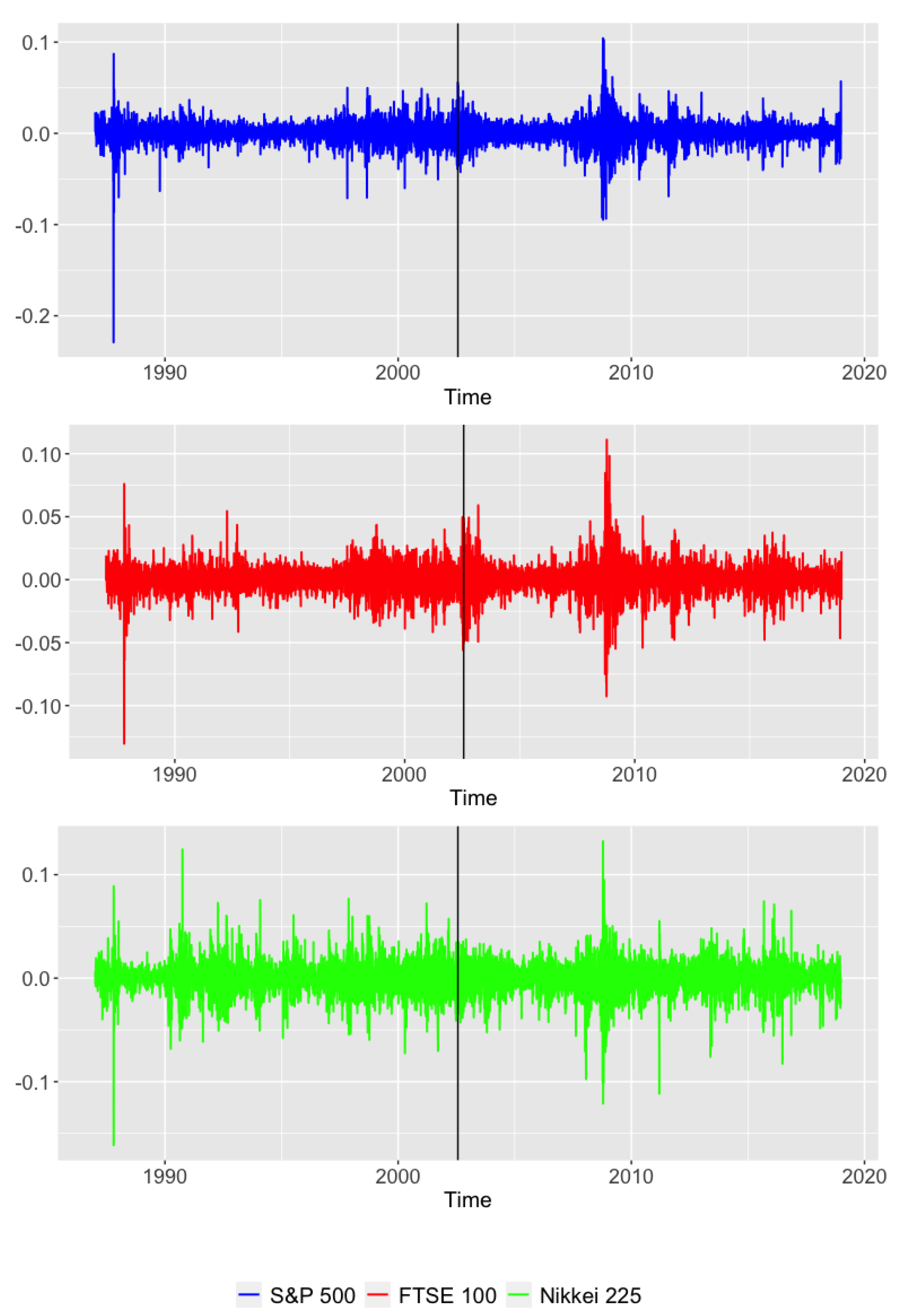
5.2. The Considered Data

To analyze the effects of the dotcom bubble in the global economy, we considered three well-known stock market indexes, which are briefly described below.
  • S&P 500. This index comprises 505 common stocks issued by 500 large-cap companies and traded on stock exchanges in the United States. The S&P 500 gives weights to the companies according to their market capitalization.
  • FTSE 100. This market index includes the 100 companies listed in the London Stock Exchange with the highest market capitalization. It is also a weighted index with weights depending on the market capitalization of the different firms.
  • Nikkei 225. This index is a price-weighted, stock market index for the Tokyo Stock Exchange. It measures the performance of 225 large, publicly owned companies in Japan from a wide array of industry sectors.
We focus on the trivariate time series formed by the daily stock prices of the three previous indexes. The data were sourced from the finance section of the Yahoo website (https://es.finance.yahoo.com, accessed on 20 July 2021). As our goal is to determine whether the dotcom bubble distorted the global market behavior, we split this MTS into two separate periods: before and after the bubble-burst period. To this end, we consider the periods from 1987 to 2002 and from 2003 to 2018. In addition, we only select dates corresponding to trading days for the three indexes and forming two periods of the same length. Based on these considerations, the first period covers the simultaneous trading days from 2 January 1987 to 25 July 2002, and the second period includes the simultaneous trading days from 26 July 2002 to 28 December 2018. In this way, each MTS is constituted by 3928 daily observations.
Since the series of closing prices are not stationary in mean, we proceed to take the first difference of the natural logarithm of the original values, thus obtaining series of so-called daily returns, which are depicted in Figure 1. The new series exhibit common characteristics of financial time series, so-called “stylized facts”, as heavy tails, volatility clustering, and leverage effects.
Two MTS were constructed by considering simultaneously the three UTS in Figure 1 before and after the dotcom bubble crash (vertical line). Then, the equality of the generating processes of both MTS was checked using the bootstrap tests proposed throughout the manuscript based on B = 500 bootstrap replicates.

5.3. Results

The p-values obtained by means of the methods MBB and SB were all 0. Therefore, both bootstrap techniques indicate rejection of the null hypothesis at any reasonable significance level. This suggests that the whole MTS exhibits a different dependence structure in each of the considered periods. A direct implication of this fact could be that the dotcom bubble crash in the early 2000s provoked a permanent change in the behavior of the global economy.

6. Conclusions

In this work, we addressed the problem of testing the equality of the stochastic processes generating two multivariate time series. For that purpose, we first defined a distance measure between multivariate processes based on comparing the quantile cross-spectral densities, called d Q C D . Then, two tests considering a proper estimate of this dissimilarity ( d ^ Q C D ) were proposed. Both approaches are based on bootstrap techniques. Their behavior under the null and the alternative hypotheses was analyzed through a simulation study. The techniques were also used to answer the question regarding whether or not the dotcom bubble crash of the 2000s affected global market behavior.

Author Contributions

Conceptualization, Á.L.-O. and J.A.V.; methodology, Á.L.-O. and J.A.V.; software, Á.L.-O.; writing—review and editing, Á.L.-O. and J.A.V. All authors have read and agreed to the published version of the manuscript.

Funding

This research has been supported by MINECO (MTM2017-82724-R and PID2020-113578RB-100), the Xunta de Galicia (ED431C-2020-14), and “CITIC” (ED431G 2019/01).

Institutional Review Board Statement

Not applicable.

Informed Consent Statement

Not applicable.

Data Availability Statement

Not applicable.

Acknowledgments

The authors thank ITISE 2022 organisers for allowing them to submit this paper to the proceedings.

Conflicts of Interest

The authors declare no conflict of interest.

References

  1. Liao, T.W. Clustering of time series data—A survey. Pattern Recognit. 2005, 38, 1857–1874. [Google Scholar] [CrossRef]
  2. Wu, J.; Yao, L.; Liu, B. An overview on feature-based classification algorithms for multivariate time series. In Proceedings of the 2018 IEEE 3rd International Conference on Cloud Computing and Big Data Analysis (ICCCBDA), Chengdu, China, 20–22 April 2018; pp. 32–38. [Google Scholar]
  3. Blázquez-García, A.; Conde, A.; Mori, U.; Lozano, J.A. A Review on outlier/Anomaly Detection in Time Series Data. ACM Comput. Surv. (CSUR) 2021, 54, 1–33. [Google Scholar] [CrossRef]
  4. Tsay, R.S. Nonlinearity tests for time series. Biometrika 1986, 73, 461–466. [Google Scholar] [CrossRef]
  5. Lafuente-Rego, B.; Vilar, J.A. Clustering of time series using quantile autocovariances. Adv. Data Anal. Classif. 2016, 10, 391–415. [Google Scholar] [CrossRef]
  6. López-Oriona, Á.; Vilar, J.A. Quantile cross-spectral density: A novel and effective tool for clustering multivariate time series. Expert Syst. Appl. 2021, 185, 115677. [Google Scholar] [CrossRef]
  7. Preuß, P.; Hildebrandt, T. Comparing spectral densities of stationary time series with unequal sample sizes. Stat. Probab. Lett. 2013, 83, 1174–1183. [Google Scholar] [CrossRef] [Green Version]
  8. Dette, H.; Kinsvater, T.; Vetter, M. Testing non-parametric hypotheses for stationary processes by estimating minimal distances. J. Time Ser. Anal. 2011, 32, 447–461. [Google Scholar] [CrossRef] [Green Version]
  9. Jentsch, C.; Pauly, M. Testing equality of spectral densities using randomization techniques. Bernoulli 2015, 21, 697–739. [Google Scholar] [CrossRef]
  10. López-Oriona, Á.; Vilar, J.A.; D’Urso, P. Quantile-based fuzzy clustering of multivariate time series in the frequency domain. Fuzzy Sets Syst. 2022, 443, 115–154. [Google Scholar] [CrossRef]
  11. López-Oriona, Á.; D’Urso, P.; Vilar, J.A.; Lafuente-Rego, B. Quantile-based fuzzy C-means clustering of multivariate time series: Robust techniques. arXiv 2021, arXiv:2109.11027. [Google Scholar]
  12. Lopez-Oriona, A. Spatial weighted robust clustering of multivariate time series based on quantile dependence with an application to mobility during COVID-19 pandemic. IEEE Trans. Fuzzy Syst. 2021, 1. [Google Scholar] [CrossRef]
  13. Kunsch, H.R. The jackknife and the bootstrap for general stationary observations. Ann. Stat. 1989, 17, 1217–1241. [Google Scholar] [CrossRef]
  14. Liu, R.Y.; Singh, K. Moving blocks jackknife and bootstrap capture weak dependence. Explor. Limits Bootstrap 1992, 225, 248. [Google Scholar]
  15. Politis, D.N.; Romano, J.P. The stationary bootstrap. J. Am. Stat. Assoc. 1994, 89, 1303–1313. [Google Scholar] [CrossRef]
  16. Baruník, J.; Kley, T. Quantile coherency: A general measure for dependence between cyclical economic variables. Econom. J. 2019, 22, 131–152. [Google Scholar] [CrossRef] [Green Version]
  17. Kley, T.; Volgushev, S.; Dette, H.; Hallin, M. Quantile spectral processes: Asymptotic analysis and inference. Bernoulli 2016, 22, 1770–1807. [Google Scholar] [CrossRef]
  18. Engle, R. Dynamic conditional correlation: A simple class of multivariate generalized autoregressive conditional heteroskedasticity models. J. Bus. Econ. Stat. 2002, 20, 339–350. [Google Scholar] [CrossRef]
  19. Hall, P.; Horowitz, J.L.; Jing, B.Y. On blocking rules for the bootstrap with dependent data. Biometrika 1995, 82, 561–574. [Google Scholar] [CrossRef]
  20. Geier, B. What Did We Learn from the Dotcom Stock Bubble of 2000. Available online: https://time.com/3741681/2000-dotcom-stock-bust/ (accessed on 20 July 2021).
  21. Clarke, T. e Dot-Com Crash of 2000–2002. Available online: https://moneymorning.com/2015/06/12/the-dot-com-crash-of-2000-2002/ (accessed on 20 July 2021).
  22. Morris, J.J.; Alam, P. Value relevance and the dot-com bubble of the 1990s. Q. Rev. Econ. Financ. 2012, 52, 243–255. [Google Scholar] [CrossRef]
Figure 1. Daily returns of the S&P 500 (top panel), FTSE 100 (middle panel), and Nikkei 225 (bottom panel) stock market indexes from 2 January 1987 to 28 December 2018. The vertical line indicates the end of the dotcom bubble burst.
Engproc 18 00038 g001
Table 1. Simulated rejection probabilities under the null hypothesis for α = 0.05 .
TMethodScenario
123
500MBB0.0800.0700.080
SB0.0550.0550.050
1000MBB0.0700.0950.130
SB0.0400.0600.060
Table 2. Simulated rejection probabilities of the bootstrap tests under several alternative hypotheses determined by the deviation parameter δ .
TMethodScenario 1Scenario 2Scenario 3
δ δ δ
0 . 1 0 . 2 0 . 3 0 . 2 0 . 4 0 . 6 0 . 4 0 . 8 1 . 2
100MBB0.1600.5750.9800.5400.7750.9900.0800.3950.950
SB0.1000.4650.9600.3250.6900.9100.0550.2300.870
200MBB0.1850.7900.9950.7800.92510.1850.7251
SB0.0950.6950.9900.6250.8850.9850.0800.4550.965
300MBB0.2250.83510.8850.99010.2550.8401
SB0.1300.77010.8050.95510.1550.6951
Publisher’s Note: MDPI stays neutral with regard to jurisdictional claims in published maps and institutional affiliations.

