Estimation of Continuous Distribution of Iterated Fission Probability Using an Artificial Neural Network with Monte Carlo-Based Training Data

Abstract

The Monte Carlo neutron transport method is used to accurately estimate various quantities, such as k-eigenvalue and integral neutron flux. However, in the case of estimating a distribution of a desired quantity, the Monte Carlo method does not typically provide continuous distribution. Recently, the functional expansion tally (FET) and kernel density estimation (KDE) methods have been developed to provide a continuous distribution of a Monte Carlo tally. In this paper, we propose a method to estimate a continuous distribution of a quantity in all phase-space variables using a fully connected feedforward artificial neural network (ANN) model with Monte Carlo-based training data. As a proof of concept, a continuous distribution of iterated fission probability (IFP) was estimated by ANN models in two distinct fissile systems. The ANN models were trained on the training data created using the Monte Carlo IFP method. The estimated IFP distributions by the ANN models were compared with the Monte Carlo-based data that include the training data. Additionally, the IFP distributions by the ANN models were also compared with the adjoint angular neutron flux distributions obtained with the deterministic neutron transport code PARTISN. The comparisons showed varying degrees of agreement or discrepancy; however, it was observed that the ANN models learned the general trend of the IFP distributions from the Monte Carlo-based training data.

1. Introduction

The Monte Carlo neutron transport method offers an accurate estimation of various quantities of interest such as k-eigenvalue and neutron flux or reaction rate integrated over a phase-space region. In order to estimate a distribution of a desired quantity (e.g., neutron flux and reaction rate) over the phase-space domain of a problem, one mostly needs to divide the phase-space domain into a number of bins (e.g., mesh) and tally the quantity in each bin, since the Monte Carlo method does not typically provide a continuous distribution. With this method, it becomes challenging to obtain the desired distribution over a finer bin structure because the uncertainty of the tally in a small bin becomes large due to a smaller number of events contributing to the bin. On the other hand, a few methods to estimate a continuous distribution of a desired quantity over the phase-space domain of a problem have been studied. In particular, kernel density estimation (KDE) and functional expansion tally (FET) methods have been developed and applied to estimate the continuous spatial distribution of neutron flux [1,2,3,4,5]. Both methods provide an estimation of a continuous distribution and corresponding uncertainty of a tally during a Monte Carlo calculation. In particular, the FET method has recently been used for estimating spatial distributions of neutron flux and power density [6,7,8].

However, the FET and KDE methods have been applied to one- to three-dimensional spatial distribution problems; application of the KDE and FET methods to problems of estimating a continuous distribution of a Monte Carlo tally in all space, energy, and direction variables is scarce or has not yet appeared in the literature, to the best of the authors’ knowledge. Consequently, the estimation of a continuous distribution of a variable in all phase-space variables still remains a challenging problem. This motivated the authors to explore an alternative method for estimating a continuous distribution of variables in space, energy, and direction.

In this paper, we propose a fully connected feedforward artificial neural network (ANN) model-based method for estimating a continuous distribution of a quantity in space, energy, and direction from Monte Carlo-based training data. An ANN model learns, albeit approximately, a continuous distribution from discrete data via supervised learning. As a proof of concept, we consider the estimation of a continuous distribution of iterated fission probability (IFP), which is a quantity proportional to adjoint angular neutron flux, via an ANN model in a given fissile system from Monte Carlo-based training data. The IFP was selected in this study because the algorithm to calculate IFP is more suitable for creating data for training an ANN model in a given system; the algorithm provides an estimation of IFP at a desired phase-space location. The proposed ANN model-based method estimates a continuous distribution from data after a Monte Carlo calculation is finished, in contrast to the KDE and FET methods, which can estimate the continuous distribution during the Monte Carlo calculation. Furthermore, at this preliminary stage, the proposed ANN model-based method does not provide an estimation of uncertainty on an obtained continuous distribution.

The IFP denoted as $R\left(\mathit{r},E,\mathit{\Omega }\right)$ at phase-space location $\mathit{P}\equiv \left(\mathit{r},E,\mathit{\Omega }\right)$ represents an asymptotic population due to a source neutron introduced at that location in a given system. It was shown [9,10,11] that IFP is proportional to a fundamental mode of adjoint angular neutron flux. Since IFP distribution is governed by an integral equation that cannot be solved directly in general, it is estimated via a Monte Carlo neutron transport method. The methods to estimate IFP in a forward Monte Carlo eigenvalue neutron transport calculation have been developed [9,10], implemented in Monte Carlo neutron transport codes, and used for various applications [12,13,14,15,16,17,18,19,20,21,22]. Although unknown, there must be a function describing the $R\left(\mathit{r},E,\mathit{\Omega }\right)$ distribution in a given system. Let us assume that the unknown function is $f_t$ such that $R=f_t\left(r,E,\Omega \right)$ in a given system, which is characterized by its geometry, material composition, temperature, etc. The function $f_t$ maps from phase-space location $\mathit{P}$ to its corresponding IFP value $R$, that is, $f_t:{\mathbb{R}}^7\to \mathbb{R}$. This unknown function can be learned, at least approximately, by an ANN model, which is trained via supervised learning on data created by the Monte Carlo method. Once an ANN model is trained successfully on the data in a given system, it can then be used to estimate an IFP at any phase-space location in the system, i.e., it can provide a continuous IFP distribution in the system.

In the previous study [23], we showed the preliminary approximation of the IFP distribution via an ANN model for the first time using the Godiva system. In that study, the data were mostly produced according to the fission neutron distribution in the system. In other words, the spatial position was sampled from fission sites in the system, energy was sampled from the fission neutron spectrum, and direction was sampled from isotropic distribution. With these sampling distributions, a majority of the data was around the peak of the fission neutron spectrum, reducing the amount of data for other energy regions. It was shown that although the ANN model learned the IFP distribution approximately, it failed to learn the dependence of resonance-like peaking of the IFP distribution on the energy variable. In contrast to the previous study, we consider applying ANN models for estimating continuous IFP distributions in two distinct fissile systems in this study: the fast spectrum Godiva core and the thermal spectrum simplified STACY core. Furthermore, in the current study, the data are produced via arbitrary sampling distributions intended for enhancing the training of ANN models.

The purpose of this paper is to show the proof of concept of the ANN model-based method for estimating a continuous distribution of a quantity from Monte Carlo-based training data. To this end, an estimation of a continuous distribution of IFP via ANN models in two distinct fissile systems in terms of neutron spectrum is considered. The paper is structured as follows. In Section 2, the Monte Carlo method for estimating an IFP at a given phase-space location is described. The procedure to create discrete data is given in Section 3 for the Godiva and simplified STACY cores. Section 4 presents the considered ANN models, their training, and estimated IFP distributions by the ANN models. The estimated distributions by the selected ANN models are compared to the Monte Carlo-based data that include the training data in Section 4. Furthermore, the comparisons between the estimated IFP distributions by the selected ANN models and the adjoint angular neutron flux distributions by the deterministic neutron transport code PARTISN are provided. The concluding remarks are given in Section 5.

2. Iterated Fission Probability Method

In this section, the estimation of an IFP at a given phase-space location in a given system using the Monte Carlo neutron transport method, which is based on the IFP calculation method by Kiedrowski et al. [9], is presented. The theoretical discussion of the IFP method and the proportionality of IFP to adjoint angular neutron flux can be found in the references [9,10,11].

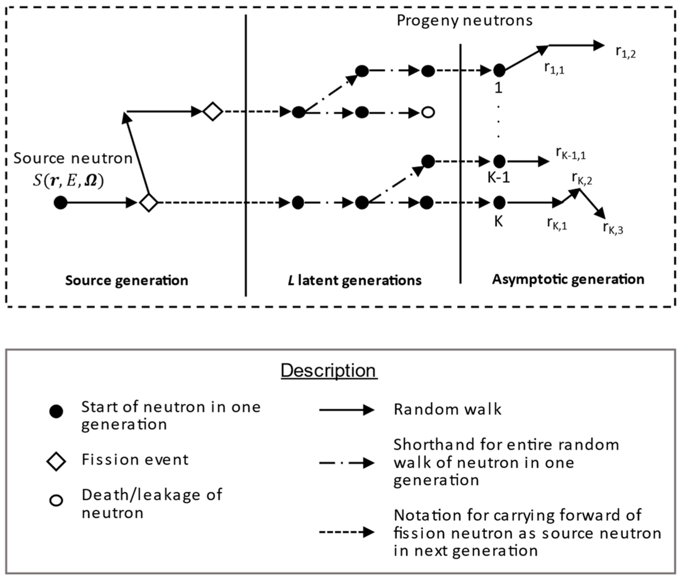
In the IFP method by Kiedrowski et al., entire active cycles (generations) of a forward Monte Carlo eigenvalue calculation are divided into non-overlapping uniform intervals called blocks. Each block consists of an original generation, latent generation(s), and an asymptotic generation. The original generation is located at the beginning of the block and is followed by L latent generation(s). The last generation in the block is the asymptotic generation. In each block, the IFP for each progenitor neutron in the original generation is estimated as a total fission neutron production by all of its progeny neutrons in the asymptotic generation. A sufficient number of latent generations allows the progenies of the progenitor neutron to converge to their asymptotic population.

Kiedrowski’s method is generally designed for estimating adjoint-weighted quantities such as kinetic parameters and sensitivity coefficients in steady-state fissile systems; hence, it is implemented for forward Monte Carlo eigenvalue calculations. Consequently, phase-space locations of source (progenitor) neutrons are sampled from fission sites: energy is sampled from a fission neutron spectrum, the spatial position is set to the fission site, and direction is sampled from isotropic distribution. On the contrary, in this study, we are interested only in the estimation of IFP itself; a forward Monte Carlo eigenvalue problem is not needed, and source neutrons can be sampled arbitrarily as in a fixed-source Monte Carlo calculation.

Figure 1 shows the general procedure, which is based on Kiedrowski’s method, for estimating an IFP at a given phase-space location in this study with an example. A source neutron (equivalent to a progenitor neutron in Kiedrowski’s method) is introduced at the phase-space location $\left(\mathit{r},E,\mathit{\Omega }\right)$ and is tracked in the source generation. Fission neutrons (progeny neutrons in Kiedrowski’s method) caused by the source neutron are then tracked over the next L latent generations. Eventually, an IFP is estimated as a total fission neutron production by all progeny neutrons in the asymptotic generation as below using the track-length estimator.

$$R\left(\mathit{r},E,\Omega \right)={{\displaystyle \sum }}_{k=1}^K{{\displaystyle \sum }}_{m=1}^{M_k}{r}_{k,m}={{\displaystyle \sum }}_{k=1}^K{{\displaystyle \sum }}_{m=1}^{M_k}\nu {\Sigma }_f{w}_{k,m}{l}_{k,m},$$

(1)

where $k$ denotes a progeny neutron index in the asymptotic generation, $m$ denotes the m-th collision of a progeny neutron, $K$ is the total number of progeny neutrons in the asymptotic generation, $M_k$ is the total number of interactions (collision or surface crossing) by a progeny neutron $k$, $\nu {\Sigma }_f$ is fission neutron production at an interaction (collision or surface crossing) site, and $w_{k,m}$ and $l_{k,m}$ are the weight and track length of progeny neutron $k$ at its $m$-th interaction, respectively.

The procedure described in Equation (1) and Figure 1 estimates an IFP for one random sample at a given phase-space location. For the purpose of training ANN models later in this paper, we calculate the mean IFP at a given phase-space location. A source neutron at phase-space location $\left(\mathit{r},E,\Omega \right)$ is cloned $N_c$ times and each clone is given a unique initial random number to estimate the mean IFP as

$$\overline{R}\left(\mathit{r},E,\Omega \right)=\frac{1}{N_c}{{\displaystyle \sum }}_{i=1}^{N_c}R\left(\mathit{r},E,\Omega \left|{\xi }_i\right.\right),$$

(2)

where ${\xi }_i$ is the initial random number for the $i$-th clone.

The Monte Carlo IFP method described in this section has been newly implemented in continuous-energy Monte Carlo neutron transport solver Solomon [24]. In the rest of this paper, the Monte Carlo IFP method described in this section and the Solomon solver are used interchangeably.

3. Creation of Monte Carlo-Based Data

3.1. General Approach

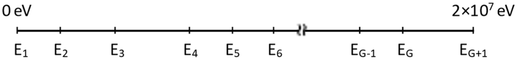
In order to create data for a given system, a phase-space domain of the system needs to be sampled according to some sampling distributions. In general, all variables (position, energy, and direction) can be sampled from a uniform distribution in the domain. Typically, the geometrical domain of a fissile system is limited, i.e., on the order of 10⁰ m, and the angular domain is bounded in [−1.0, 1.0] for each component of the direction. On the other hand, the energy domain spans over the range [0.0, 2 × 10⁷] eV. If energy is sampled from a uniform distribution in the entire range, a majority of the data then will consist of samples with high energy. Alternatively, if energy is sampled uniformly on a logarithmic scale in the entire range, then a majority of the data consists of neutrons with energy less than 1.0 eV. In order to include samples from various energy regions more equally, we consider dividing the entire range into G intervals and sampling from a uniform distribution in each interval as illustrated in Figure 2. Furthermore, an arbitrary number of samples can be drawn in each interval. This division facilitates a more flexible sampling and improves the overall sampling of various energy ranges; however, the boundaries of each energy interval need to be decided. In the next two sections, we will introduce such energy structures for the Godiva and simplified STACY cores. It should be noted that an energy structure is only needed for creating the data containing discrete samples; an IFP distribution to be learned by an ANN model from the data is continuous and generally independent of the energy structure provided that the training is successful.

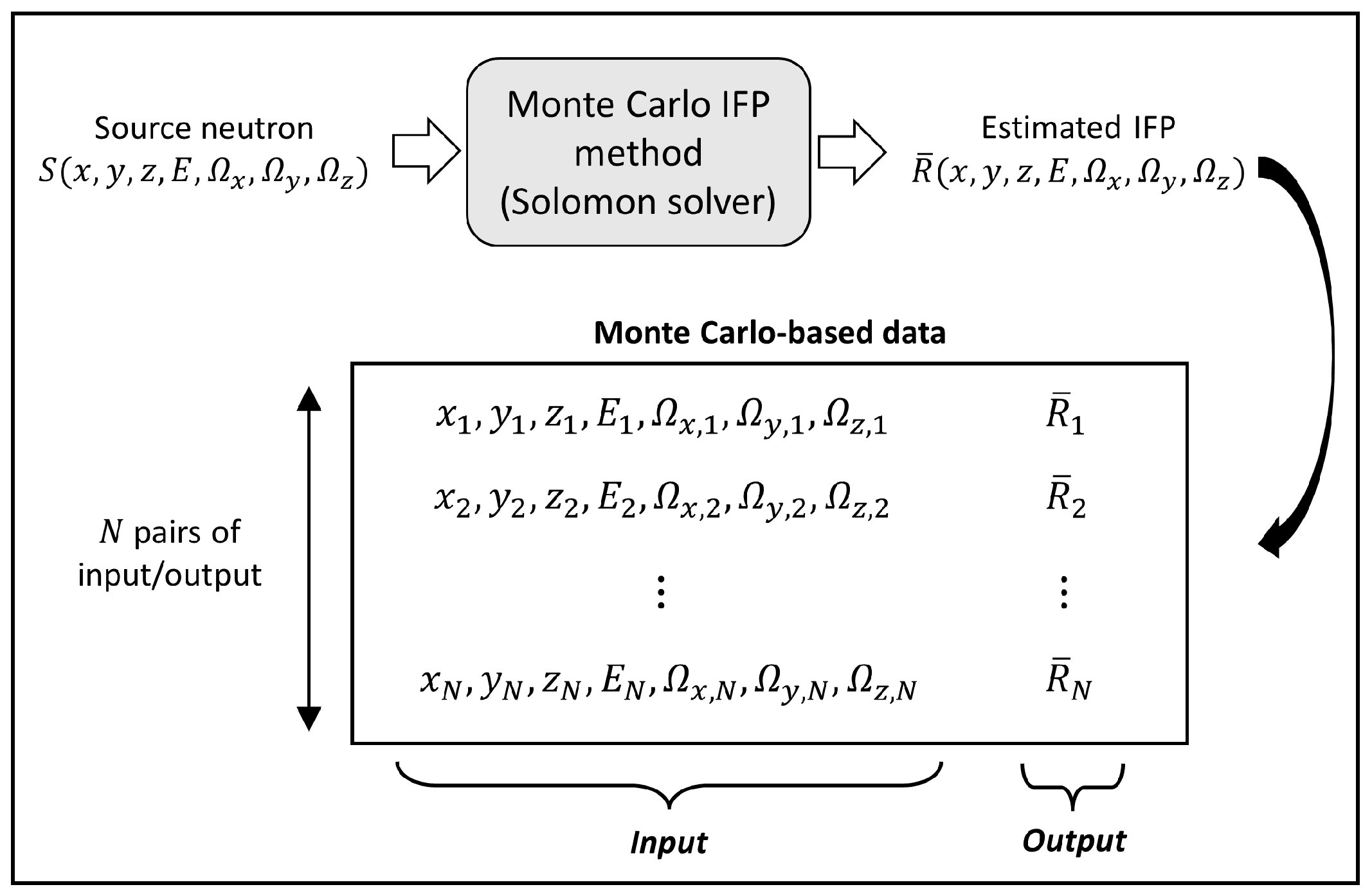
With the described sampling procedure, the spatial position, energy, and direction of each source neutron are sampled randomly from uniform distributions in each energy interval. An IFP corresponding to a given source neutron is then estimated via the Solomon solver as discussed in Section 2. Data in a given system then can be created by storing the phase-space location (input) of a source neutron and the estimated IFP (output) as illustrated in Figure 3. An ANN model can be trained to estimate a continuous distribution of IFP via supervised learning from such data containing discrete phase-space locations and IFP pairs.

It should be noted that the phase-space location sampling procedure described in this section (and in Section 3.2 and Section 3.3) is only necessary for the estimation of IFP distribution. In the case of other quantities such as forward neutron flux and reaction rates, phase-space locations would be sampled according to collision and surface crossing events during a Monte Carlo calculation. Data then would be created by storing phase-space locations of the events and corresponding estimations of a quantity.

3.2. Data in Godiva Core

The Godiva [25] is a bare spherical core of highly enriched metallic uranium with about 94.73 wt.% ²³⁵U. Its radius is 8.741 cm and its physical density is 18.74 g/cm³. The atomic number densities of ²³⁴U, ²³⁵U, and ²³⁸U are 4.9184 × 10⁻⁴, 4.4994 × 10⁻², and 2.4984 × 10⁻³ atoms × barn⁻¹ × cm⁻¹, respectively.

The phase-space domain of the Godiva core is bounded in [−8.741, 8.741] cm for space, [−1.0, 1.0] for angular component, and [0.0, 2.0 × 10⁷] eV for energy. As described in the previous section, we divide the energy range into a number of intervals to improve the sampling. Although the energy structure of such division can be decided arbitrarily, we used the 73-group energy structure from the SLAROM-UF code [26] in order to make a comparison of an estimated IFP distribution by an ANN model and adjoint angular neutron flux distribution by a deterministic code, in which the same energy group structure is used, simpler. The 73-group energy structure is the smallest fine group structure provided by the SLAROM-UF code. The number of clones was set to 100. In each energy interval, 8 × 10⁴ samples were created using the IFP method in the Solomon solver, giving a total of 5.84 × 10⁶ samples in the data. The number of latent generations in the IFP method was set to 10, a value recommended for most problems.

3.3. Data in Simplified STACY Core

The simplified STACY [27] is an infinite cylindrical core of enriched uranyl nitrate solution surrounded by a light water reflector. The radius of the inner infinite cylinder containing the uranyl nitrate solution is 22.0 cm and the outer radius is 23.0 cm, giving the light water reflector a thickness of 1.0 cm.

Table 1. Atomic number densities of simplified STACY core.

Material	Nuclide	Atomic Density (atoms × barn−1 × cm−1)
Fuel solution	235U	7.92122 × 10−5
	238U	7.06258 × 10−4
	1H	5.69525 × 10−2
	14N	2.87772 × 10−3
	16O	3.80270 × 10−2
Light water reflector *	1H	6.66566 × 10−2
	16O	3.33283 × 10−2

* Free gas treatment is used for ¹H in Solomon.

lists the atomic number densities of the constituent nuclides.

The data in the simplified STACY core are created similarly to those in the case of the Godiva core. The phase-space domain of the simplified STACY core is bounded in [−23.0, 23.0] cm for X- and Y-axis, [−∞, ∞] for Z-axis, [−1.0, 1.0] for angular component, and [0.0, 2.0 × 10⁷] eV in energy. The range in the Z-axis is sampled in [−50.0, 50.0]; however, this does not affect the IFP distribution at all as it does not vary in the Z-axis. The energy is sampled from the uniform distribution in each energy interval as described in Section 3.1. In this study, we used the 107-group energy structure from the SRAC code [28] in order to make a comparison with adjoint angular neutron flux distribution by a deterministic code later, in which the same energy structure is used. The 107-group structure is the only energy structure provided by the SRAC code. Furthermore, it should be noted that the 107-group energy structure is bounded in [0.0, 1.0 × 10⁷] eV, meaning that with the created data, the continuous distribution of IFP in this range is supposed to be estimated by ANN models. The number of clones was set to 100. In total, the data contain 2.14 × 10⁶ samples created via the IFP method in Solomon; in other words, 2 × 10⁴ samples were drawn in each energy interval. The number of latent generations in the IFP method was set to 10.

4. Estimation of Continuous IFP Distribution via ANN Model

4.1. Descriptions of ANN Models and Training

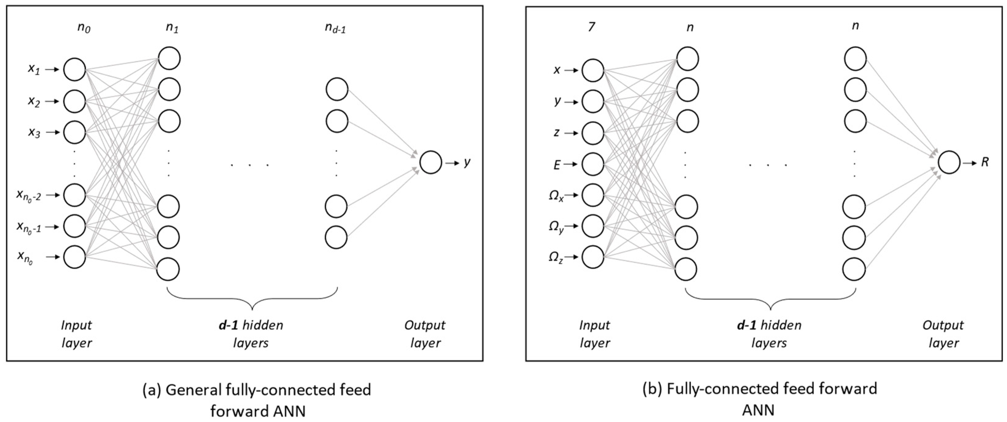
A fully connected feedforward artificial neural network [29] (ANN) with a single real-valued output is considered in this work. Figure 4a shows such an ANN. It consists of an input layer, $d-1$ layers called hidden layers, and an output layer. The number of neurons in each hidden layer is a model hyperparameter that needs to be decided arbitrarily or via hyperparameter search. The number of possibilities of making ANN models with a different number of neurons in each hidden layer grows exponentially with the depth $d$. In order to simplify the hyperparameter search, we consider ANNs in which the number of neurons in each hidden layer is the same, as shown in Figure 4b, where $n$ is the number of neurons in each hidden layer and is referred to as the width of the network. Consequently, only the optimal values of width and depth need to be searched for.

In order to find the optimal depth and width of the network for each system, we performed a random search [30]. Ten combinations of width and depth were sampled randomly from the ranges (7, 42) for width and (5, 21) for depth; these ranges were partly identified as suitable in the previous study [23]. The sampled combinations are given in

Table 2. Combinations of width and depth resulted from random search.

ANN Model Identification	$\mathbf{Width}\mathbf{,} \mathit{n}$	$\mathbf{Depth}\mathbf{,} \mathit{d}$
ANN-1	41	12
ANN-2	30	14
ANN-3	24	8
ANN-4	18	17
ANN-5	13	20
ANN-6	23	9
ANN-7	20	7
ANN-8	8	5
ANN-9	19	6
ANN-10	17	20

. Consequently, ten ANN models were created to be trained for each system. The rectified linear unit (ReLU) function is used as an activation function for each hidden layer.

In addition to the model hyperparameters, there are algorithmic hyperparameters related to the training of an ANN model such as a learning rate and batch size (batch size is the number of training samples used for updating model parameters). In this work, we set the learning rate to 0.001, which is common in practice. The batch size was set to about 1% of the total number of samples in the data.

To train an ANN model, a measure of the performance of the ANN model training is needed for optimization purposes. Such a measure is called a cost function. As the current task of estimating an IFP distribution via an ANN model is a non-linear regression task, a commonly used cost function named Mean Squared Error (MSE), defined in Equation (3), is used in this work.

$$J\left(\mathit{\theta }\right)\equiv MSE=\frac{1}{N}{{\displaystyle \sum }}_{i=1}^N{\left({\overline{R}}_i-{\widehat{R}}_i\right)}^2=\frac{1}{N}{{\displaystyle \sum }}_{i=1}^N{\left({\overline{R}}_i-f\left({\mathit{r}}_{\mathit{i}},E_i,{\mathit{\Omega }}_{\mathit{i}}\left|\mathit{\theta }\right.\right)\right)}^2,$$

(3)

where $\mathit{\theta }$ is the parameters of the ANN model, ${\overline{R}}_i$ is the IFP corresponding to $i$-th input in the data (i.e., the IFP calculated by the Solomon solver via Equation (2)), ${\widehat{R}}_i$ is the IFP estimation by the ANN model for the $i$-th input, and $N$ is the number of samples in the data. The parameters $\mathit{\theta }$, which consist of the weights and biases, were initialized randomly in the range [−2.0, 2.0] in this study.

The constructed ANN models are then trained on the data using the gradient descent algorithm named Adam optimizer [31], which is a well-known stochastic gradient descent algorithm. The gradient descent algorithm minimizes the cost function so that an ANN model learns the underlying IFP distribution, albeit approximately, from the data. To help ANN models generalize well and learn the underlying IFP distribution without overfitting the training data, the early stopping technique [32] is used.

Before training, the data are transformed using the power transformer [33], which tries to make each input variable have a normal distribution centered around 0 with unit variance, to improve the training in each system. The data in each system are then divided into training, validation, and test data with ratios of 0.67, 0.08, and 0.25, respectively; these ratios are common in machine learning applications.

4.2. Results and Discussion

4.2.1. Godiva Core

Ten ANN models constructed according to the widths and depths given in Table 2 have been trained on the training data.

Table 3. Training results of ANN models on Godiva data.

ANN Model	MSE
	Training	Validation	Test
ANN-1	2.6 × 10−1	2.7 × 10−1	2.7 × 10−1
ANN-2	2.6 × 10−1	2.6 × 10−1	2.6 × 10−1
ANN-3	2.5 × 10−1	2.5 × 10−1	2.5 × 10−1
ANN-4	2.8 × 10−1	2.9 × 10−1	2.9 × 10−1
ANN-5	2.7× 10−1	2.6 × 10−1	2.8 × 10−1
ANN-6	2.7 × 10−1	2.7 × 10−1	2.7 × 10−1
ANN-7	2.7 × 10−1	2.7 × 10−1	2.7 × 10−1
ANN-8	3.2 × 10−1	3.2 × 10−1	3.2 × 10−1
ANN-9	2.7 × 10−1	2.8 × 10−1	2.8 × 10−1
ANN-10	2.7 × 10−1	2.7 × 10−1	2.7 × 10−1

lists the training, validation, and test MSEs by each ANN model. It can be observed that MSEs by the different ANN models did not vary significantly, giving the maximum relative difference of about 22% between ANN-3 and ANN-8. Based on the training result, ANN-3 is selected as it provides the smallest test MSE among the ten ANN models. ANN-3 consists of 4585 parameters in total and 4201 of them are trainable parameters. The training time for ANN-3 was 1 hour on a typical desktop computer with Intel(R) Core(TM) i7 (1.4 GHz) CPU and 32GB RAM.

In order to compare the estimated IFP distribution by the selected ANN model with the Monte Carlo-based data by the Solomon solver (refer to Section 3.2), a group-wise IFP spectrum (i.e., mean IFPs over the energy structure) is considered because it is a commonly used distribution for comparison. The group-wise mean IFP is calculated simply as below.

$$R_g=\frac{1}{N_g}{{\displaystyle \sum }}_{E\in g}R\left(\mathit{r},E,\mathit{\Omega }\right),$$

(4)

where $R$ is the IFP by either the Solomon solver or the selected ANN model and $N_g$ is the number of samples that have energy belonging to group $g$. The IFPs by the selected ANN model are estimated at the same phase-space locations as the Solomon solver, which means the IFPs are estimated by the selected ANN model at the phase-space locations of all the data. The standard deviation of the mean IFP by the Solomon solver is estimated as

$${\sigma }_g=\sqrt{\frac{1}{N_g\left(N_g-1\right)}{{\displaystyle \sum }}_{E\in g}\left({\overline{R}}^2\left(\mathit{r},E,\mathit{\Omega }\right)-R_g^2\right)}.$$

(5)

Since only the shape of an IFP distribution is important, the IFP spectra by the selected ANN model and Solomon solver are further normalized to their respective integral values (i.e., ${{\displaystyle \sum }}_{g=1}^G{R}_g$) for a given energy structure with $G$ intervals. It should be noted that an energy structure used for making an IFP spectrum is arbitrary and not necessarily the same as the energy structures used for creating the data described in Section 3.

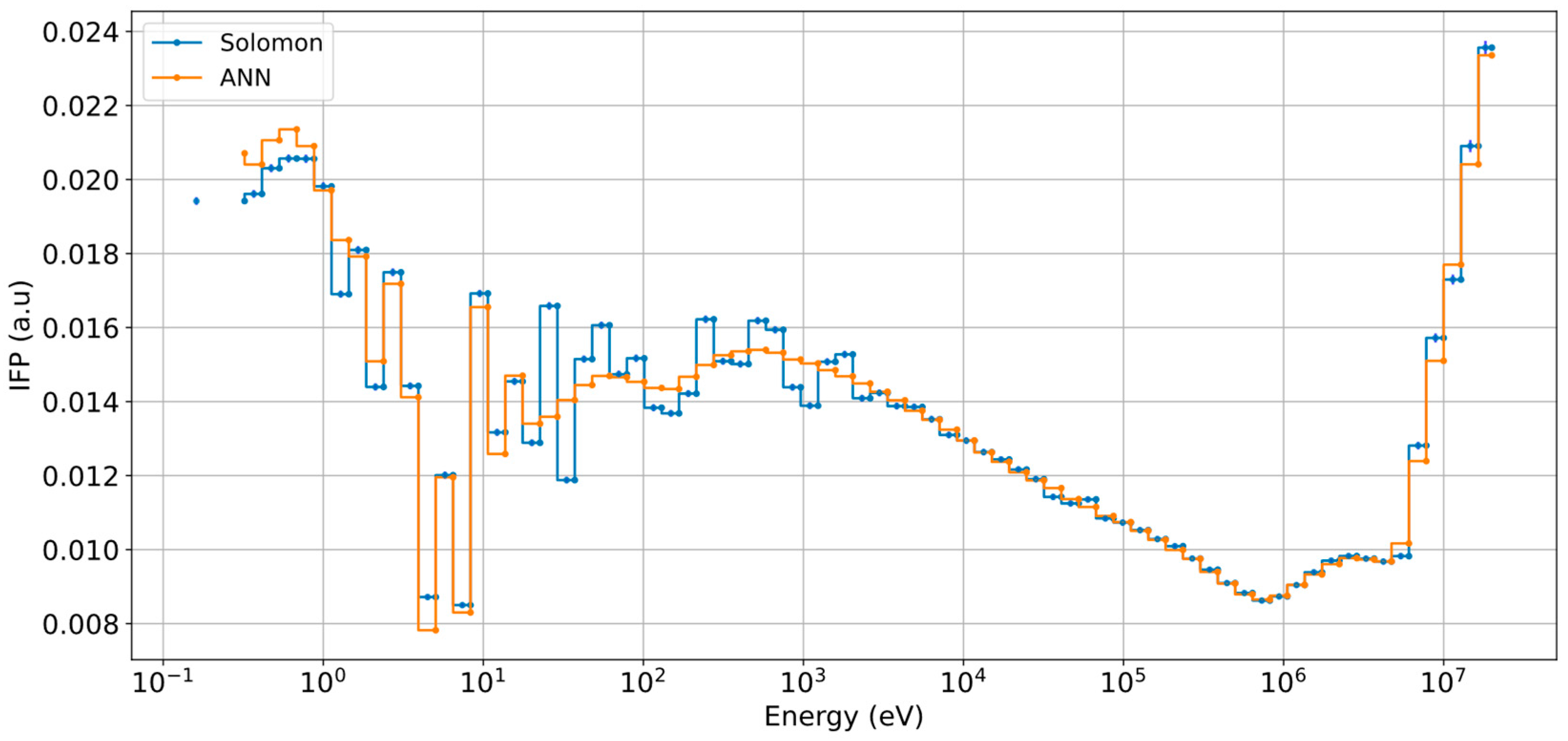
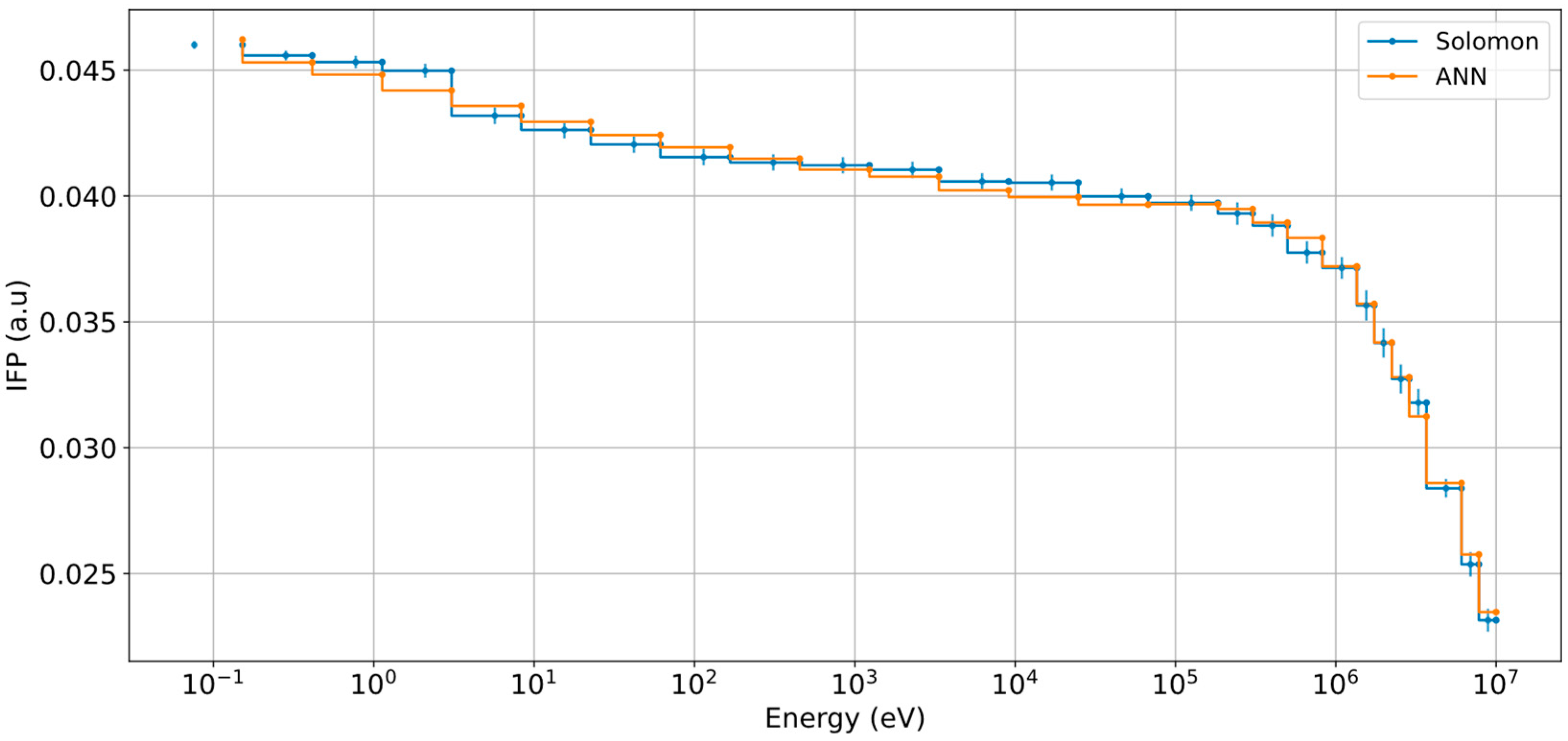
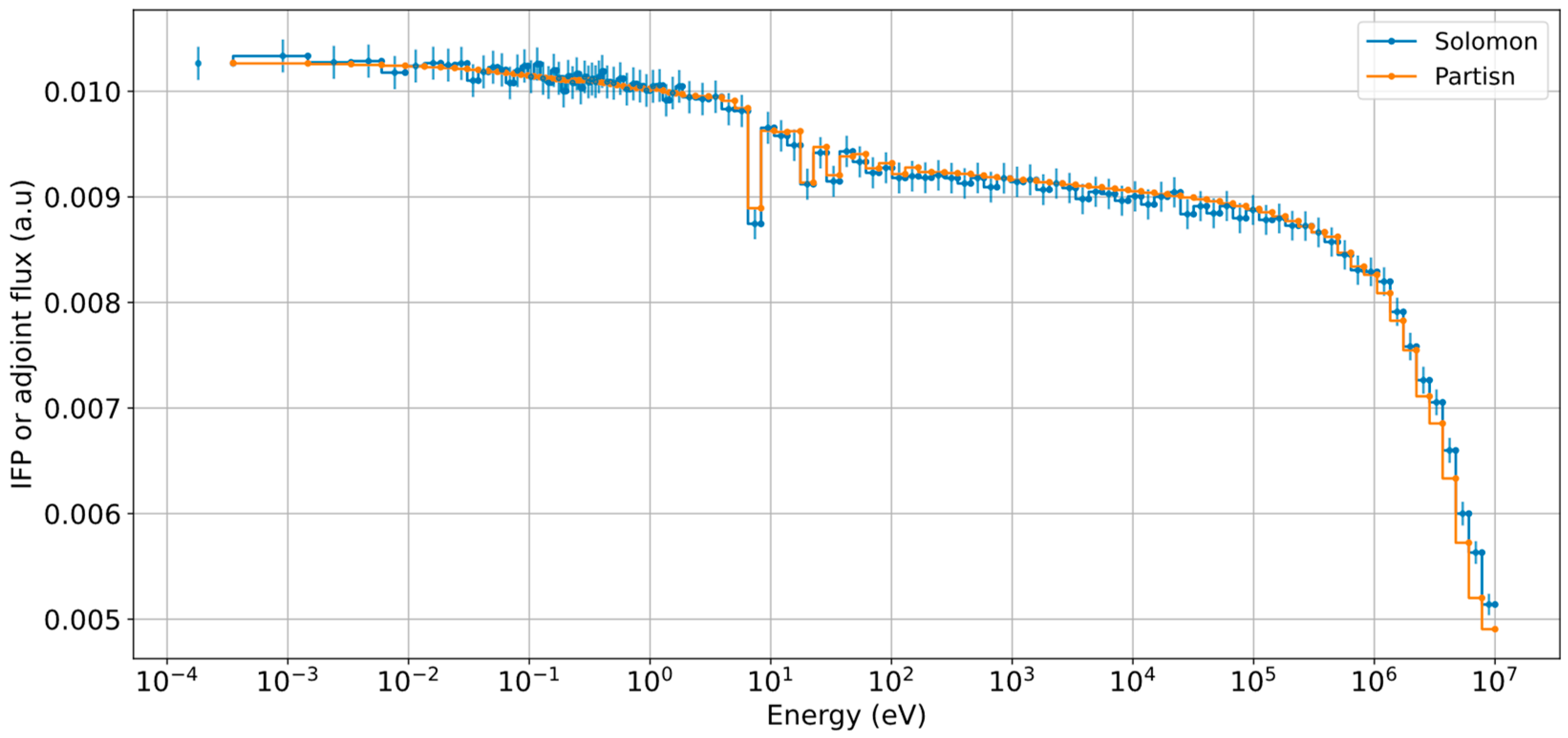
Figure 5 shows the group-wise IFP spectra by the Solomon solver and the selected ANN model using the SLAROM-UF-73g energy structure. It can be seen from Figure 5 that there are peak structures in the range [10⁰, 10⁴] eV related to the resonance cross-sections of ²³⁵U and ²³⁸U. The distribution by the ANN model showed only a part of this structure.

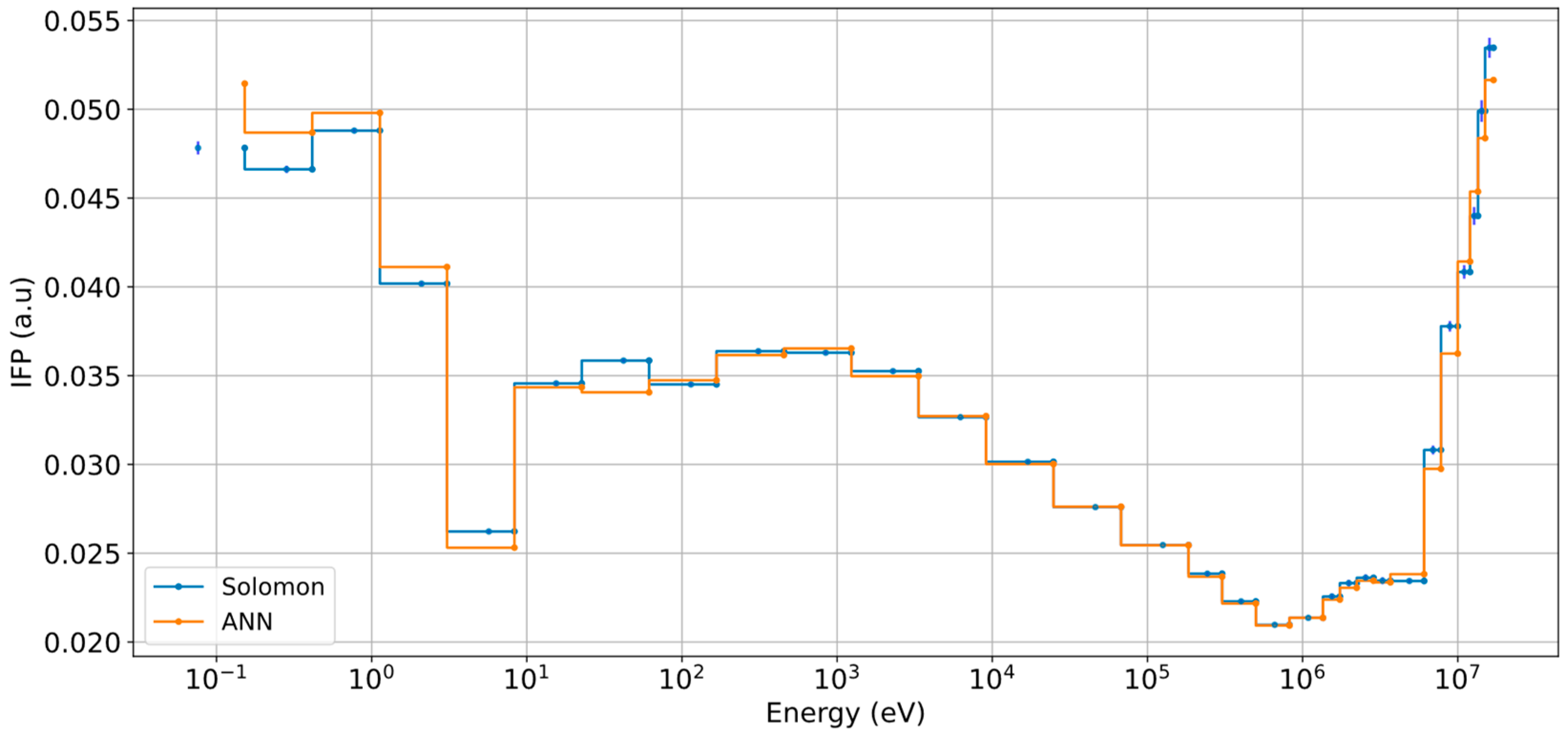
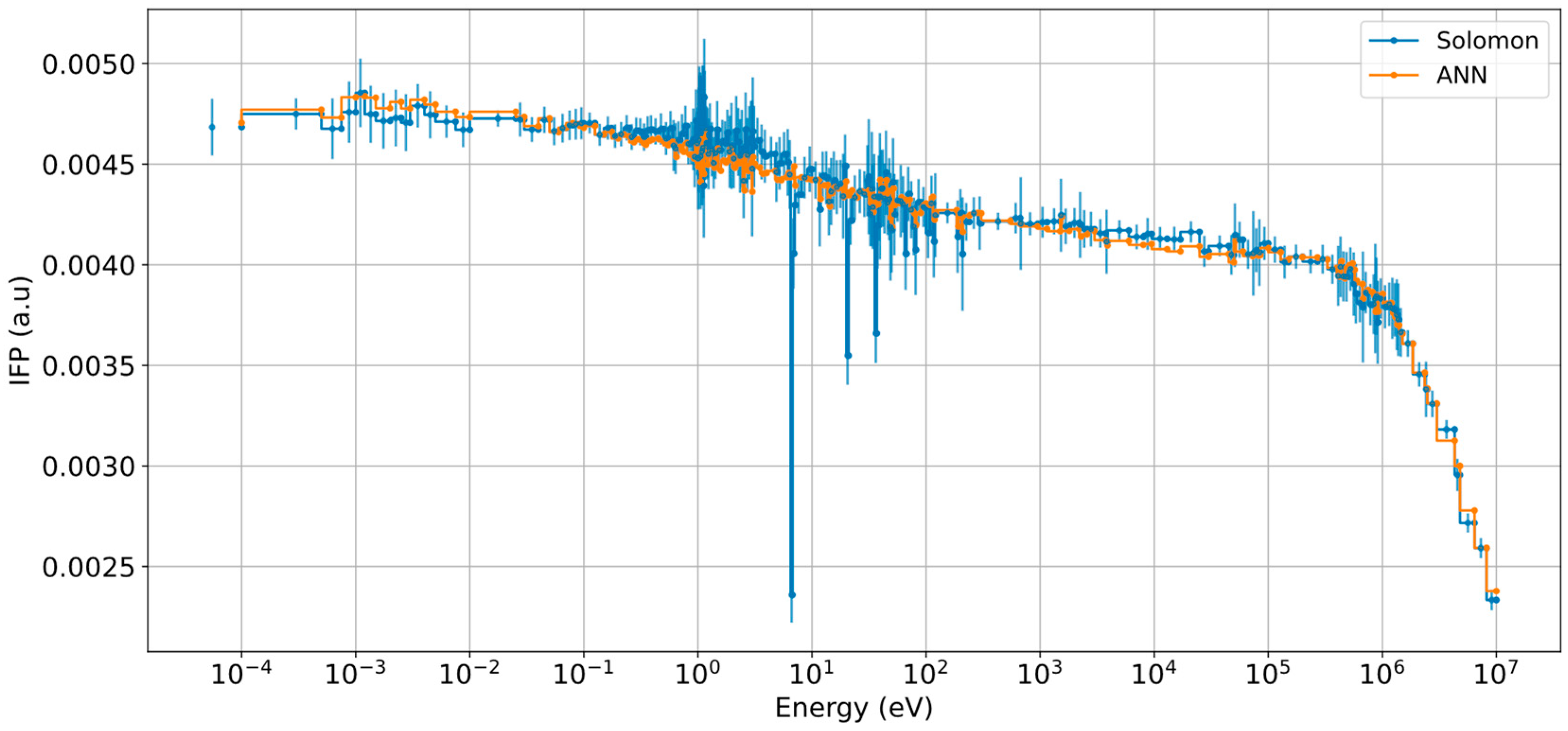
To further clarify the agreement or discrepancy between the IFP spectra by the Solomon solver and the selected ANN model, we use different energy structures varying from coarse to fine. In particular, we consider LANL-30g [34] and SCALE-238g [35] energy structures. The LANL-30g energy structure is relatively coarse and is mainly used for fusion applications; however, it has the same lethargy width in the resonance range. On the other hand, the SCALE-238g energy structure is used in various reactor physics applications. Figure 6 and Figure 7 show the comparison between the IFP spectra by the Solomon solver and the selected ANN model for the different energy structures.

To compare the group-wise IFP spectra quantitatively, we consider the average relative difference (Equation (6)) and the intersection (Equation (7)) via the Ruzicka similarity coefficient [36].

$$\overline{RD}=\frac{1}{G}{{\displaystyle \sum }}_{g=1}^G\frac{\left|R_g^{sol}-R_g^{ann}\right|}{max\left(R_g^{sol}, R_g^{ann}\right)},$$

(6)

$$S_{Ruz}=\frac{{{\displaystyle \sum }}_{g=1}^{G}min\left(R_g^{sol}, R_g^{ann}\right)}{{{\displaystyle \sum }}_{g=1}^{G}max\left(R_g^{sol}, R_g^{ann}\right)},$$

(7)

where $R_g^{sol}$ and $R_g^{ann}$ are the normalized mean IFPs in energy group $g$ by the Solomon solver and the ANN model, respectively. Note that the relative difference in Equation (6) is relative to the maximum of two distributions.

Table 4. Relative differences and Ruzicka similarity coefficient between normalized IFP spectra by Solomon solver and selected ANN model for different energy structures in Godiva core.

Energy Structure	$\overline{\mathit{R}\mathit{D}}$	$\mathbf{Maximum} \mathit{R}\mathit{D}$	${\mathit{S}}_{\mathit{R}\mathit{u}\mathit{z}}$
LANL-30g	1.8 × 10−2	7.0 × 10−2	0.98
SLAROM-UF-73g	2.7 × 10−2	1.81 × 10−1	0.97
SCALE-238g	7.1 × 10−2	6.46 × 10−1	0.93

lists the average and maximum relative differences and the Ruzicka similarity coefficients between the group-wise IFP spectra by the Solomon solver and the selected ANN model for each energy structure.

From Figure 5, Figure 6 and Figure 7 and Table 4, it can be observed that the agreement between the IFP distributions by the selected ANN model and the Solomon solver became worse as the energy structure became finer. The comparison indicates that the continuous IFP distribution by the selected ANN model is not the same as the true IFP distribution, but is a rough approximation of it. The discrepancy is particularly around the resonance energy range and a low energy range, as shown for the finer energy structure, which is closer to a continuous distribution, in Figure 7.

4.2.2. Simplified STACY Core

Similarly to the case of the Godiva core, ten ANN models constructed according to the widths and depths given in Table 2 have been trained on the training data. The training, validation, and test MSEs by each ANN model are given in

Table 5. Training results of ANN models on STACY data.

ANN Model	MSE
	Training	Validation	Test
ANN-1	3.78 × 10−1	3.81 × 10−1	3.83 × 10−1
ANN-2	3.78 × 10−1	3.79 × 10−1	3.81 × 10−1
ANN-3	3.77 × 10−1	3.78 × 10−1	3.80 × 10−1
ANN-4	3.77×10−1	3.78 × 10−1	3.80 × 10−1
ANN-5	3.97 × 10−1	4.00 × 10−1	4.02 × 10−1
ANN-6	3.78 × 10−1	3.78 × 10−1	3.80 × 10−1
ANN-7	3.78 × 10−1	3.78 × 10−1	3.80 × 10−1
ANN-8	3.83 × 10−1	3.83× 10−1	3.85 × 10−1
ANN-9	3.77 × 10−1	3.77 × 10−1	3.79 × 10−1
ANN-10	3.78 × 10−1	3.79 × 10−1	3.81 × 10−1

. It can be observed that the MSEs by the different ANN models did not show significant differences from each other; the maximum difference between the test MSE is about 5.6% between ANN-5 and ANN-9. According to the training result, ANN-9 is selected as it gives the marginally smaller test MSE. ANN-9 consists of 2148 parameters in total and 1920 of them are trainable. The training time for ANN-9 was about 12 min on a typical desktop computer with Intel(R) Core(TM) i7 (1.4 GHz) CPU and 32GB RAM.

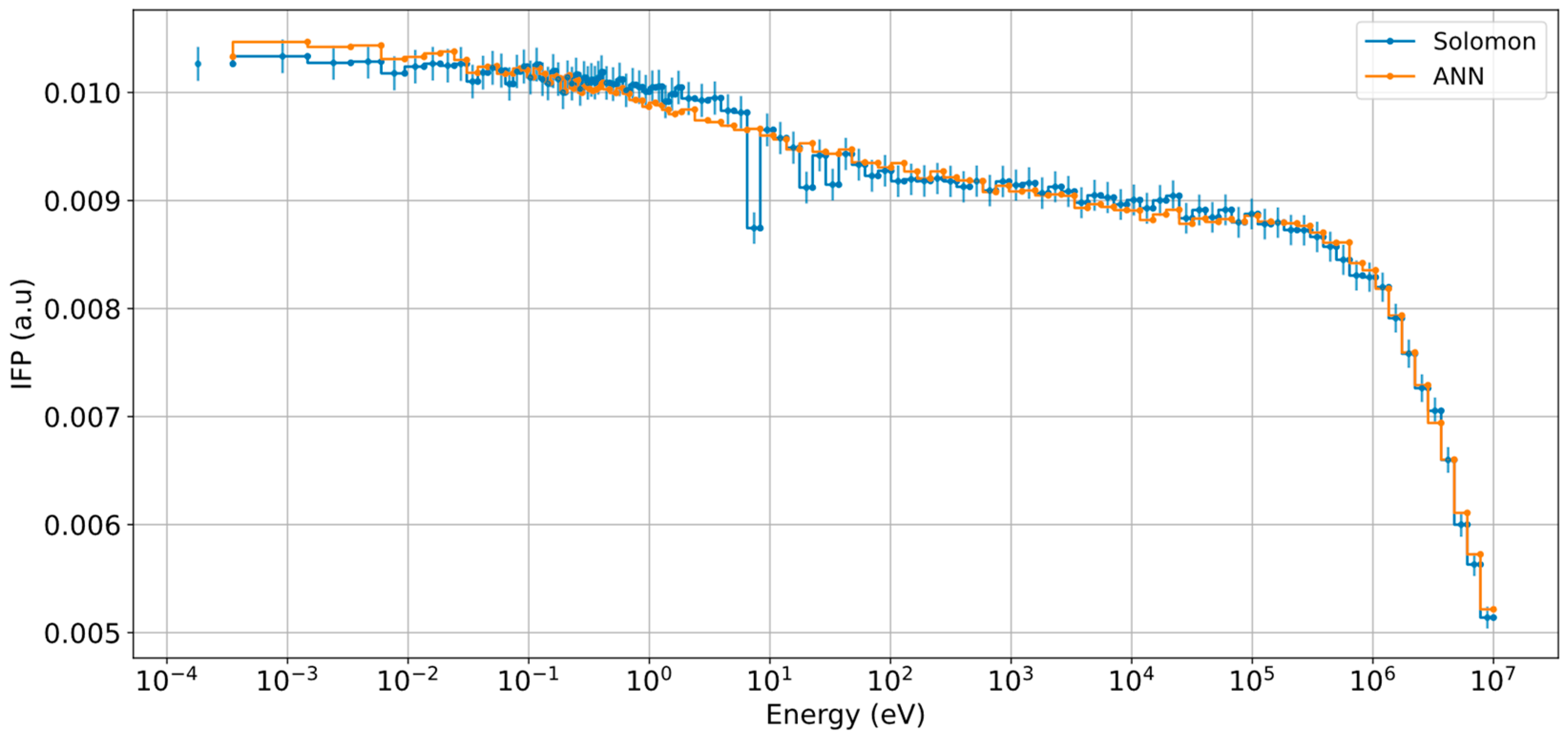
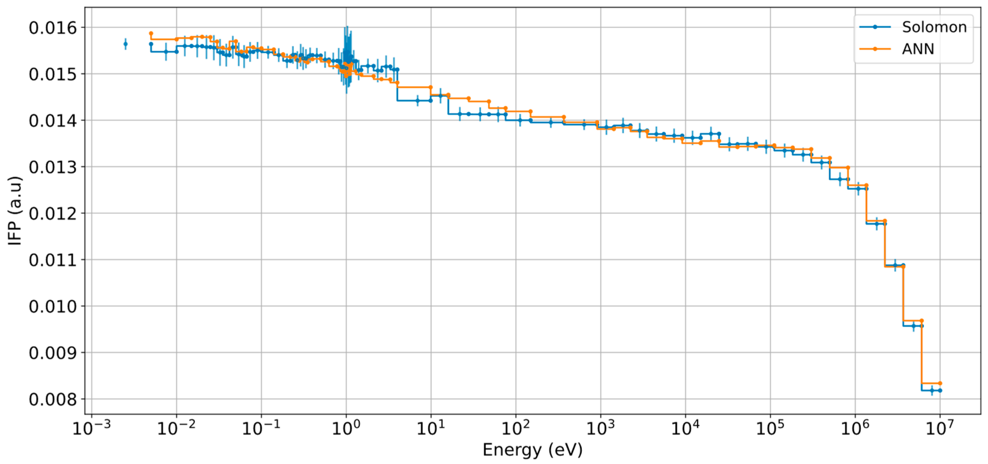
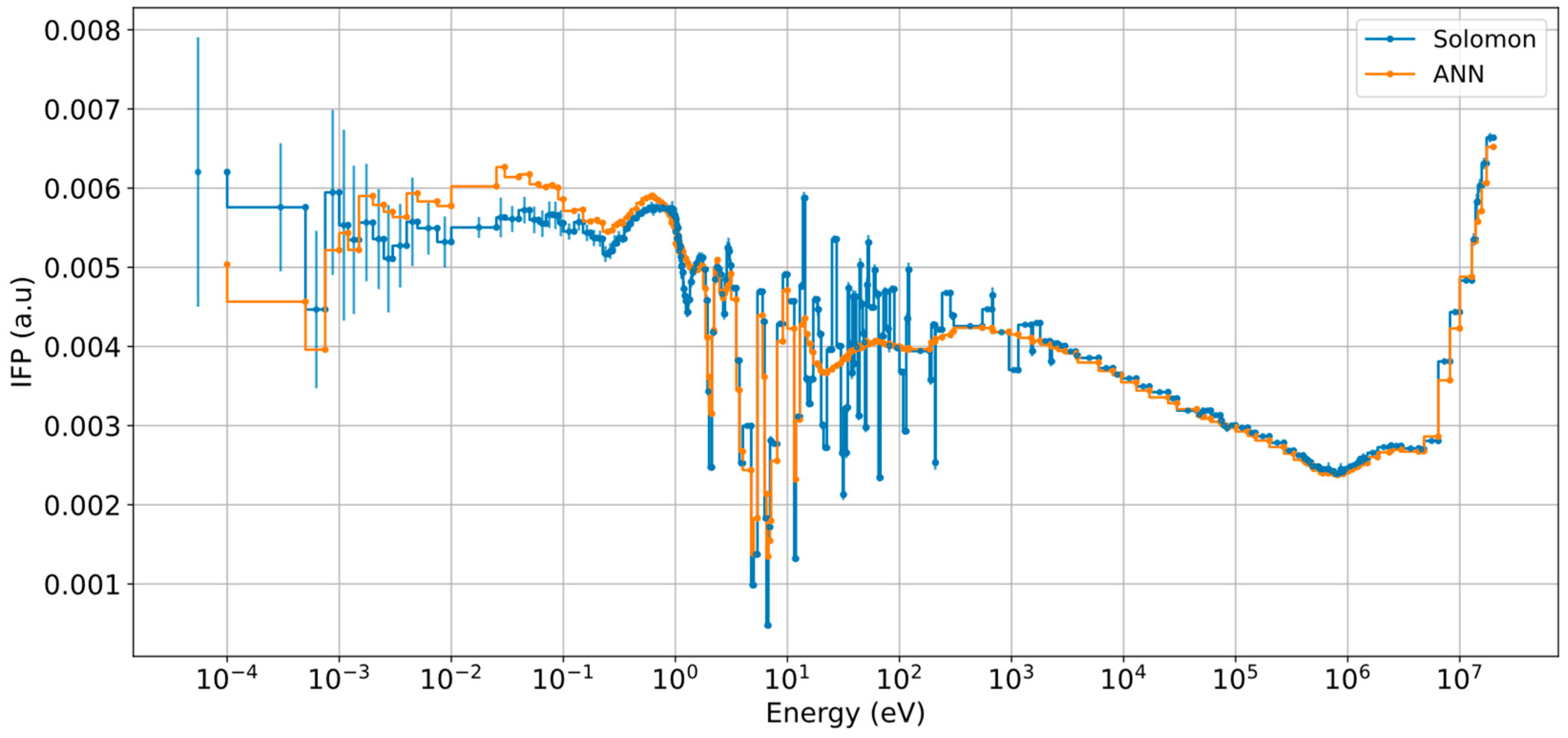
As done in the previous section, to compare the IFP distributions by the Solomon solver and the selected ANN model, we consider group-wise IFP spectra (see Equation (4)). The IFP spectra by the selected ANN model and Solomon solver are normalized to their respective integral values as described in Section 4.2.1. Figure 8 shows the comparison between the normalized IFP spectra by the Solomon solver and the selected ANN model using the SRAC-107g energy structure. It can be observed that the ANN model learned the general trend of the IFP distribution except for some discrepancies around the resonance energy range.

To further see the agreement or discrepancy between the IFP spectra by the Solomon solver and the selected ANN model, we used different energy structures varying from coarse to fine. The LANL-30g, WIMS-69g [37], and SCALE-238g energy structures are considered. Figure 9, Figure 10 and Figure 11 show the comparison between the normalized IFP spectra by the Solomon solver and the selected ANN model for each energy structure. It should be noted that the energy structures above 10 MeV in LANL-30g and SCALE-238g have been truncated because the IFP distribution up to 10 MeV was estimated by the ANN models in the simplified STACY core.

Table 6. Relative differences and Ruzicka similarity coefficient between normalized IFP spectra by Solomon solver and selected ANN model for different energy structures in simplified STACY core.

Energy Structure	$\overline{\mathit{R}\mathit{D}}$	$\mathbf{Maximum} \mathit{R}\mathit{D}$	${\mathit{S}}_{\mathit{R}\mathit{u}\mathit{z}}$
LANL-30g	8 × 10−3	1.7 × 10−2	0.99
WIMS-69g	9 × 10−3	2.3 × 10−2	0.99
SRAC-107g	9 × 10−3	9.5 × 10−2	0.99
SCALE-238g	1.5× 10−2	4.70 × 10−1	0.98

presents the quantitative comparison between the normalized IFP spectra by the Solomon solver and the selected ANN model in terms of the average relative difference and Ruzicka similarity coefficient (see Equations (6) and (7)).

The results shown in Figure 8, Figure 9, Figure 10 and Figure 11 and Table 6 indicate that the agreement between the IFP spectra by the Solomon solver and the selected ANN model increased as the energy structure became coarser. In the case of the finer energy structure of SCALE-238g, which is closer to continuous distribution compared to the other energy structures, the IFP spectrum by the selected ANN model shows increased discrepancies around the resonance energy range, indicating that the ANN model did not learn the resonance-like structure of the IFP distribution fully. Despite the discrepancies around the resonance energy region, the ANN model appeared to have learned the general trend of the IFP distribution in the simplified STACY core.

4.2.3. Comparison between ANN Model and Deterministic Neutron Transport Code PARTISN

To further analyze the estimated IFP distributions by the selected ANN models, we consider various two-dimensional comparisons between the IFP distributions by the selected ANN models and adjoint angular neutron flux distributions by the deterministic neutron transport code PARTISN [38].

To obtain adjoint angular neutron flux distributions in the fissile systems, adjoint eigenvalue calculations have been performed using the PARTISN code. For the Godiva core, the PARTISN calculation has been performed with 100 meshes (Δr = 0.087 cm) and Sn order of 180. The 73-group constants (e.g., cross-section) were obtained using the SLAROM-UF code [26] with a Legendre order of 5 using the JENDL-4.0 nuclear data library [39]. Due to the symmetry around the center of the core, a spherical geometry was used to produce adjoint angular neutron flux in the form ${\psi }^{*}\left(r,g,\mu \right)$, where $r$ is the radial variable, $g$ is the energy group, and $\mu$ is the angular cosine along the radial direction. In the case of the simplified STACY core, the PARTISN calculation has been done with 54 meshes (44 in the fuel region giving Δr = 0.5 cm and 10 in the reflector region giving Δr = 0.1 cm) and an Sn order of 16, which is the maximum. The 107-group constants were calculated by the MOSRA-SRAC code [40] via its PIJ routine using the JENDL-4.0 nuclear data library. Due to the XY symmetry around the center of the core, a cylindrical geometry was used to calculate the adjoint angular neutron flux in the form ${\psi }^{*}\left(r,g,\mu ,\eta \right)$, where $r$ is the radial variable in XY-plane, $g$ is the energy group, $\mu$ is the angular cosine along the radial direction, and $\eta$ is the angular cosine direction in the XY-plane perpendicular to the radial direction.

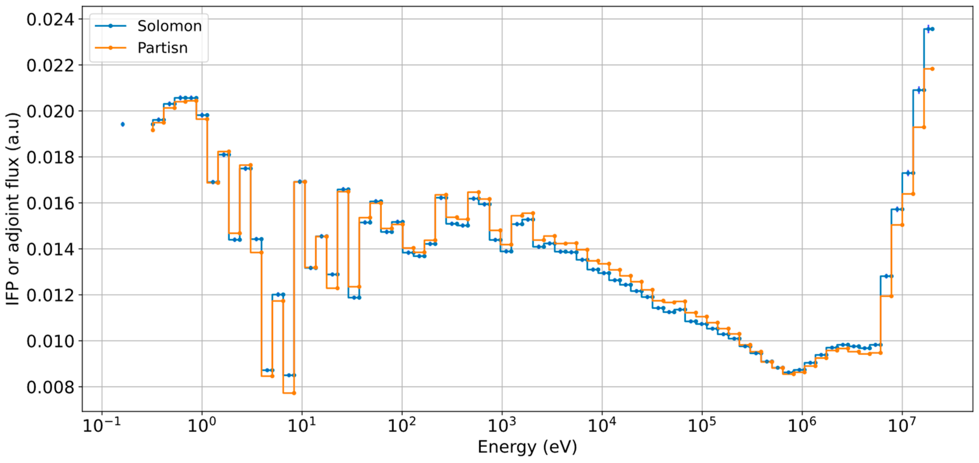
Before comparing the selected ANN models with the PARTISN code, we compare the group-wise IFP spectra by the Solomon solver and adjoint neutron flux spectra by the PARTISN code to confirm that the Monte Carlo and deterministic results are similar. Figure 12 and Figure 13 show the comparisons for the Godiva and simplified STACY cores, respectively. In both Godiva and simplified STACY cores, the IFP spectrum by the selected ANN model and adjoint neutron flux spectrum by the PARTISN code were normalized to their respective integral values. Despite the agreement on the general trend in the spectra, it can be seen that the comparisons show a slight discrepancy. However, the discrepancy possibly results from the uniform sampling distribution of energy in each group in calculating the IFP functions by the Solomon solver. In the case of the Godiva core, it was confirmed in the previous study [23] that the IFP spectrum and adjoint angular neutron flux spectrum are in agreement. On the other hand, the adjoint angular neutron flux spectra are calculated with group constants produced using an energy spectrum (typically a fission spectrum of ²³⁵U) as a weighting function in SLAROM-UF and MOSRA-SRAC codes.

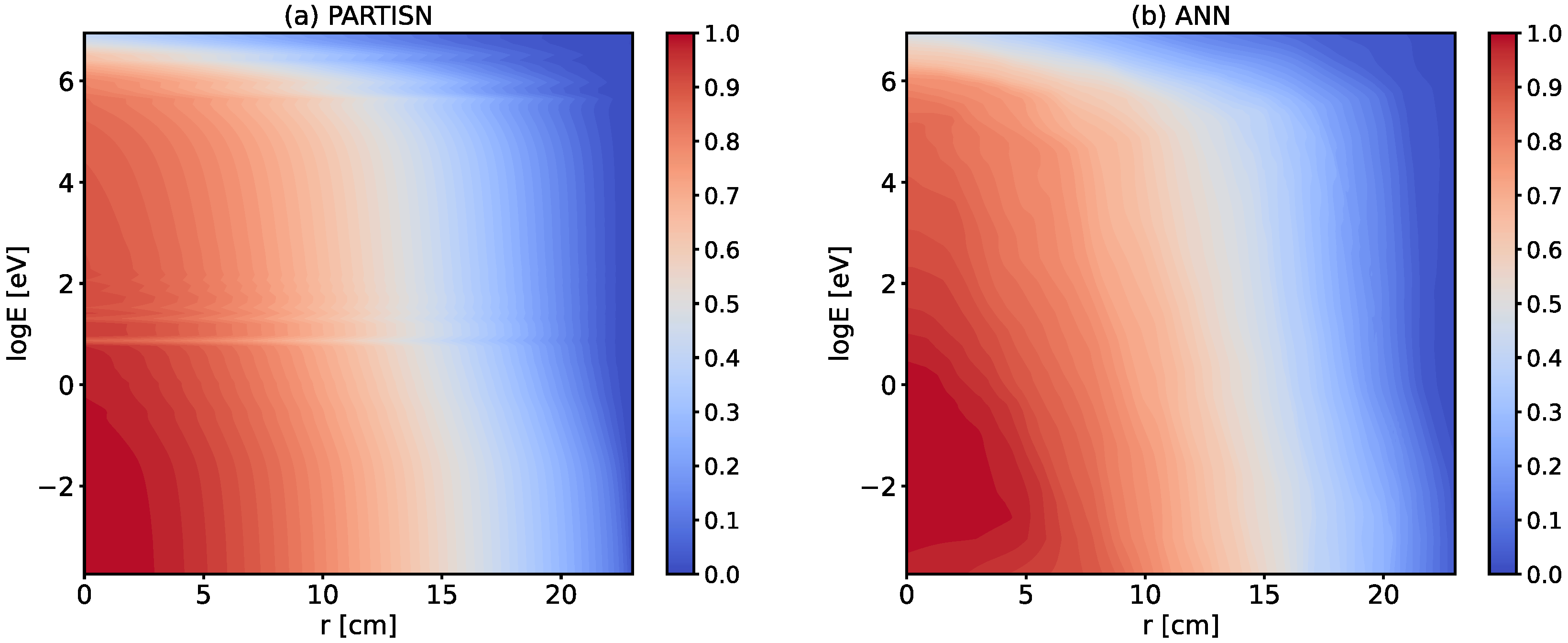
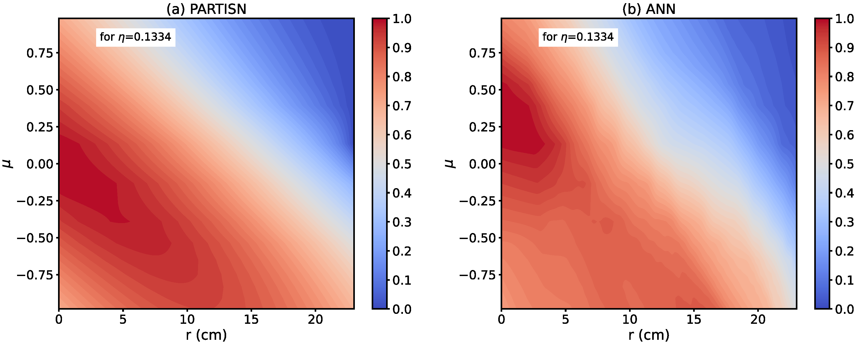
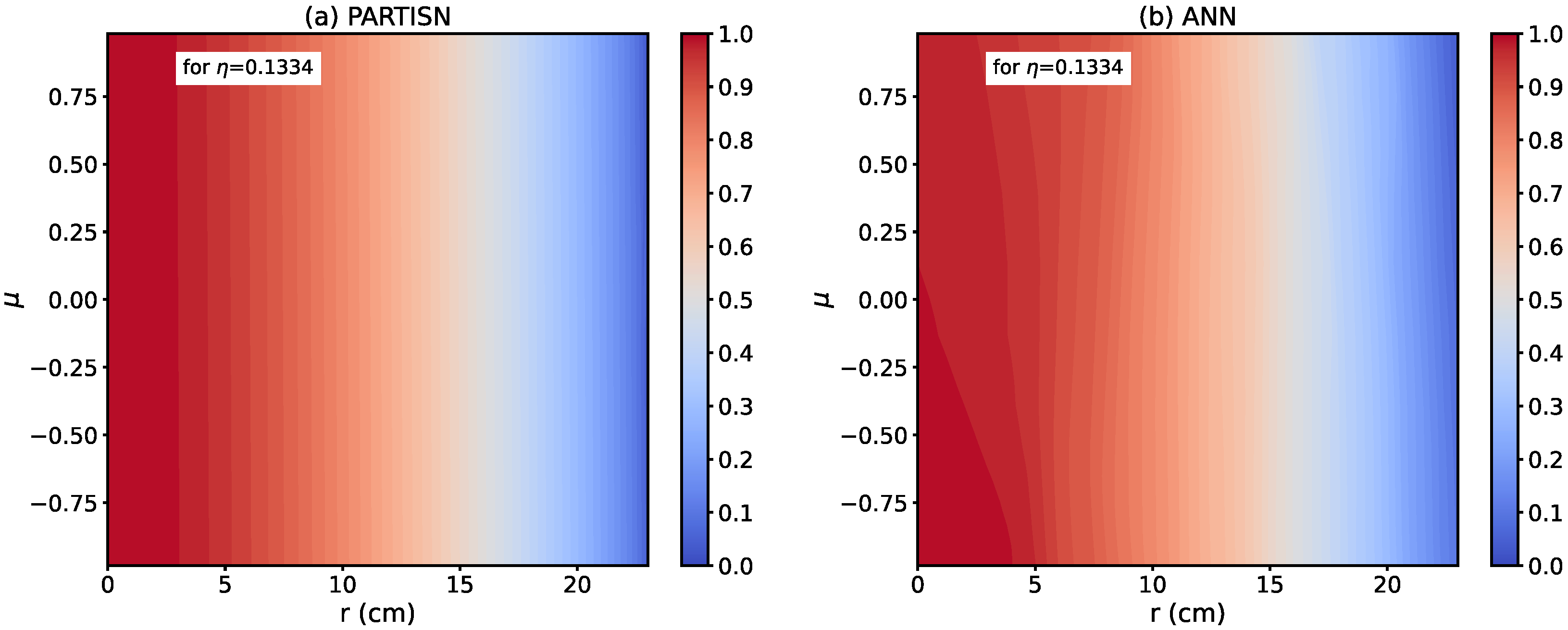
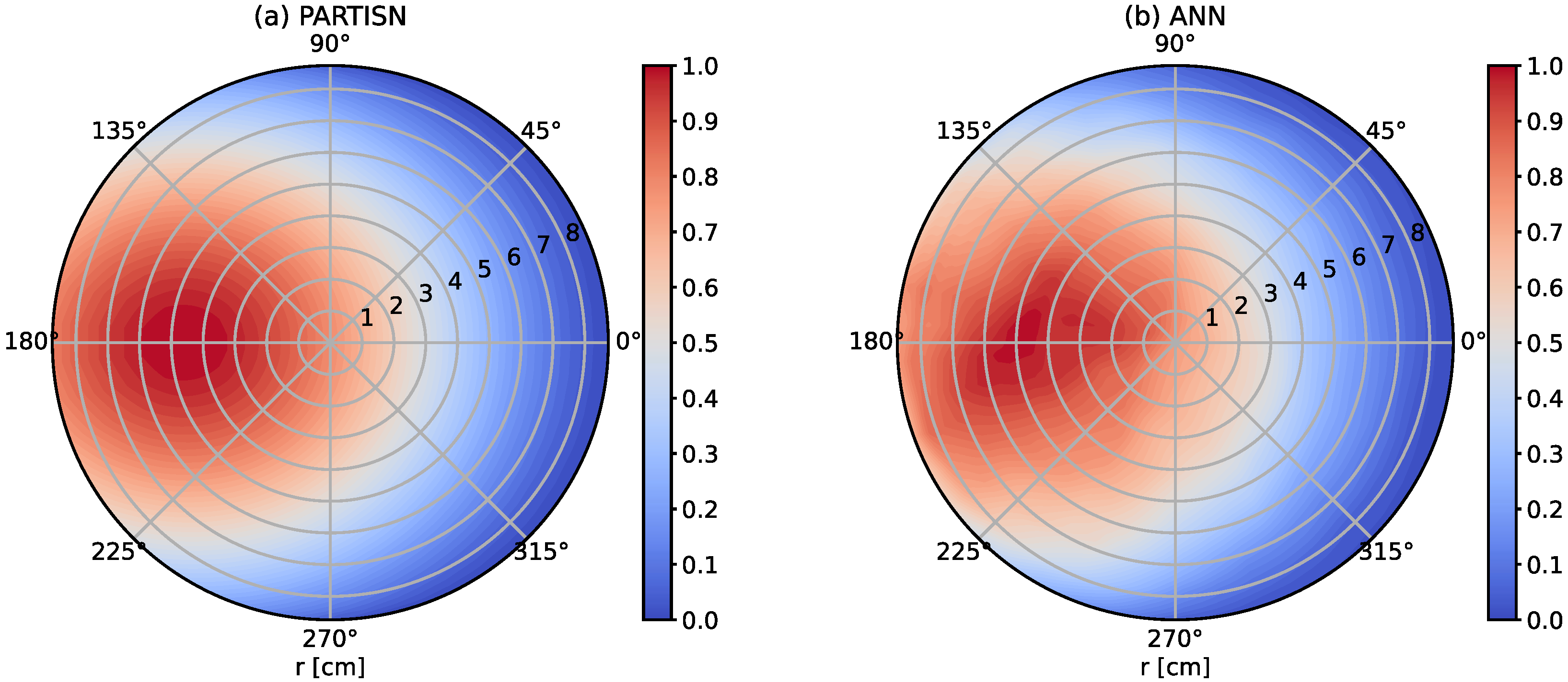
Since adjoint angular neutron fluxes by the PARTISN code were produced already in a group-wise manner, the IFP distributions in the given energy group by the ANN model were estimated by averaging IFPs at 20 equal intervals between the lower and upper energy boundary of the group to make the comparisons. Figure 14 and Figure 15 show the contour plots revealing the dependence of the IFP distributions and adjoint angular neutron flux distributions on energy and radial position for a given direction along the positive r in the figure. The average relative differences between the IFP distributions and adjoint angular neutron flux distributions were calculated using an expression similar to Equation (6) and are given in the captions of the figures.

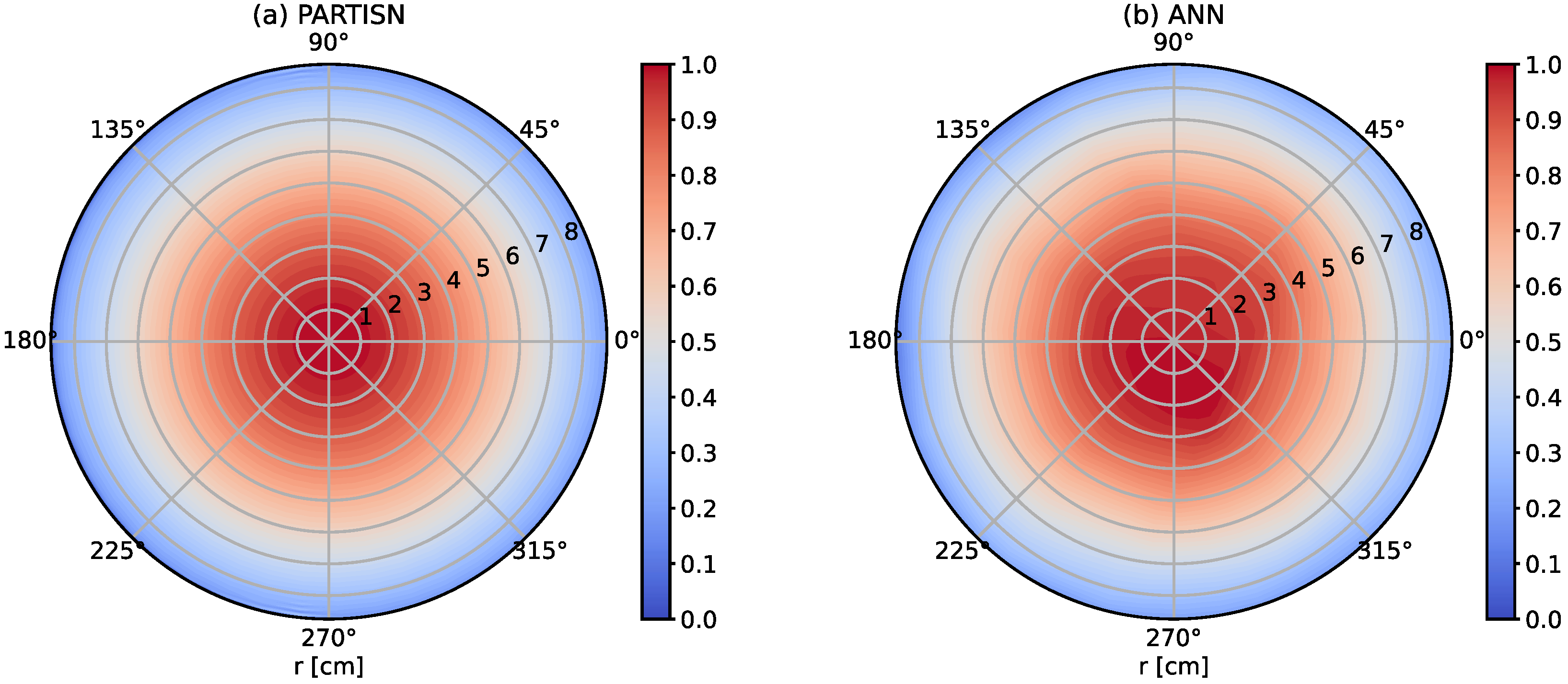
Figure 16, Figure 17, Figure 18 and Figure 19 present several representative two-dimensional plots showing the dependence of the IFP distribution by the selected ANN model and the adjoint angular neutron flux distribution by the PARTISN code on the radial and angular variables for given energy groups in both Godiva and simplified STACY cores. In the case of the Godiva core, the contour polar plots visualize the cross-sectional view of the adjoint angular neutron flux and IFP distributions for the given energy group and direction. It can be seen that the angular dependence of the adjoint angular neutron flux and IFP distribution decreases as the energy decreases. On the other hand, in the case of the simplified STACY core, the contour plots visualize the dependence of the adjoint angular neutron flux and IFP distributions on the radial and cosine angular variable $\mu$ for the given energy group and $\eta$ direction.

The comparisons shown in Figure 17 and Figure 19 appear similar, giving the average relative differences of 5.4 × 10⁻² and 2.8 × 10⁻², respectively. However, the IFP distribution by the selected ANN model shown in Figure 18 appears very irregular compared to its counterpart by the PARTISN code. In general, the comparisons show varying degrees of discrepancies between the adjoint angular neutron flux distributions by PARTISN and the IFP distributions by the selected ANN models.

Overall, the comparisons indicate that the estimated IFP distributions by the ANN models are only approximate representations of the true IFP distributions in both systems, suggesting that further improvements are necessary to increase the accuracy and applicability of the ANN model-based method. Despite the discrepancies, the obtained IFP distributions by the ANN models in this study suggest that the underlying IFP distributions in fissile systems may be estimated, albeit approximately, in a continuous manner via ANN model using data created from a Monte Carlo neutron transport calculation.

5. Conclusions

The method to estimate a continuous distribution of a quantity (e.g., neutron flux and reaction rate) in all phase-space variables using a fully connected feedforward artificial neural network (ANN) model with Monte Carlo-based training data has been proposed in this study. As a proof of concept of this method, the estimation of a continuous distribution of iterated fission probability (IFP), which is the quantity proportional to adjoint angular neutron flux, in all phase-space variables in a given fissile system has been performed in this work. To this end, two distinct fissile systems were considered: the fast spectrum Godiva core and the thermal spectrum simplified STACY core.

The ANN model was trained to learn the continuous distribution of IFP in each system from the Monte Carlo-based training data containing a discrete list of phase-space locations and corresponding IFP value pairs. The data were created by the IFP method implemented in the continuous-energy Monte Carlo neutron transport solver Solomon.

The estimated continuous IFP distributions by the ANN models were compared against the Monte Carlo-based data, which include the training data, by the Solomon solver in the form of the IFP spectrum. The comparison has been performed using three or four energy structures ranging from coarse to fine. The comparisons showed that across the energy structures, the average relative differences between the IFP spectra by the ANN models and Solomon solver were about 1.8–7.1% in the case of Godiva core and 0.8–1.5% in the case of the simplified STACY core. On the other hand, the maximum relative differences, which occurred around the resonance energy regions, were about 7.0–64.6% in the Godiva core and 1.7–47.0% in the simplified STACY core across the considered energy structures. The comparisons also showed that the discrepancy between the ANN models and Solomon solver increased as the energy structure became finer. Furthermore, the discrepancy is larger around the resonance energy regions, where the true IFP distributions showed peak-like structures while the estimated IFP distributions by the ANN models did not exhibit such structures fully. The comparisons indicated that the estimated IFP distributions by the ANN models were only approximate representations of the true IFP distributions in both systems.

The estimated continuous IFP distributions by the ANN models were further compared to the adjoint angular neutron flux distributions obtained with the deterministic neutron transport code PARTISN. To compare the ANN models and PARTISN, various two-dimensional distributions have been considered. The comparisons showed that the average relative differences between the estimated IFP distributions by the ANN models and the adjoint angular neutron flux distribution by the PARTISN code were about 2.8–11%. The comparisons revealed again that the estimated IFP distributions by the ANN models did not show resonance-energy-related peak structures fully, while the PARTISN results showed such structures.

Despite the varying discrepancies in the estimated IFP distributions by the ANN models when compared to the Monte Carlo neutron transport Solomon solver and deterministic neutron transport code PARTISN, this work showed that the underlying IFP distributions may be estimated, at least approximately, in a continuous manner via an ANN model from Monte Carlo-based training data. In the future, to make the ANN model-based method more applicable and to improve its accuracy, several important works need to be performed. First, an estimation of a continuous distribution of a forward angular or scalar neutron flux using the ANN model-based method from Monte Carlo-based data must be investigated. Second, alternative artificial neural network designs, cost functions, and different model and algorithmic hyperparameters should be considered to more accurately capture the finer details of IFP distributions such as resonance-energy related structures. Third, if the prior works prove to be good, then the ANN model-based method should be applied to more challenging problems in terms of geometry, material composition, and neutron flux or reaction rate distributions. Lastly, methods to quantify the uncertainty of the ANN model-based method need to be explored.

References

- Banerjee, K.; Martin, W.R. Kernel Density Estimation Method for Monte Carlo Global Flux Tallies. Nucl. Sci. Eng. 2012, 170, 234–250. [Google Scholar] [CrossRef]
- Burke, T.P.; Kiedrowski, B.C.; Martin, W.R. Kernel Density Estimation of Reaction Rates in Neutron Transport Simulations of Nuclear Reactors. Nucl. Sci. Eng. 2017, 188, 109–139. [Google Scholar] [CrossRef]
- Griesheimer, D.P. Functional Expansion Tallies for Monte Carlo Simulations. Ph.D. Thesis, The University of Michigan, Ann Arbor, MI, USA, 2005. [Google Scholar]
- Griesheimer, D.P.; Martin, W.R.; Holloway, J.P. Convergence Properties of Monte Carlo Functional Expansion Tallies. J. Comput. Phys. 2006, 211, 129–153. [Google Scholar] [CrossRef]
- Griesheimer, D.P.; Martin, W.R.; Holloway, J.P. Estimation of Flux Distributions with Monte Carlo Functional Expansion Tallies. Radiat. Prot. Dosim. 2005, 115, 428–432. [Google Scholar] [CrossRef]
- Ellis, M.; Gaston, D.; Forget, B.; Smith, K. Preliminary Coupling of the Monte Carlo Code OpenMC and the Multiphysics Object-Oriented Simulation Environment for Analyzing Doppler Feedback in Monte Carlo Simulations. Nucl. Sci. Eng. 2017, 185, 184–193. [Google Scholar] [CrossRef]
- Wendt, B.; Kerby, L.; Tumulak, A.; Leppänen, J. Advancement of Functional Expansion Capabilities: Implementation and Optimization in Serpent 2. Nucl. Eng. Des. 2018, 334, 138–153. [Google Scholar] [CrossRef]
- An, N.; Pan, Q.; Guo, X.; Huang, S.; Wang, K. A New Functional Expansion Tallies (FET) Method Based on Cutting Track-Length Estimation in RMC Code. Nucl. Eng. Des. 2022, 391, 111736. [Google Scholar] [CrossRef]
- Kiedrowski, B.C.; Brown, F.B.; Wilson, P.P.H. Adjoint-Weighted Tallies for k -Eigenvalue Calculations with Continuous-Energy Monte Carlo. Nucl. Sci. Eng. 2011, 168, 226–241. [Google Scholar] [CrossRef]
- Nauchi, Y.; Kameyama, T. Development of Calculation Technique for Iterated Fission Probability and Reactor Kinetic Parameters Using Continuous-Energy Monte Carlo Method. J. Nucl. Sci. Technol. 2010, 47, 977–990. [Google Scholar] [CrossRef]
- Ussachoff, L.N. Equation for the Importance of Neutrons, Reactor Kinetics and the Theory of Perturbations. In Proceedings of the International Conference on the Peaceful Uses of Atomic Energy, Geneva, Switzerland, 8–20 August 1955; pp. 503–510. [Google Scholar]
- Qiu, Y.; Wang, Z.; Li, K.; Yuan, Y.; Wang, K.; Fratoni, M. Calculation of Adjoint-Weighted Kinetic Parameters with the Reactor Monte Carlo Code RMC. Prog. Nucl. Energy 2017, 101, 424–434. [Google Scholar] [CrossRef]
- Shim, H.J.; Kim, C.H. Estimation of Adjoint-Weighted Kinetics Parameters in Monte Carlo Forward Calculations. In Proceedings of the PHYSOR 2010: Advances in Reactor Physics to Power the Nuclear Renaissance, Pittsburgh, PA, USA, 9–14 May 2010; American Nuclear Society: Pittsburgh, PA, USA, 2010. [Google Scholar]
- Shim, H.J.; Kim, C.H. Monte Carlo Fuel Temperature Coefficient Estimation by an Adjoint-Weighted Correlated Sampling Method. Nucl. Sci. Eng. 2014, 177, 184–192. [Google Scholar] [CrossRef]
- Shim, H.J.; Kim, C.H. Adjoint Sensitivity and Uncertainty Analyses in Monte Carlo Forward Calculations. J. Nucl. Sci. Technol. 2011, 48, 1453–1461. [Google Scholar] [CrossRef]
- Chiba, G.; Nagaya, Y.; Mori, T. On Effective Delayed Neutron Fraction Calculations with Iterated Fission Probability. J. Nucl. Sci. Technol. 2011, 48, 1163–1169. [Google Scholar] [CrossRef]
- Kiedrowski, B.C.; Brown, F.B. Adjoint-Based k-Eigenvalue Sensitivity Coefficients to Nuclear Data Using Continuous-Energy Monte Carlo. Nucl. Sci. Eng. 2013, 174, 227–244. [Google Scholar] [CrossRef]
- Perfetti, C.M.; Rearden, B.T.; Martin, W.R. SCALE Continuous-Energy Eigenvalue Sensitivity Coefficient Calculations. Nucl. Sci. Eng. 2016, 182, 332–353. [Google Scholar] [CrossRef]
- Terranova, N.; Mancusi, D.; Zoia, A. New Perturbation and Sensitivity Capabilities in Tripoli-4®. Ann. Nucl. Energy 2018, 121, 335–349. [Google Scholar] [CrossRef]
- Truchet, G.; Leconte, P.; Palau, J.M.; Archier, P.; Tommasi, J.; Santamarina, A.; Peneliau, Y.; Zoia, A.; Brun, E. Sodium Void Reactivity Effect Analysis Using the Newly Developed Exact Perturbation Theory in Monte-Carlo Code TRIPOLI-4. In Proceedings of the PHYSOR 2014: The Role of Reactor Physics toward a Sustainable Future, Kyoto, Japan, 28 September–3 October 2014. [Google Scholar]
- Truchet, G.; Leconte, P.; Santamarina, A.; Brun, E.; Damian, F.; Zoia, A. Computing Adjoint-Weighted Kinetics Parameters in Tripoli-4® by the Iterated Fission Probability Method. Ann. Nucl. Energy 2015, 85, 17–26. [Google Scholar] [CrossRef]
- Terranova, N.; Truchet, G.; Zmijarevic, I.; Zoia, A. Adjoint Neutron Flux Calculations with Tripoli-4®: Verification and Comparison to Deterministic Codes. Ann. Nucl. Energy 2018, 114, 136–148. [Google Scholar] [CrossRef]
- Tuya, D.; Nagaya, Y. Approximate Estimation of Iterated Fission Probability by Deep Neural Network. In Proceedings of the International Conference on Nuclear Engineering (ICONE-30), Kyoto, Japan, 21–26 May 2023; American Society of Mechanical Engineers: Kyoto, Japan, 2023. [Google Scholar]
- Nagaya, Y.; Ueki, T.; Tonoike, K. Solomon: A Monte Carlo Solver for Criticality Safety Analysis. In Proceedings of the 11th International Conference on Nuclear Criticality Safety, Paris, France, 15–20 September 2019. [Google Scholar]
- LaBauve, R.J. Bare, Highly Enriched Uranium Sphere (Godiva). In International Handbook of Evaluated Criticality Safety Benchmark Experiments; Nuclear Energy Agency; OECD: Paris, France, 2003. [Google Scholar]
- Hazama, T.; Chiba, G.; Sugino, K. Development of a Fine and Ultra-Fine Group Cell Calculation Code SLAROM-UF for Fast Reactor Analyses. J. Nucl. Sci. Technol. 2006, 43, 908–918. [Google Scholar] [CrossRef]
- Nagaya, Y.; Mori, T. Impact of Perturbed Fission Source on the Effective Multiplication Factor in Monte Carlo Perturbation Calculations. J. Nucl. Sci. Technol. 2005, 42, 428–441. [Google Scholar] [CrossRef]
- Okumura, K.; Kugo, T.; Kaneko, K.; Tsuchihashi, K. SRAC2006: A Comprehensive Neutronics Calculation Code System; JAEA-Data/Code 2007-004; Japan Atomic Energy Agency: Tōkai, Japan, 2007.
- Goodfellow, I.; Bengio, Y.; Courville, A. Deep Learning; MIT Press: Cambridge, MA, USA, 2016. [Google Scholar]
- Goodfellow, I.; Bengio, Y.; Courville, A. Practical Methodology. In Deep Learning; MIT Press: Cambridge, MA, USA, 2016; pp. 416–437. [Google Scholar]
- Kingma, D.P.; Ba, J. Adam: A Method for Stochastic Optimization. arXiv 2014, arXiv:1412.6980. [Google Scholar]
- Prechelt, L. Early Stopping—But When? Neural Networks: Tricks of the Trade; Springer: Berlin/Heidelberg, Germany, 1998; pp. 55–69. [Google Scholar]
- Yeo, I.K.; Johnson, R.A. A New Family of Power Transformations to Improve Normality or Symmetry. Biometrika 2000, 87, 954–959. [Google Scholar] [CrossRef]
- MacFarlane, R.E.; Douglas, W.M. The NJOY Nuclear Data Processing System, Version 91 (LA-12740-M); Los Alamos National Laboratory: Los Alamos, NM, USA, 1994.
- Rearden, B.T.; Jessee, M.A. SCALE Code System (ORNL/TM-2005/39); Oak Ridge National Lab. (ORNL): Oak Ridge, TN, USA, 2018.
- Cha, S.H. Comprehensive Survey on Distance/Similarity Measures between Probability Density Functions. Int. J. Math. Models Methods Appl. Sci. 2007, 1, 300–307. [Google Scholar]
- Lindley, B.A.; Hosking, J.G.; Smith, P.J.; Powney, D.J.; Tollit, B.S.; Newton, T.D.; Perry, R.; Ware, T.C.; Smith, P.N. Current Status of the Reactor Physics Code WIMS and Recent Developments. Ann. Nucl. Energy 2017, 102, 148–157. [Google Scholar] [CrossRef]
- Alcouffe, R.E.; Baker, R.S.; Dahl, J.A.; Turner, S.A.; Ward, R.C. PARTISN: A Time-Dependent, Parallel Neutral Particle Transport Code System, LA-UR-08-07258; Los Alamos National Laboratory: Los Alamos, NM, USA, 2008.
- Shibata, K.; Iwamoto, O.; Nakagawa, T.; Iwamoto, N.; Ichihara, A.; Kunieda, S.; Chiba, S.; Furutaka, K.; Otuka, N.; Ohasawa, T.; et al. JENDL-4.0: A New Library for Nuclear Science and Engineering. J. Nucl. Sci. Technol. 2011, 48, 1–30. [Google Scholar] [CrossRef]
- Okumura, K. MOSRA-SRAC: Lattice Calculation Module of the Modular Code System for Nuclear Reactor Analyses MOSRA, JAEA-Data/Code 2015-015; Japan Atomic Energy Agency: Tōkai, Japan, 2015.
Figure 1.
Monte Carlo method for estimating IFP at phase-space location .
Figure 2.
Energy structure for energy sampling.
Figure 3.
Monte Carlo-based data creation procedure.
Figure 4.
Fully connected feedforward ANN.
Figure 5.
Group-wise normalized IFP spectra by Solomon solver and ANN model in Godiva core with SLAROM-UF-73g energy structure (3 is given for Solomon).
Figure 6.
Group-wise normalized IFP spectra by Solomon solver and selected ANN model in Godiva core on LANL-30g energy structure (3 is given for Solomon).
Figure 7.
Group-wise normalized IFP spectra by Solomon solver and selected ANN model in Godiva core on SCALE-238g energy structure (3 is given for Solomon).
Figure 8.
Group-wise normalized IFP spectra by Solomon solver and selected ANN model in simplified STACY core on SRAC-107g energy structure (3 is given for Solomon).
Figure 9.
Group-wise normalized IFP spectra by Solomon solver and selected ANN model in simplified STACY core on LANL-30g energy structure (3 is given for Solomon).
Figure 10.
Group-wise normalized IFP spectra by Solomon solver and selected ANN model in simplified STACY core on WIMS-69g energy structure (3 is given for Solomon).
Figure 11.
Group-wise normalized IFP spectra by Solomon solver and selected ANN model in simplified STACY core on SCALE-238g energy structure (3 is given for Solomon).
Figure 12.
IFP spectrum by Solomon solver and adjoint neutron flux spectrum by PARTISN in Godiva core (normalized).
Figure 13.
IFP spectrum by Solomon solver and adjoint neutron flux spectrum by PARTISN in simplified STACY core (normalized).
Figure 14.
Contour plot of normalized adjoint angular neutron flux by PARTISN and normalized IFP by selected ANN model (for i.e., the direction is along r) in Godiva core, = 7 × 10⁻².
Figure 15.
Contour plot of normalized adjoint angular neutron flux by PARTISN and normalized IFP by selected ANN model (for = 0.982, = 0.133) in simplified STACY core, = 7.1 × 10⁻².
Figure 16.
polar contour plot of normalized adjoint angular neutron flux distribution by PARTISN and normalized IFP distribution by ANN model in Godiva core (for the highest energy group and direction in 0° in the figure), = 4.4 × 10⁻².
Figure 17.
polar contour plot of normalized adjoint angular neutron flux distribution by PARTISN and normalized IFP distribution by ANN model in Godiva core (for the lowest energy group and direction in 180° in the figure), = 5.4 × 10⁻².
Figure 18.
contour plot of normalized adjoint angular neutron flux distribution by PARTISN and normalized IFP distribution by ANN model in simplified STACY core (for the highest energy group), = 1.1 × 10⁻¹.
Figure 19.
contour plot of normalized adjoint angular neutron flux distribution by PARTISN and normalized IFP distribution by ANN model in simplified STACY core (for the lowest energy group), = 2.8 × 10⁻².