CFD Simulations of Hydrogen Tank Fuelling: Sensitivity to Turbulence Model and Grid Resolution

Abstract

CFD modelling of compressed hydrogen fuelling provides information on the hydrogen and tank structure temperature dynamics required for onboard storage tank design and fuelling protocol development. This study compares five turbulence models to develop a strategy for cost-effective CFD simulations of hydrogen fuelling while maintaining a simulation accuracy acceptable for engineering analysis: RANS models k-ε and RSM; hybrid models SAS and DES; and LES model. Simulations were validated against the fuelling experiment of a Type IV 29 L tank available in the literature. For RANS with wall functions and blended models with near-wall treatment, the simulated average hydrogen temperatures deviated from the experiment by 1–3% with CFL ≈ 1–3 and dimensionless wall distance y⁺ ≈ 50–500 in the tank. To provide a similar simulation accuracy, the LES modelling approach with near-wall treatment requires mesh with wall distance y⁺ ≈ 2–10 and demonstrates the best-resolved flow field with larger velocity and temperature gradients. LES simulation on this mesh, however, implies a ca. 60 times longer CPU time compared to the RANS modelling approach and 9 times longer compared to the hybrid models due to the time step limit enforced by the CFL ≈ 1.0 criteria. In all cases, the simulated pressure histories and inlet mass flow rates have a difference within 1% while the average heat fluxes and maximum hydrogen temperature show a difference within 10%. Compared to LES, the k-ε model tends to underestimate and DES tends to overestimate the temperature gradient inside the tank. The results of RSM and SAS are close to those of LES albeit of 8–9 times faster simulations.

1. Introduction

The increasing availability of computational resources and the progress in numerical algorithms prompt the use of numerical modelling approaches, e.g., Computational Fluid Dynamics (CFD), for the design of safety-critical hydrogen applications. This is particularly applicable to the safety of compressed gaseous hydrogen storage systems, including the design of hydrogen fuelling protocols. CFD is particularly attractive as a non-destructive method of research in the safety of high-pressure hydrogen storage as experimental studies may be expensive due to potential tank ruptures. There is, however, a lack of clarity regarding the efficiency of modelling strategies and practices. This paper aims to systematically and coherently examine the effect of the turbulence model and numerical grid choice on the simulation results of compressed hydrogen fuelling from the perspective of the accuracy and computational costs expected in practical engineering.

For hydrogen storage and transportation, high-pressure gaseous hydrogen storage tanks currently represent the most developed technology due to their technical reliability, acceptable efficiency, and affordability [1]. Concerning the hydrogen fuelling of such tanks, it is recommended that the duration of the fuelling is of the order of 3–5 min [2]. Gas compression and stratification during the fuelling typically lead to elevated temperatures and temperature non-uniformities (hot spots) inside a storage tank. The increase in the gas temperature can affect the state of charge (SoC) of the tank, which is dependent on the hydrogen density at the current pressure and temperature. Most importantly, the higher temperature can affect the performance of the tank materials due to the heat transfer combined with thermal stress [3]. Hydrogen temperature non-uniformity can be especially pronounced in tanks with comparatively large length-over-diameter ratios, L/D [4]. For fast fuelling, locally elevated temperatures can increase the temperatures of the liner and the composite overwrap, which, with time, may compromise the mechanical performance of the composite due to numerous refuelling [5]. For this reason, the United Nations Global Technical Regulation No. 13 (GTR#13) and other documents, e.g., SAE J2601, require that the hydrogen temperature in the tank should be limited between −40 °C and +85 °C [6,7], which should be addressed in a fuelling protocol.

Experiments, reduced models [8], and numerical simulations have been used to understand and control the maximum regulated temperature in the tank during fuelling. Reduced models can calculate only the average (bulk) hydrogen temperatures in tanks as they are based on the mass and energy conservation equations combined with the empirical heat transfer correlations, etc. They are not able to assess the hydrogen temperature non-uniformity. The experimental measurements of temperature distribution inside the tank in various locations would be the most trustworthy yet expensive assessment way for tank fuelling. Unfortunately, the spatial resolution of temperature distribution is limited by the number of probes, and the influence of the probe setup on the fuelling is not well known. The use of CFD for three-dimensional (3D) numerical simulations offers insights into the pressure, temperature, flow velocity fields in the tank, and any physical parameters of interest that allow for the design and optimisation of the fuelling process. However, the CFD results depend significantly on the applied models, where the choice of turbulence models, the equation of state, and grid design are especially important.

Various Reynolds-averaged-based turbulence models have been applied in fuelling simulations. Early simulations were conducted by Dicken and Mérida [9] in 2007. The authors conducted a 2D simulation with a standard k-ε model and a modified turbulence production term coefficient in the dissipation equation, C_ε1. The value of C_ε1 was changed from 1.44 to 1.52 to avoid overpredicting the entrainment rate in jets [10]. For convenience, hereafter, it will be referred to as the modified k-ε model. The modified k-ε model was later widely used by other authors, for example, in studies [11,12,13,14,15]. Another popular turbulence model for fuelling simulations is the k-ω Shear Stress Transport (SST) model [16]. It combines the robustness of the k-ω turbulence model in the near-wall regions with the capabilities of the k-ε model in regions distant from the boundary walls. The k-ω SST turbulence model has been used by Heitsch et al. [17] in 2011, Suryan et al. [18] in 2012, Melideo [19] in 2019, and Remi et al. [4] in 2022. The use of other turbulence models for hydrogen fuelling simulations is reviewed and summarised by Bourgeois et al. [20]: Spalart and Allmaras [21], standard k-ε [22], high Reynolds number k-ε [23], realisable k-ε [24], RNG k-ε [25,26], and Reynolds Stress Model (RSM) [27]. The authors [20] indicate that more advanced turbulence models (e.g., Scale-Adaptive Simulation (SAS) [28] or even LES when possible) may be used to improve the accuracy of the results in the case of complex flow regimes like transitional flows and stratified temperature fields.

However, only a few comparative studies have been conducted so far, making turbulence model selection for the fuelling simulations not obvious. In 2013, Suryan et al. [29] applied four turbulence models (realisable k-ε, RNG k-ε model, RSM, k-ω SST) in 2D CFD simulations of hydrogen fuelling, implementing an axial symmetry approach. The authors concluded that the realisable k-ε and the RSM are the most suitable models; however, the simulation results with the four turbulent models were similar and the advantage of RSM stated by the authors was not obvious. In 2014, Galassi et al. [12] concluded that the difference between the modified k-ε and SST model is about 10% in the calculated temperature profiles, but no details were provided. In 2023, Martin et al. [30] tested different models (k-ε, k-ω SST, SAS, and RSM) and concluded that the RSM model was the best to represent the behaviour of the cold jet affecting the internal tank walls and to reproduce thermal stratifications inside the tank during the fuelling. The experimentally measured hydrogen temperatures in two thermocouples (TCs) inside the tank at 3000 s were 49 °C and 26 °C, while the simulations using the RSM model resulted in values of 46 °C and 29 °C, respectively, underestimating the temperature gradient by 26%. The results obtained with the use of the SAS model gave 44 °C and 31 °C, underestimating the temperature gradient by 43%. In the same study [30], the results obtained with the use of the k-ω SST model provided simulated temperatures of 40 °C and 35 °C, respectively, underestimating the temperature gradient by 78%. This led the authors to the conclusion that the model is “disqualified” for refuelling simulations. At the same time, in 2023, Gonin et al. carried out similar experiments and simulations with a 36 L tank [31]. The authors significantly improved the thermal gradient prediction using the k-ω SST Scale-Adaptive Simulation (SAS) model (98 °C, 49 °C) compared to the experimental data (99 °C, 48 °C) measured by 10 TCs, underestimating the temperature gradient by only 4%. Indeed, the “conventional” k-ω SST model in their simulations seriously underestimated the difference between the maximum and minimum temperatures (83 °C, 57 °C) by 47%. The authors claimed that the k-ω SST SAS turbulence model reduces the overprediction of the turbulence level and the associated thermal diffusion. However, the authors did not give a detailed comparison between the different models, which remains a knowledge gap.

Only a few studies on fuelling investigated grid sensitivity. A full grid sensitivity analysis can be challenging due to the prohibitively long computational time. As mentioned by Galassi et al. [12], a typical hydrogen fuelling simulation with hundreds of thousands of control volumes (CVs) may take weeks or months to complete. In 2014, Galassi et al. [12] tested four different grids with different local refinements in areas of pipe and near the boundary between solid and gas media. The difference in the calculated maximum temperatures was claimed to be small with deviations from the experimental values within 7%. In 2017, Melideo et al. [32] showed that there is no difference in adding a boundary-layer mesh near the gas–solid boundary. However, those conclusions are limited to the modified k-ε model with wall functions. Therefore, a comprehensive grid sensitivity study for fuelling remains not well investigated.

As summarised above, the impacts of the turbulence model choice and numerical grid design have not been systematically studied in terms of the computational costs versus prediction accuracy. The disparity between the characteristic time and length scales present in the problem of transient real gas flow during hydrogen fuelling may require significant computational resources for 3D simulations. CFD simulations with numerical grids over millions of control volumes requiring months to finish one simulation are available in the literature. This study aims to reduce the computational cost of compressible hydrogen fuelling simulations while maintaining a reasonable simulation accuracy. The sensitivity of hydrogen fuelling 3D CFD simulations to the turbulence model choice and numerical grid resolution will be studied. For the first time, both RANS (Reynolds-averaged Navier–Stokes equations) models (modified k-ε, RSM) and three non-RANS models (namely LES, SAS, and DES) are applied to simulate hydrogen fuelling and compared in terms of the accuracy and computational cost. The experimental hydrogen temperature dynamics are used to validate the simulations and as a basis for comparison of the models’ accuracy.

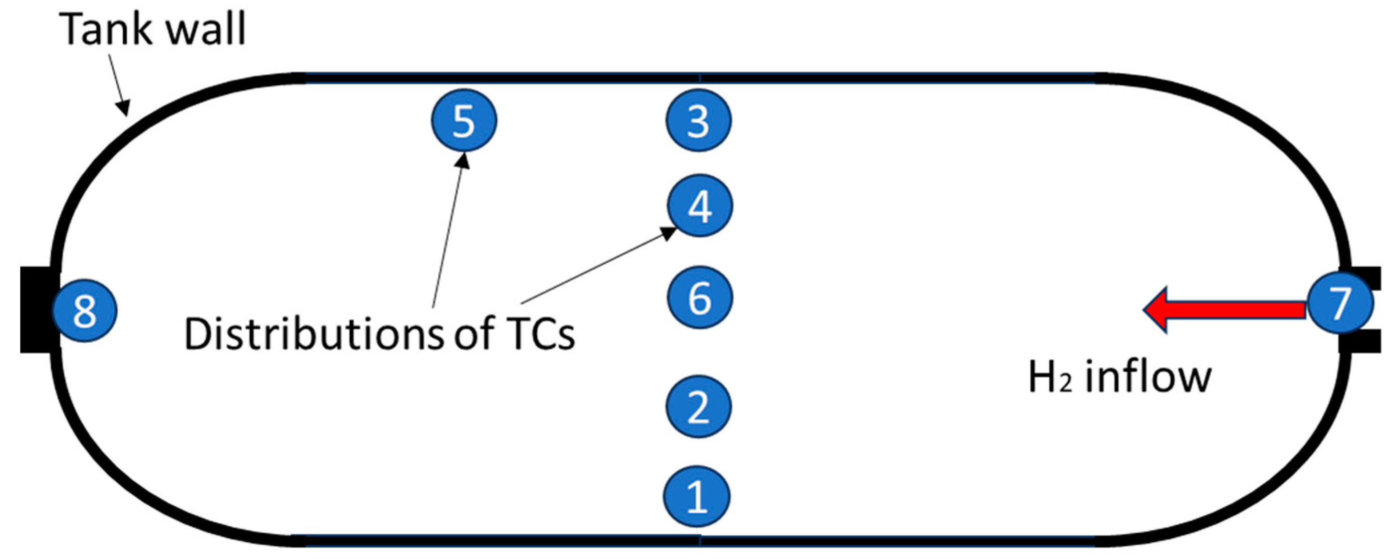
2. Validation Experiment

A series of experiments and CFD simulations on fuelling were performed by the research group at the Joint Research Centre (JRC) of the European Commission. One of the JRC experiments was well described in 2016 [13] and is chosen here for the comparison of the different turbulence models’ performance. The hydrogen temperature history has been well reproduced by the authors in the original publication [13] with the modified standard k-ε model.

The test cylinder used in the experiment was a 29 L Type IV tank. The fuelling started from 2 MPa and finished at 77 MPa. The geometry and properties of the tank materials are described in

Table 1. Parameters of the experimental Type IV tank [13] used for fuelling simulations.

Overall Tank Characteristics
Volume (L)	29
External length (mm)	827
External diameter (mm)	279
Inlet diameter (mm)	3
Thickness of liner (mm)	2.7
Thickness of composite shell (mm)	21.8
High-Density Polyethylene (HDPE) Liner Properties
Density (kg/m3)	945
Thermal conductivity (W/m/K)	0.385
Specific heat capacity (J/kg/K)	1580
Carbon Fibre Reinforced Polymer (CFRP) Overwrap Properties
Density (kg/m3)	1494
Thermal conductivity (W/m/K)	0.74
Specific heat capacity (J/kg/K)	1120

.

Figure 1 shows the positioning of eight TCs inside the tank. The diameter of all TCs is 1 mm, they all are of type K, capable of measuring temperatures in the range from −200 °C to 1250 °C with an uncertainty of 2.2 degrees. The gas delivery temperature was measured with a sensor placed inside the hydrogen line at 10 cm from the opening into the tank interior. The pressure was measured using a pressure transducer placed at the rear of the tanks. The pressure and temperature data logging interval was 0.6 s. The temperature and pressure at the tank inlet line have been controlled and reported in [13]. The remaining details of the whole experimental setup have been reported in [33].

The authors [13] claimed that a 3 mm diameter hydrogen inlet provided sufficient convective mixing to achieve homogeneous hydrogen distribution in the tank. Experimental temperature readings in TC1–TC4 and TC6 have been found to follow the same temperature profile during the filling. Thus, the single temperature transient obtained by averaging readings from those five TCs was used for the CFD model validation. As no additional experimental data are provided in the reference [13], the same average temperature profile will be used for comparison with the CFD simulations using different turbulence models in the present study.

3. Numerical Model

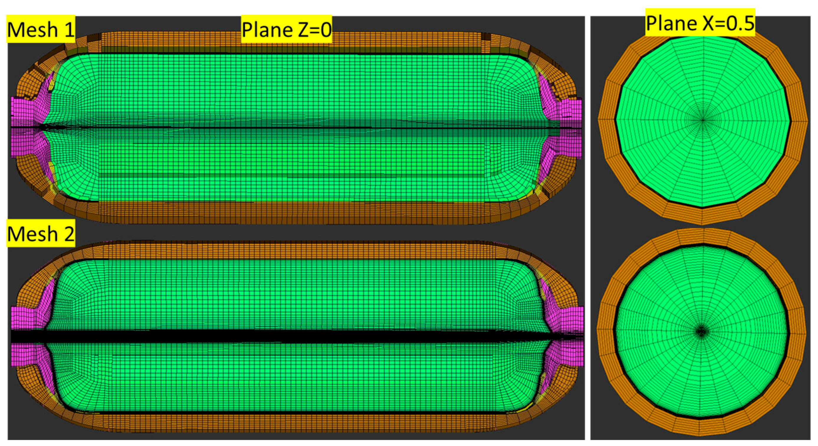
3.1. Calculation Domain and Numerical Mesh

The longitudinal and transversal cuts of the mesh of the 29 L Type IV tank are shown in Figure 2. One of the targets of the meshing strategy was to reduce the number of CVs while maintaining a reasonable mesh quality.

To improve the mesh quality, the boundary surface between the boss and the liner is slightly simplified, which should not influence the flow and temperature fields inside the tank. Two types of mesh are designed for the mesh sensitivity study. Mesh#1 is a uniform mesh with 95,000 hexahedral CVs. There are 10 CVs across the inlet pipe diameter of 3 mm, making a CV of 0.3 mm size, which represents the minimum cell size in such a mesh. Mesh#1-level 2 represents the global grid refinement of Mesh#1, which divides each cell by two in all three directions. Mesh#2 increases the density of CVs in all directions with a finer mesh (minimum size of about 0.1 mm) near the gas-solid boundary with about 260,000 hexahedral CVs. There are 28 CVs across the inlet pipe diameter in Mesh#2. The number of CVs and wall distance $y^{+}$ information are shown in

Table 2. The number of CVs, faces, and nodes for each mesh.

Mesh Name	CVs	$\mathbf{Maximum}\mathbf{Wall}{\mathit{y}}^{\mathbf{+}}$
		In Pipe	In Tank
Mesh#1	94,720	500–2000	50–500
Mesh#1-level 2	752,960	250–1000	25–250
Mesh#2	259,200	100–500	2–10

. For all meshes, the minimum orthogonal quality of CVs in fluid regions is 0.3–0.4, while 90% of CVs have a quality of 0.6–1.0. During the simulations with Mesh#1, the value of the maximum wall distance $y^{+}$ varies between 500 and 2000 in the pipe and 50 and 500 in the tank, while with Mesh#2, $y^{+}$ varies between 100 and 500 in the pipe and 2 and 10 in the tank for all turbulence models. Wall distance $y^{+}$ in the adopted meshes is acceptable for RANS with wall functions and hybrid models with near-wall treatment. For the LES simulations with Mesh#2, the wall distance y⁺ ≈ 2–10 falls within the buffer sublayer and the near-wall treatment blending laminar and logarithmic law-of-the-wall is employed.

3.2. Governing Equations

The governing conservation equations for the mass, momentum, and total energy are presented below (Equations (1)–(3), respectively). The expression of the total energy is presented by Equation (4). Equation (5) describes the contribution of turbulence to the thermal conductivity. In the RANS framework, Equations (1)–(3) are mass-weighted (Favre average) time-averaged equations [34], and in the LES framework, they are mass-weighted filtered equations [35]:

$$\frac{\partial \overline{\rho }}{\partial t}+\frac{\partial (\overline{\rho }{\tilde{u}}_i)}{\partial x_i}=0$$

(1)

$$\frac{\partial \left(\overline{\rho }{\tilde{u}}_i\right)}{\partial t}+\frac{\partial (\overline{\rho }{\tilde{u}}_j{\tilde{u}}_i)}{\partial x_j}=-\frac{\partial \overline{p}}{\partial x_i}+\frac{\partial }{\partial x_j}\left[\mu \cdot (\frac{\partial {\tilde{u}}_i}{\partial x_j}+\frac{\partial {\tilde{u}}_j}{\partial x_i}-\frac{2}{3}\frac{\partial {\tilde{u}}_k}{\partial x_k}{\delta }_{ij})\right]+\frac{\partial }{\partial x_j}({\overline{\tau }}_{ji})+\overline{\rho }{g}_i$$

(2)

$$\frac{\partial \left(\overline{\rho }\tilde{E}\right)}{\partial t}+\frac{\partial ({\tilde{u}}_i(\overline{\rho }\tilde{E}+\tilde{p}))}{\partial x_i}=\frac{\partial }{\partial x_j}\left[(k_g+{k_g}_t)\frac{\partial \tilde{T}}{\partial x_j}+{\tilde{u}}_i(\mu +{\mu }_t)(\frac{\partial {\tilde{u}}_i}{\partial x_j}+\frac{\partial {\tilde{u}}_j}{\partial x_i}-\frac{2}{3}\frac{\partial {\tilde{u}}_k}{\partial x_k}{\delta }_{ij})\right]+S_E$$

(3)

$$\tilde{E}=\tilde{h}-\frac{\overline{p}}{\overline{\rho }}+\frac{{\tilde{u}}^2}{2}$$

(4)

$$k_{g_t}=\frac{C_p{\mu }_t}{{\mathit{Pr}}_t}$$

(5)

Mass-weighted averaging and mass-weighted filtering are mathematically different procedures. However, after the introduction of turbulent viscosity (RANS) and subgrid-scale viscosity (LES), both the RANS governing equations (used for k-ε and k-ω models) and LES governing equations become formally identical. The difference lies exclusively in the size of the eddy viscosity provided by the underlying turbulence or subgrid-scale viscosity model. For the turbulent convective heat transfer, the concept of Reynolds’ analogy to turbulent momentum transfer is employed [36].

3.3. k-ε Model with a Modified Coefficient [37]

The standard k-ε model, proposed by Launder and Spalding [38], is based on model transport equations for the turbulent kinetic energy (k) and its dissipation rate (ε). As shown below, the Reynolds stress ${\overline{\tau }}_{ji}$ is described by a homogeneous turbulence viscosity based on the Boussinesq eddy-viscosity hypothesis [39]. It is a semi-empirical model, and the derivation of the model equations relies on phenomenological considerations and empiricism. Due to its robustness, economy, and reasonable accuracy, the k-ε model has been widely applied in industrial flow and heat transfer simulations. In the derivation of the k-ε model, the assumption is that the flow is fully turbulent, and the effects of the molecular viscosity are negligible, and it is therefore valid only for fully turbulent flows.

$${\overline{\tau }}_{ji}=-\rho \overline{u_i^{\prime }{u}_j^{\prime }}={\mu }_t\cdot (\frac{\partial u_i}{\partial x_j}+\frac{\partial u_j}{\partial x_i}-\frac{2}{3}\frac{\partial u_k}{\partial x_k}{\delta }_{ij})-\frac{2}{3}\rho k{\delta }_{ij}$$

(6)

$${\mu }_t=\rho C_{\mu }\frac{k^2}{\epsilon }$$

(7)

$$\frac{\partial \left(\rho k\right)}{\partial t}+\frac{\partial (\rho k{u}_i)}{\partial x_i}=\frac{\partial }{\partial x_j}\left[(\mu +\frac{{\mu }_t}{{\sigma }_k})\frac{\partial k}{\partial x_j}\right]+G_k+G_b-\rho \epsilon -Y_M+S_k$$

(8)

$$\frac{\partial \left(\rho \epsilon \right)}{\partial t}+\frac{\partial (\rho \epsilon u_i)}{\partial x_i}=\frac{\partial }{\partial x_j}\left[(\mu +\frac{{\mu }_t}{{\sigma }_{\epsilon }})\frac{\partial \epsilon }{\partial x_j}\right]+C_{1\epsilon }\frac{\epsilon }{k}(G_k+C_{3\epsilon }{G}_b)-C_{2\epsilon }\rho \frac{{\epsilon }^2}{k}+S_{\epsilon }$$

(9)

Different from the standard k-ε model, the coefficient $C_{1\epsilon }$ has a value of 1.52 (the standard value was 1.44) as suggested by Dicken and Mérida [37].

3.4. Reynolds Stress Model (RSM)

The Reynolds stress model, also referred to as second-moment closures, is the most complete classical turbulence model. In this model, the eddy-viscosity hypothesis is avoided, and the individual components of the Reynolds stress tensor (${\tau }_{ji}=-\rho \overline{u_i^{\prime }{u}_j^{\prime }}$) are directly computed. These models use the exact Reynolds stress transport equation for their formulation. They account for the directional effects of the Reynolds stresses and the complex interactions in turbulent flows. Reynolds stress models are expected to offer significantly better accuracy than eddy-viscosity-based turbulence models like k-ε models while being computationally cheaper than LES.

The transport equation of Reynolds stresses is shown below.

$$\begin{gathered} \frac{\partial \left(\rho \overline{u_i^{\prime }{u}_j^{\prime }}\right)}{\partial t}+\underset{C_{ij}\equiv \mathrm{Convection}}{\underbrace{\frac{\partial (\rho u_k\overline{u_i^{\prime }{u}_j^{\prime }})}{\partial x_k}}}=\underset{D_{T,ij}\equiv \mathrm{Turbulent}\mathrm{Diffusion}}{\underbrace{-\frac{\partial }{\partial x_k}\left[\rho \overline{u_i^{\prime }{u}_j^{\prime }{u}_k^{\prime }}+p^{\prime }({\delta }_{kj}{u}_i^{\prime }+{\delta }_{ik}{u}_j^{\prime })\right]}}+\underset{D_{L,ij}\equiv \mathrm{Molecular}\mathrm{Diffusion}}{\underbrace{\frac{\partial }{\partial x_k}\left[\mu \frac{\partial \left(\overline{u_i^{\prime }{u}_j^{\prime }}\right)}{\partial x_k}\right]}} \\ -\underset{P_{ij}\equiv \mathrm{Stress}\mathrm{Production}}{\underbrace{\rho \left(\overline{u_i^{\prime }{u}_k^{\prime }}\frac{\partial u_j}{\partial x_k}+\overline{u_j^{\prime }{u}_k^{\prime }}\frac{\partial u_i}{\partial x_k}\right)}}\underset{G_{ij}\equiv \mathrm{Buoyancy}\mathrm{Production}}{\underbrace{-\rho \beta \left(g_i\overline{u_j^{\prime }\theta }+g_j\overline{u_i^{\prime }\theta }\right)}}+\underset{{\varphi }_{ij}\equiv \mathrm{Pressure}\mathrm{Strain}}{\underbrace{\overline{p^{\prime }(\frac{\partial u_i^{\prime }}{\partial x_j}+\frac{\partial u_j^{\prime }}{\partial x_i})}}} \\ \underset{{\epsilon }_{ij}\equiv \mathrm{Dissipation}}{\underbrace{-2\mu \overline{\frac{\partial u_i^{\prime }}{\partial x_k}\frac{\partial u_j^{\prime }}{\partial x_k}}}}\underset{F_{ij}\equiv \mathrm{Production}\mathrm{by}\mathrm{System}\mathrm{Rot}\mathrm{a}\mathrm{tion}}{\underbrace{-2\rho {\Omega }_k\left(\overline{u_j^{\prime }{u}_m^{\prime }}{\epsilon }_{ikm}+\overline{u_i^{\prime }{u}_m^{\prime }}{\epsilon }_{jkm}\right)}} \end{gathered}$$

(10)

The terms $C_{ij}$, $D_{L,ij}$, $P_{ij}$, and $F_{ij}$ in Equation (10) can be computed directly without modelling and the terms $D_{T,ij}$, $G_{ij}$, ${\varphi }_{ij}$, and ${\epsilon }_{ij}$ still need to be modelled to close the equations. In this paper, we use the ANSYS Fluent realisation of the ε-based RSM [40] with a linear pressure–strain model.

3.5. Large Eddy Simulation (LES)

The idea of LES is to reduce the computational cost compared to Direct Numerical Simulation (DNS). While resolving large scales comparable with the mesh size, LES models the unresolved scales at the subgrid level. Contrary to RANS, where turbulent motion is averaged across all scales, the LES approach relies on the resolution of the largest, non-isotropic and energy-containing eddies, and models only relatively small and isotropic ones. As a result, the large flow structures are computed directly, providing an instantaneous field and better solution for non-isotropic turbulent flows. The downside of LES is more stringent requirements for numerical grid and time steps, usually leading to longer CPU times.

The mass-weighted filtered equations for the mass, momentum, and energy equations look the same as those for the RANS Favre-averaged Equations (1)–(3). Their main difference is in the expression of the eddy viscosity provided by the turbulence models. The finite-volume discretisation method itself may be considered an LES box filter. In this paper, we use the Dynamic Smagorinsky–Lilly Model for the subgrid-scale viscosity [41]:

$${\mu }_t=\rho L_s^2\sqrt{2{\overline{S}}_{ij}{\overline{S}}_{ij}}$$

(11)

$$L_S=\mathit{min}(0.41d,C_S{V}^{1/3})$$

(12)

3.6. Detached Eddy Simulation (DES) [42]

Detached eddy simulation (DES) is a modification of the RANS approach in which the model switches to an LES simulation in regions where the turbulent length scale exceeds the grid size. For the “grey area” [43] between those two treatments, a DES modification in the SST model is applied to the dissipation term in the k-equation. This process is performed by an approximate modification of the turbulence length scale parameter, which is, explicitly or implicitly, involved in the RANS turbulence model [44]. This allows us to avoid the high-resolution requirements for wall boundary layers. Here, the k-ω SST model [26] is chosen as the RANS model underlying DES.

However, as the model transition includes a grid size, users may encounter grid spacings that disturb the RANS model. When the grid spacing parallel to the wall becomes smaller than the boundary-layer thickness, the DES length scale follows the LES branch, though does not resolve boundary-layer turbulence. Therefore, the modelled Reynolds stress is reduced without any sizeable, resolved stress to restore the balance, which is referred to as modelled-stress depletion (MSD). To address this deficiency, a new version of this technique, known as Delayed Detached Eddy Simulation (DDES) [45], is applied here based on a simple modification to DES.

3.7. Scale-Adaptive Simulation (SAS) [28]

The SAS concept is based on the introduction of the von Kármán length scale into the turbulence scale equation. The information provided by the von Kármán length scale allows SAS models to dynamically adjust to resolved structures in unsteady RANS simulations (URANS), which results in an LES-like behaviour in unsteady regions of the flow field. At the same time, the model provides standard RANS capabilities in stable flow regions. The SAS model can reduce the turbulent viscosity by adding a term to increase the production term in the ω-equation, instead of increasing the dissipation term in the k-equation in the DES approach [46]. SAS models behave in many situations similar to DES models but without the explicit influence of the grid resolution on RANS simulations. This allows for a safer passage from RANS to Scale-Resolving Simulation, especially for complex applications, where high-quality ”LES-meshes” cannot easily be generated for the detached flow regions [47].

3.8. Initial and Boundary Conditions

The initial and boundary conditions for the simulations are based on the fuelling experiment described in [13]. The initial temperature and pressure in the tank are 303.15 K and 2.0 MPa, respectively. The inlet hydrogen temperature is 273.15 K. The experimental inlet pressure history [13] is approximated in simulations via a sixth-order polynomial and is used as the inlet boundary condition. A non-slip boundary condition is applied on all solid surfaces. The conjugate heat transfer approach has been used to describe heat transfer through solid materials coupled with the changing temperature in the fluid. The heat transfer coefficient on the outer surface of the tank is assumed to be 6 W/K/m² [19].

The authors of the study [13] measured a pressure jump of around 5 MPa at the first second of fuelling, which is 10 times the global average pressure ramp. A similar difference between the measured inlet pressure and pressure inside the tank at the beginning of fuelling can also be observed in another JRC test [48]. This could be due to peculiarities of pressure measuring at the start of the fuelling. To avoid numerical instability and solution divergence, a smoothed pressure ramp was introduced for the first 10 s at the inflow boundary in the CFD simulations, which reduced this pressure jump.

3.9. Numerical Details

ANSYS Fluent 20.2 was used as a computational engine. The Pressure-Implicit with Splitting of Operators (PISO) scheme is applied as the pressure–velocity coupling method. A bounded second-order implicit scheme is chosen for time discretisation. A second-order upwind scheme is chosen for spatial discretisation. Five turbulence models, i.e., modified k-ε model, RSM, LES, SAS, and DES, are compared regarding the accuracy of reproducing the experimental averaged temperature transient and spatial distribution of parameters in the simulations. The Redlich–Kwong equation of state for real gas [49] is applied in all models as its accuracy has been proved by Miguel et al. [13] with the same validation experiments. The simulation started with a small time step of 10⁻⁵ s, and then gradually increased by a factor of 1.005 after each time step until reaching the allowed maximum time step (see

Table 3. Simulation cases and characteristic calculation speed.

Case	Turbulence Model	Mesh *	Maximum Time Step (s)	Solution Time per Iteration (s)				Speed
				Mass and Momentum Equations	Turbulence Model Equations	Energy Equation	CPU Time	Simulation Time/CPU Time (s/hour)
#1	Modified k-ε	Mesh#1	0.004	0.038	0.004	0.007	0.051	14.1
#2	Modified k-ε	Mesh#1-level 2	0.002	0.144	0.033	0.043	0.228	1.58
#3	Modified k-ε	Mesh#1	0.0004	0.019	0.003	0.007	0.032	2.25
#4	RSM	Mesh#1	0.0004	0.017	0.008	0.007	0.035	2.06
#5	DES	Mesh#1	0.0004	0.021	0.007	0.007	0.038	1.89
#6	SAS	Mesh#1	0.0004	0.019	0.008	0.008	0.040	1.80
#7	LES	Mesh#1	0.0004	0.014	N/A	0.008	0.026	2.77
#8	LES	Mesh#2	0.0001	0.046	N/A	0.019	0.077	0.234

Notes: *—Mesh#1 has 94,720 CVs; Mesh#1-level 2—752,960 CVs; Mesh#2—259,200.

). The solution convergence of the linear equations was controlled by requiring all residuals to be below the 10⁻³ threshold. The continuity equation residual was the last to reach this 10⁻³ condition. The momentum conservation equation residual reached a value around 10⁻⁶ at the same time. The influence of the residual level on the temperature dynamics was found to be within 1% after further decreasing the continuity equation residual down to 10⁻⁴ (this increased the simulation time by around 30%). The hydrogen mass imbalance was within 0.1% only.

4. Results and Discussion

4.1. Simulation Speed

Table 3 shows the list of performed simulations with different turbulence models, numerical grids, and time steps together with the CPU time required for the solution of one iteration of the individual conservation equations and one iteration for the overall system solution.

The allowed maximum time step was chosen to achieve the target equation residuals within 10–30 iterations per time step while keeping the overall CPU time at a minimum. For Cases #3–#7, the maximum CFL number is 200–400 in the pipe and 10–30 in the central region of the jet at the start of the fuelling simulations. By the end of the fuelling simulations, the maximum CFL is 20–40 in the pipe and 1–3 in the central region of the jet. The CFL number is always below 1 in the near-wall region. In Case #8, the refined mesh and reduced time step resulted in a CFL below 1 for 95% of CVs at a fuelling time of 30 s, which allows LES to simulate turbulent motion resolvable on the grid.

To speed up the simulations, the time step (and CFL number) was increased by 10 times with the k-ε model in Case#1. Case#2 is a global mesh refinement based on Case#1 with the same CFL. Such a choice of CFL value was considered reasonable to speed up the simulations and achieve a convergence of the conservation equations, particularly in combination with a relatively stable jet flow and a stable implicit CFD solver.

All demonstrated solution times were obtained using 64 cores on a Dell PowerEdge R6525 workstation equipped with two AMD EPYC 7702 64-core processors (providing 128 cores in total). The calculation speed for each case was obtained by scaling the calculation time of 20 time steps with 30 iterations per time step (600 iterations). Each case was run twice or more, and the time variation for different runs was within 5%. The time step size during this speed test is equal to its maximum value during simulations. The overall CPU time per iteration represents the sum of times to solve the mass and momentum conservation equations, turbulence model equations, energy conservation equations, and other auxiliary calculations. No turbulence model solutions are recorded for LES as no transport equations for turbulence parameters are solved.

For Cases #3–#7 with the same time step and mesh, LES shows the shortest time of 0.026 s for each iteration while others require 0.032–0.040 s (the accuracy of the reproduction of the experimental data will be discussed later). This is because LES does not solve additional turbulence model equations as other models do. The solution time for the energy equation is similar for all cases independent of the time step size and is proportional to the total CV number used in a particular mesh. The solution time for the mass and momentum conservation equations is influenced by the choice of time step (associated with the choice of turbulence model): Cases #1 and #2 have this time increased significantly with increasing time steps. Based on the simulation time usage reported by Fluent, a longer solution time was required by the linear equations solver in these cases. This may be due to a larger residual of the mass and momentum conservation equations produced by a larger time step.

The overall low CPU time per iteration for the LES models could mislead and give the notion that the LES model is the fastest of all the turbulence modelling approaches. While the choice of turbulence model affects the simulation speed within 50%, the LES model required an order of magnitude lower time step, which resulted in a five times slower calculation speed compared to the modified k-ε model with the same Mesh#1. Between models using the same Mesh#1 and the same time step of 0.0004 s, the LES model provided the fastest calculation speed. Based on the simulation results, the RANS models can allow a larger time step. The RANS cases with the modified k-ε turbulence model may be simulated with a time step of 0.004 s (a maximum time step of 0.020 s has been used by Melideo et al. [19] with the k-ω SST model). To resolve even the largest energy-containing eddies, the LES model requires a finer mesh and a smaller time step. For Case #8, the maximum time step size is limited to 0.0001 s to reduce the continuity residual below 10⁻³. The continuity residual larger than 0.01 led to an unacceptable accumulation of apparent local and global mass imbalance in the simulations. As a result, with the time step of 0.004 s, the speed of the modified k-ε turbulence model is 60 times faster than the LES model, as shown in Table 3. In practice, there will be differences in the iteration numbers for each time step. Overall, to finish the fuelling simulation of 190 s duration, as in the experiment, the Case #1 simulation is the fastest and takes only 3 days on 64 cores, while Case #8 is the slowest and takes more than 1 month on 128 cores.

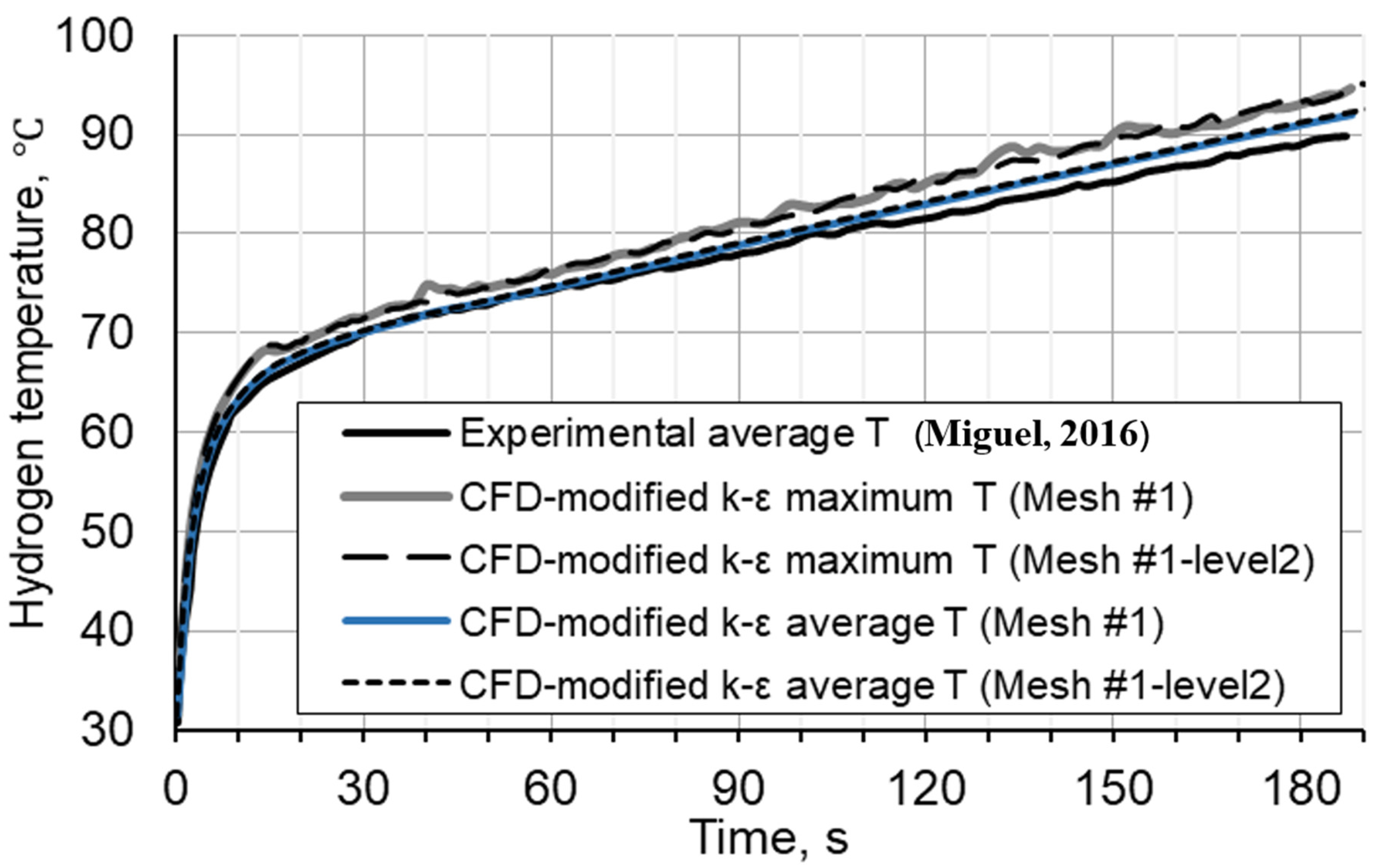
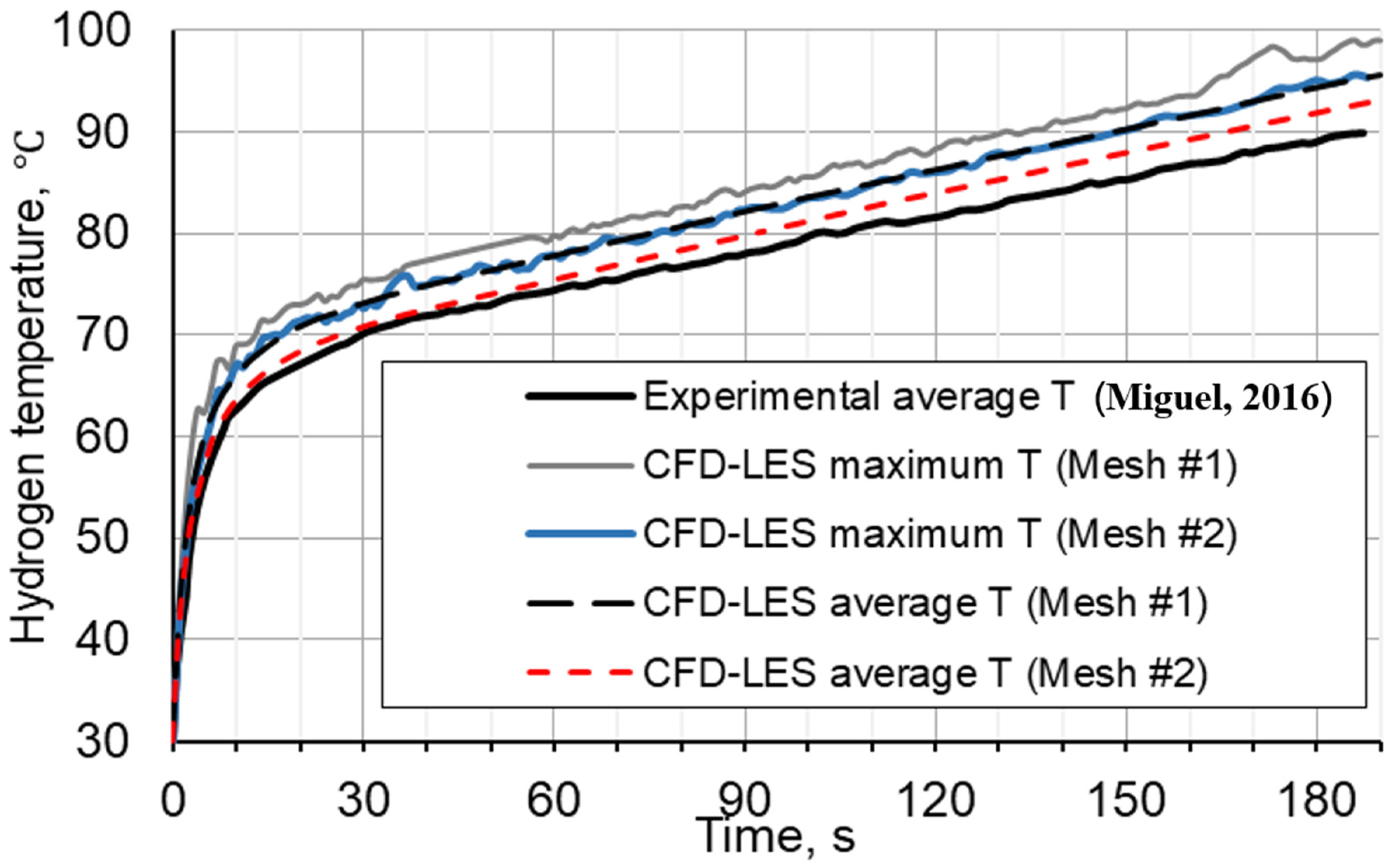
4.2. Grid Sensitivity

The grid sensitivity study was performed only for two models, i.e., modified k-ε and LES, due to limited computational resources. Figure 3 and Figure 4 represent the hydrogen temperatures using mass-averaged and maximum temperature dynamics in the tank as the results of the simulations with different meshes.

For the modified k-ε model, the mesh density in the original Mesh#1 is doubled everywhere in Mesh#1-level 2, reducing the maximum wall $y^{+}$ from 50–500 to 25–250. It can be seen in Figure 3 that there is no difference between the average temperature histories (blue bold and black short-dash curves) while differences of up to 3% can be observed between the maximum temperature histories (grey bold and black long-dash curves).

Figure 4 demonstrates that the results of the solutions with the LES model, such as temperatures, are more sensitive to meshes than those with the RANS models.

It can be seen in Figure 4 that Mesh#1 (maximum wall $y^{+}$ = 50–500 in tank) gives a larger overprediction of the average temperature, i.e., by 6% (black bold and blue curves). The simulation results become closer to the experimental value with a difference of up to 3% (black bold and red dashed curves) when using Mesh#2 with a maximum wall $y^{+}$ = 2–10 in tank.

In the following discussion, Case #1 and Cases #4–8 in Table 3 are simulated through the whole fuelling process. The same maximum time step sizes as shown in Table 3 were used. For convenience of discussion, they will be referred to by turbulence model and mesh.

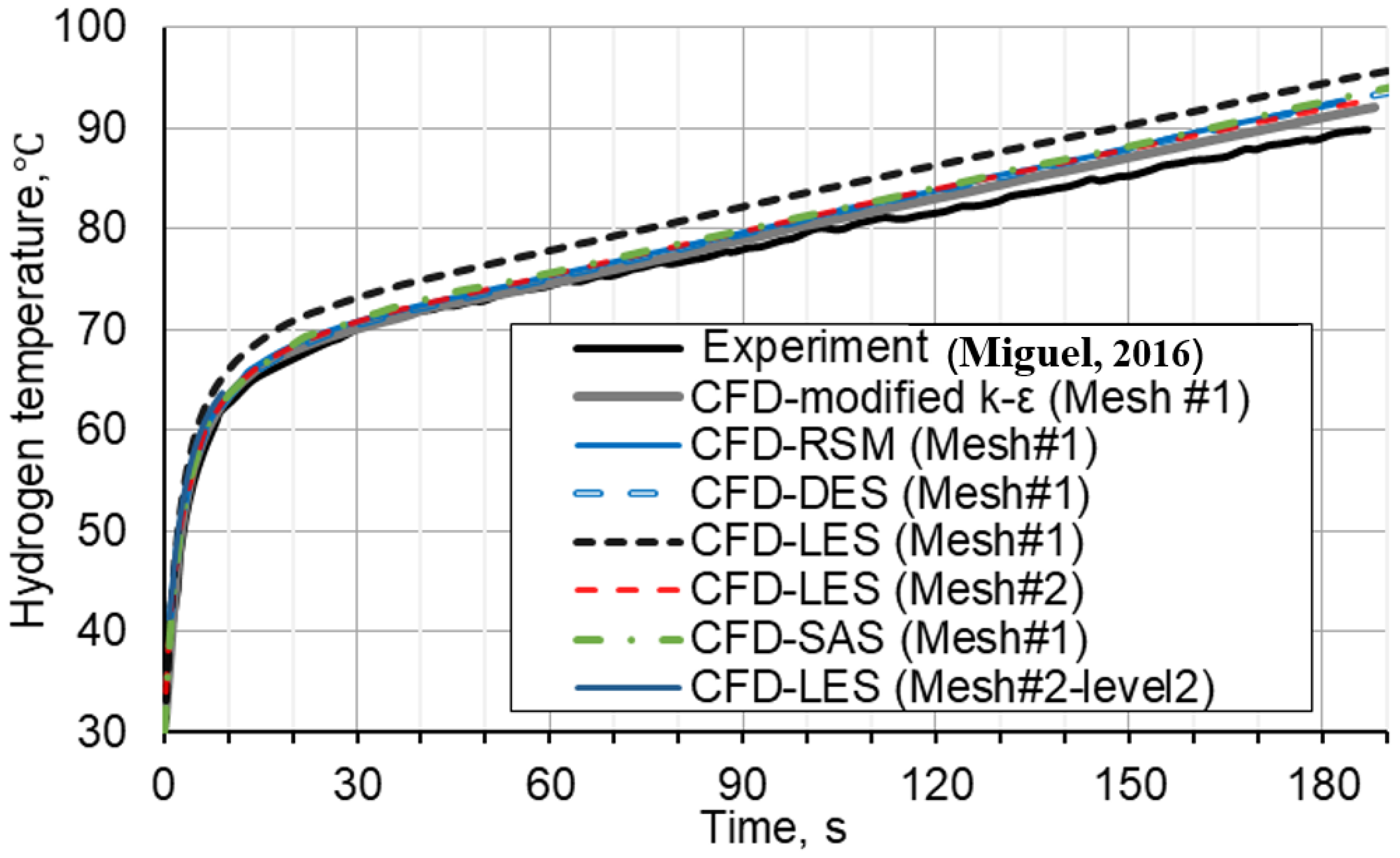
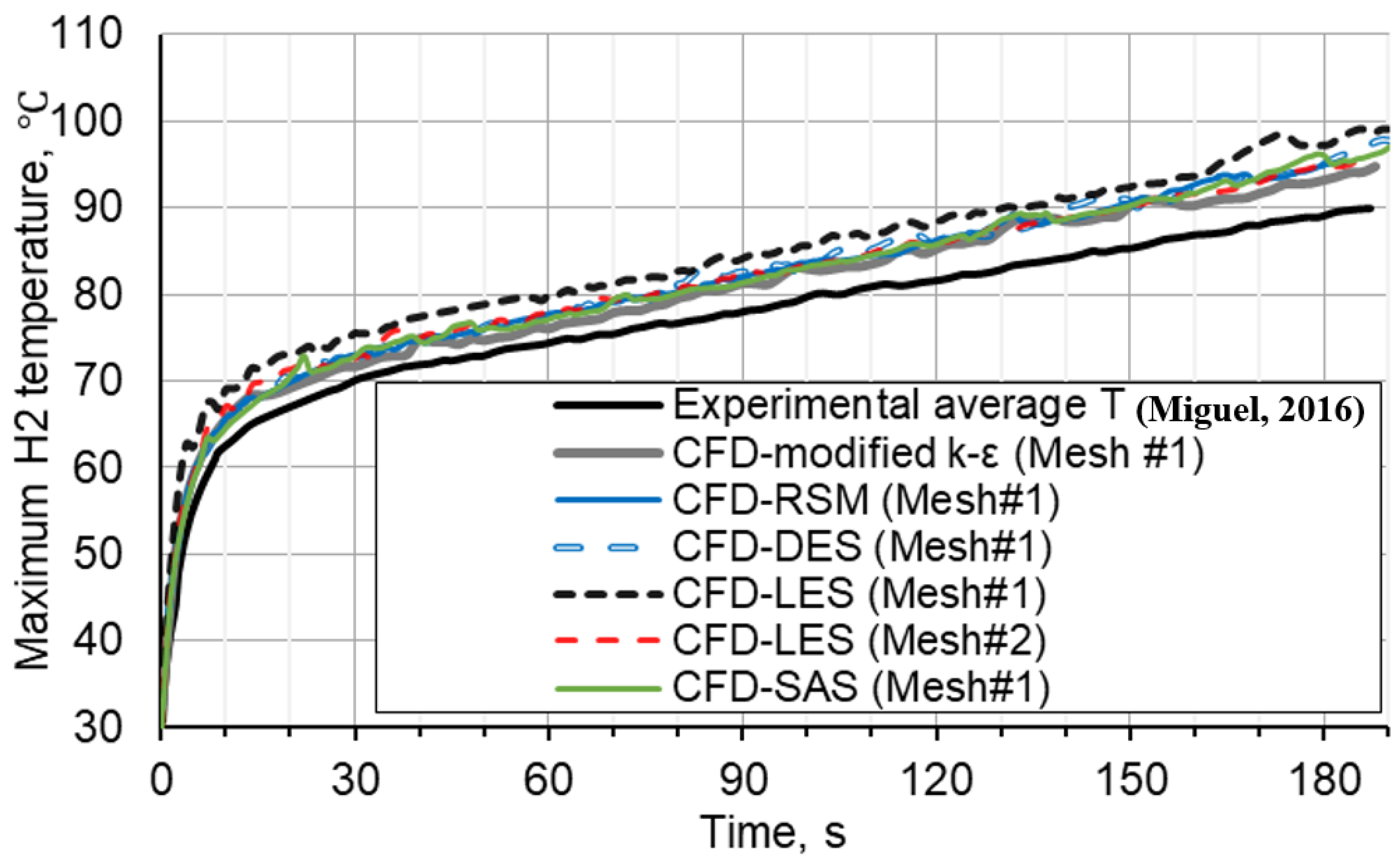
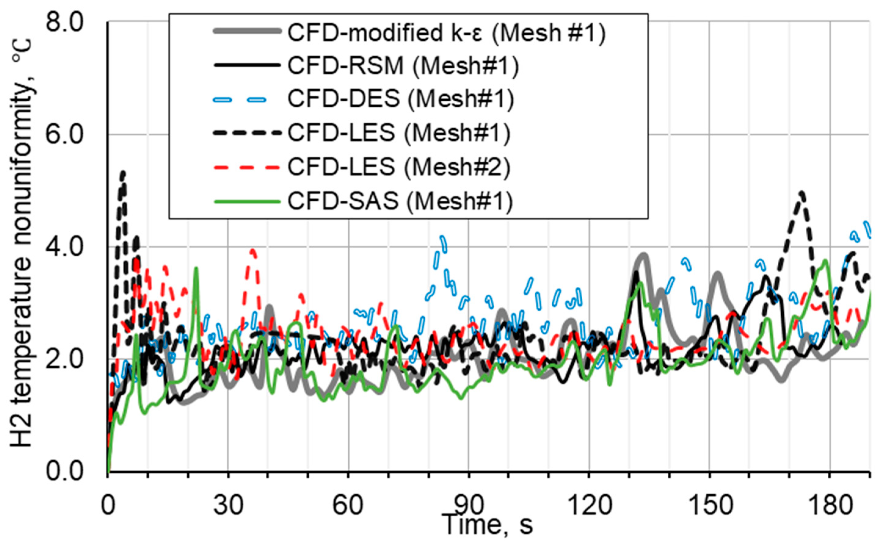
4.3. Hydrogen Temperature inside the Tank

Figure 5 shows the average temperature history of the experiment. The difference between the modified k-ε (Mesh#1), RSM (Mesh#1), DES (Mesh#1), SAS (Mesh#1), and LES (Mesh#2) models is within 1%. All models can produce results close to the experimental average hydrogen temperature.

It can be concluded in Figure 5 that only LES (Mesh#1) shows an apparent deviation of up to 5 degrees (6%). For the rest of the cases, the maximum deviation from the experiment is within 2–3 degrees (within 3%), i.e., comparable with the experimental accuracy of the temperature measurements. The reason that LES (Mesh#1) has larger errors is possibly due to two reasons: the time step size of 0.0004 s is still large, which increases the numerical error; the coarse grid near the wall ($y^{+}$ > 50) underestimates the heat flux to the wall. It can be confirmed by the improved results in LES (Mesh#2), where the time step size and maximum wall $y^{+}$ are reduced to 0.0001 s and 2–10 in the tank, respectively.

Figure 6 shows the comparison of the maximum temperature dynamics in the tank between different simulations. In its major features, the maximum temperature dynamics follow the same trend as the average one in Figure 5: the temperature in the simulations with LES (Mesh#2) is the largest and the modified k-ε (Mesh#1) is the smallest, with the rest of the models closely following each other in between those two.

Figure 7 shows the difference between the maximum and average simulated gas temperatures.

All modelling approaches predict a relatively uniform temperature distribution inside the tank with temperature differences as low as 1–5 degrees during the entire fuelling. A relatively uniform temperature is expected in this L/D~3 vessel. It is thought to be due to the well-established recirculating flow throughout the tank that can be seen from our further analysis.

However, it may be noticed that the DES and SAS models may overpredict the temperature gradient inside the tank. In our first simulations (not shown here), first-order schemes were used by default for the k and ω transport equations in Fluent. When the simulation approached 190 s, the temperature non-uniformity increased quickly to 6 degrees and 12 degrees in simulations with the SAS and DES models, respectively. After second-order schemes were applied, those temperature non-uniformities disappeared. On the contrary, the modified k-ε models and RSM models are not sensitive to the numerical scheme order. The simulations with LES do not demonstrate such an issue as no additional transportation equations are solved. It shows that the SAS and DES models are more sensitive to grid resolution than other models and should be used carefully.

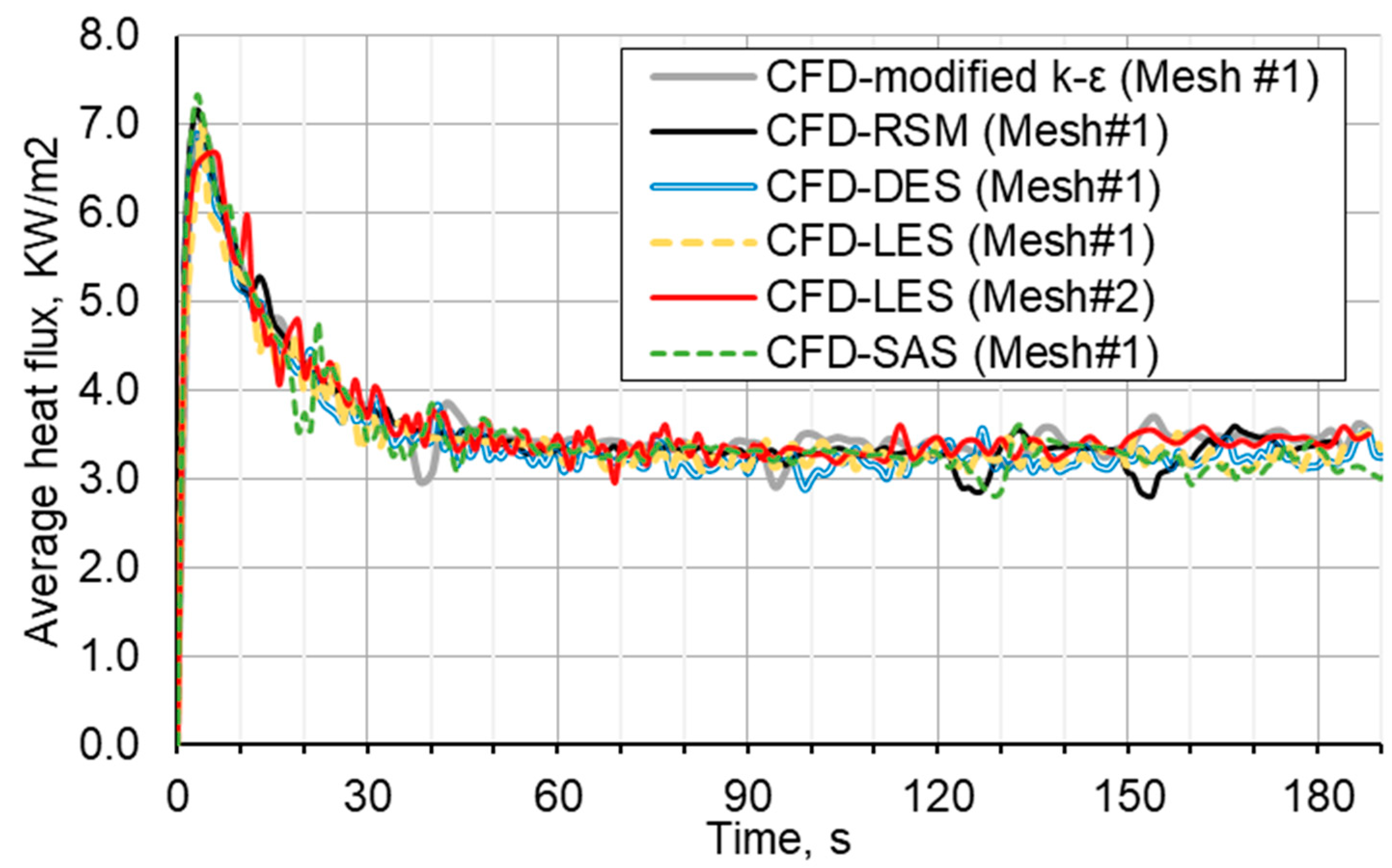
4.4. Heat Flux to the Tank

Figure 8 shows the dynamics of the average heat flux from hydrogen to the liner. It can be seen that the average values are close to each other with deviations of up to 15%. Here, we can see LES (Mesh #1) slightly underestimates the heat flux in the first 10 s (by 1–15%) while it has a larger hydrogen temperature than others. It explains why the bulk gas temperature is overestimated. The LES, SAS, and DES models are expected to resolve turbulent oscillations better compared to the RSM and modified k-ε models, hence more oscillating heat fluxes.

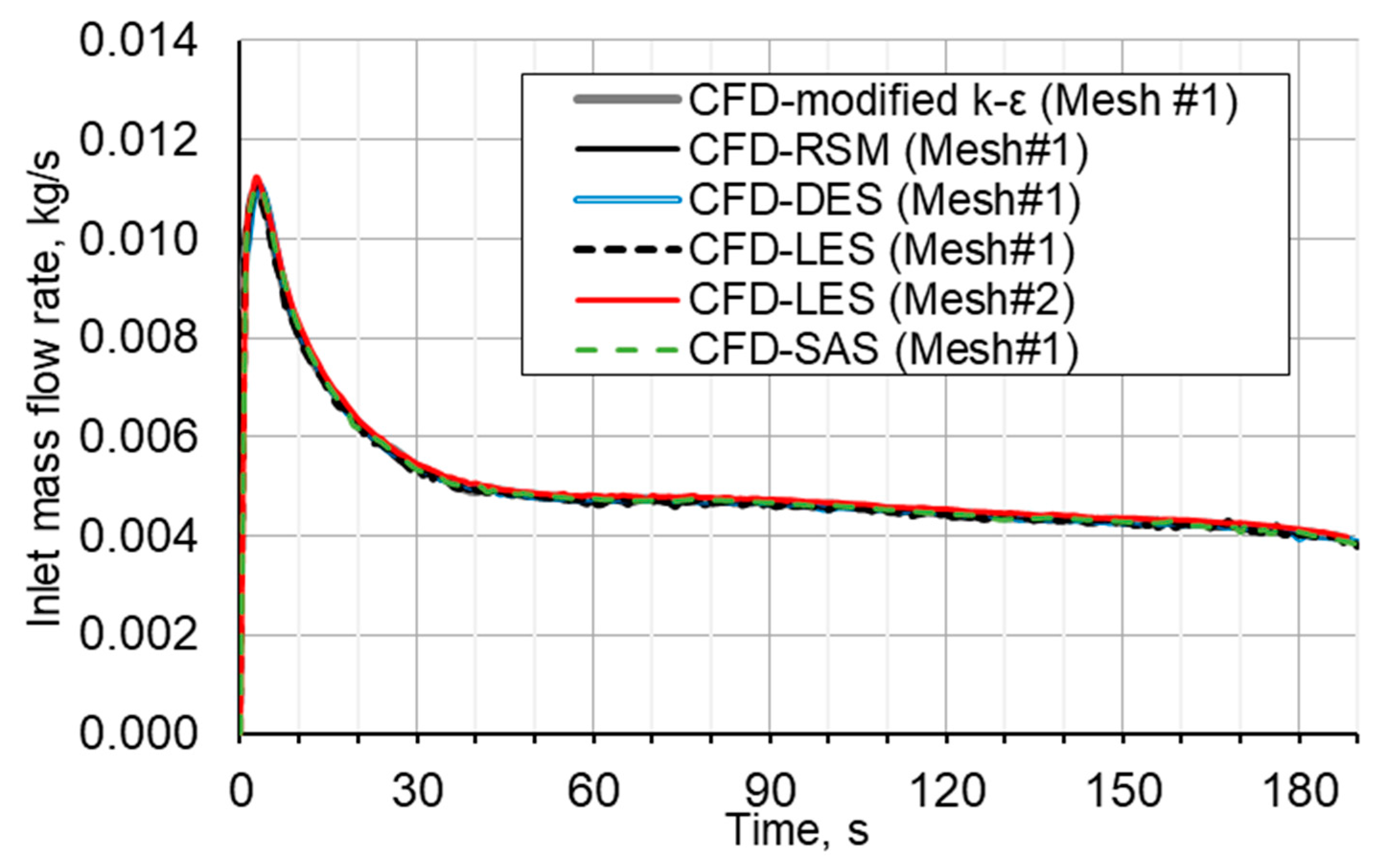
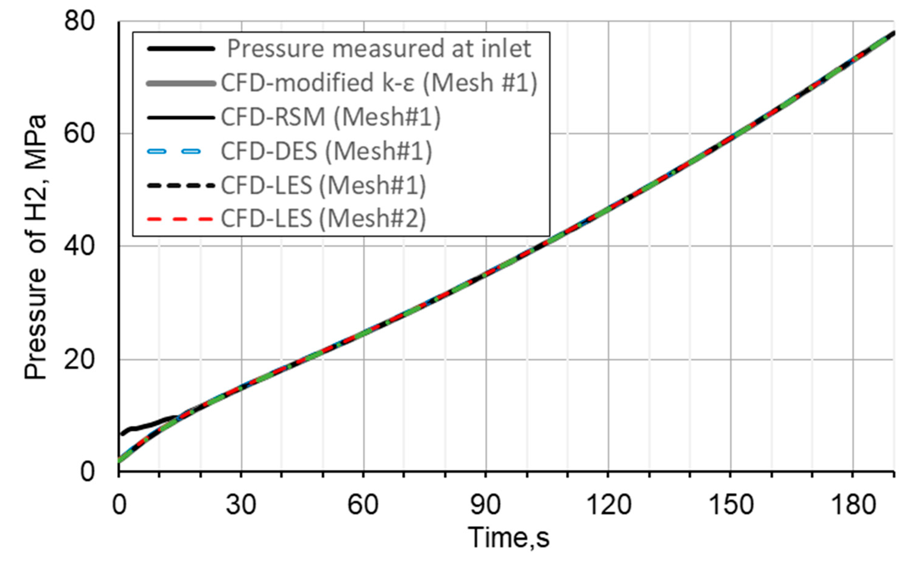
4.5. Pressure in the Tank and the Inlet Mass Flow Rate

Figure 9 and Figure 10 show the time dependence of the inlet mass flow rate and hydrogen pressure inside the tank, respectively. For the inlet mass flow rate, the difference between all models is around 1%.

The mass inflow rate is directly connected to the pressure inlet boundary conditions and the simulated hydrogen pressure inside the tank. As a result, such an integral parameter as simulated tank pressure is also identical between different models. Similar to Miguel et al. [13], it is observed that simulated pressures quickly approach the experimentally measured pressure at the inlet after 14 s.

The consistency of the inlet mass flow rate and gas pressure with the experimental values validates the pressure boundary condition and numerical schemes used in the simulations by all models. As discussed above, the difference between the inlet pressure and pressure inside the tank at the start of fuelling is due to the measurements with a sudden release of hydrogen. A similar difference between the measured inlet pressure and pressure inside the tank can be found in experiments [44].

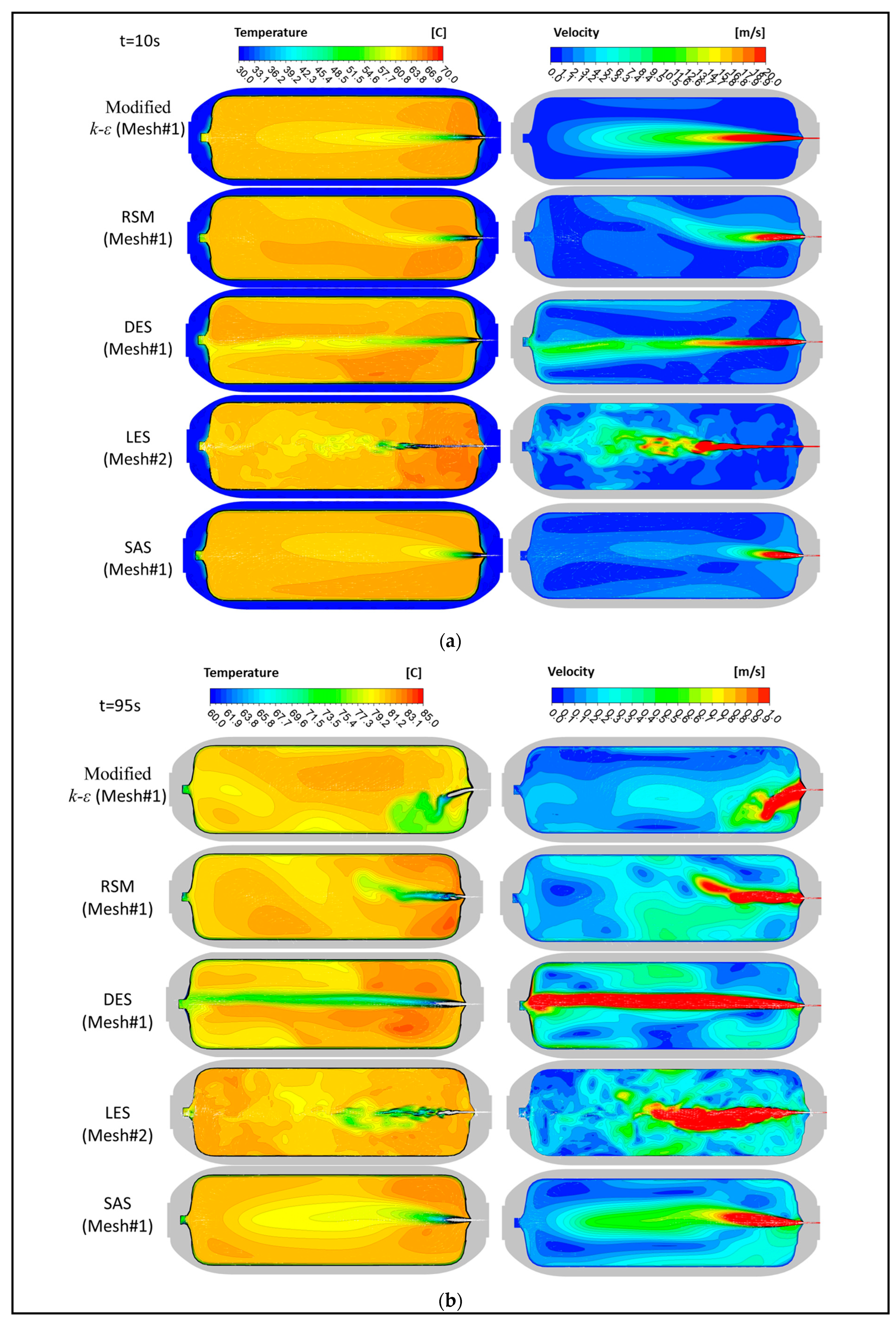
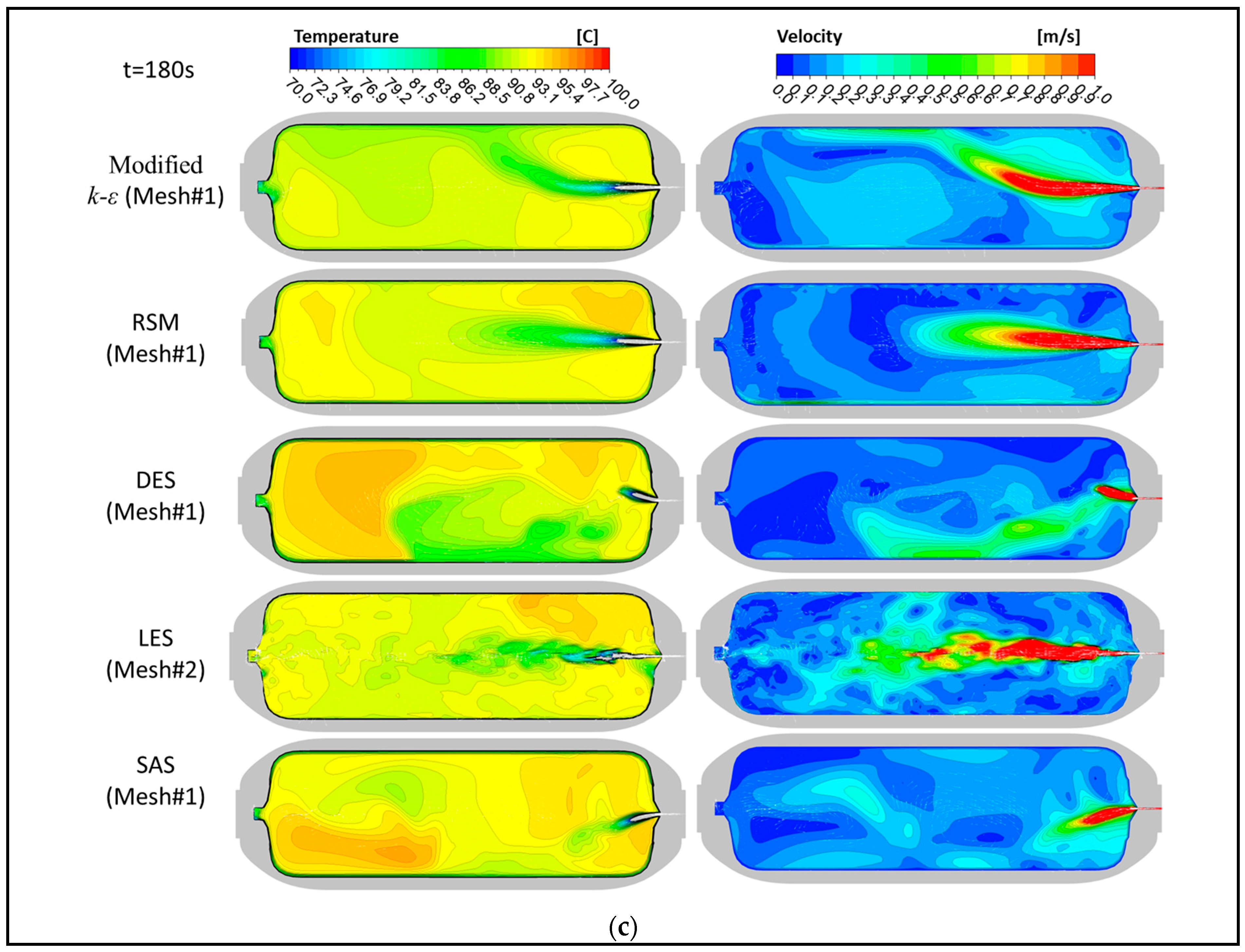
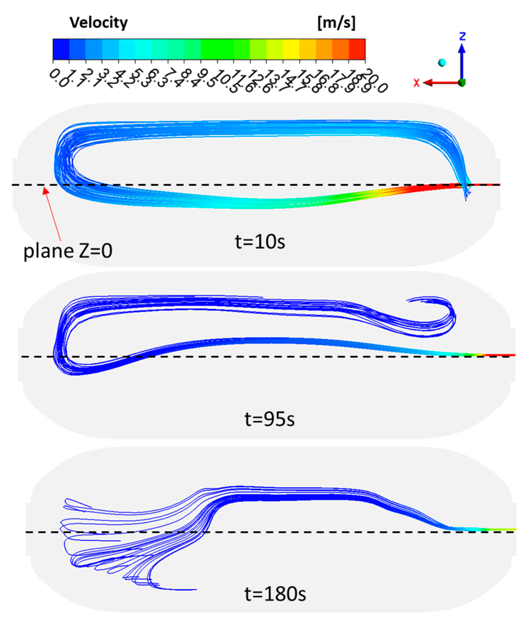
4.6. Velocity and Temperature Distributions inside the Tank

The transient velocity and temperature fields are shown in Figure 11 at times t = 10 s, t = 95 s, and t = 180 s.

It can be seen in Figure 11 that the transient flow and temperature distributions are different for all five models. For the modified k-ε model and RSM model, the flow is time-averaged, and no eddies are resolved. A clear interface between the jet and bulk fluid is found while the jet oscillates up and down around the tank axis. A similar phenomenon has been observed by Gonin et al. [2] with the k-ω SST model. A closer analysis of the results in this study revealed that the oscillations along the tank axis have a spatial three-dimensional nature, as shown in Figure 12, for the SAS model. A similar behaviour was observed for the DES simulation results as well. The jet fluctuation contributes to the mixing of cold gas and hot gas inside the tank, which significantly reduces the temperature non-uniformity.

The 3D nature of the flow makes it difficult to compare the results of different turbulence models in the same tank cross-section. For the LES model, large eddies are resolved in simulations directly (that is why LES requires a finer mesh and smaller time step than RANS). So, it gives more realistic and better-resolved vortexes during the hydrogen injection and jet development inside the tank. The spatial temperature distribution is no longer continuous, accompanied by vortexes originating from the main jet.

The DES model solves the RANS equations in the region near the walls while solving the LES equations in the rest of the domain. It significantly relaxes the LES model requirements for the mesh and time step while retaining the most LES model benefits. At the simulation time t = 10 s, the DES model shows a temperature and velocity distribution similar to that observed in the solution with the LES model. The velocity distribution in the jet is less dispersed in the simulation with the DES model than in the simulation with the LES model. At time t = 180 s, a horizontal temperature non-uniformity is particularly pronounced for the LES, SAS, and DES turbulence models.

For the modified k-ε model, the temperature distribution is the most uniform, which may be caused by the overprediction of viscosity as observed by Gonin et al. [2]. For the RSM model, the simulation results are generally close to those of the modified k-ε model. Yet, compared to the k-ε model, the flow field obtained with the RSM model results appears to be less uniform and captures the main characteristics of the flow and temperature fields of the LES model, which corresponds to a good balance between the simulation time and accuracy.

For the SAS model, the simulation result is close to the RANS result at the beginning of fuelling. This may be due to the use of the coarse grid. At time t = 180 s, the SAS results are halfway between RANS and LES, showing a quite pronounced temperature and velocity non-uniformity, though the maximum temperature and temperature gradient in the horizontal direction are lesser than those obtained with DES.

5. Conclusions

This paper focuses on the influence of the turbulence model choice on the CFD simulation of gaseous hydrogen fuelling. The high-pressure fuelling of a 29 L, type IV hydrogen tank was simulated using five different turbulence models.

The originality of this study is the direct comparison of different turbulence models’ performance in 3D CFD simulations of the same hydrogen fuelling process. For the first time, the fuelling simulations were performed with 3D LES and hybrid RANS–LES models (SAS and DES), as well as using RANS (modified k-ε model and RSM) models. This paper compares and analyses the simulation results using these models, particularly the hydrogen pressure, temperature, heat flux, and flow velocity in the tank, which had not been reported, in the context of hydrogen safety.

The significance of this work is in the provision of data for the informed choice of the turbulence model for practical hydrogen fuelling simulations in the context of tank design, safety analysis, fuelling protocol development, etc. The advantages and drawbacks of the five turbulence models are demonstrated and discussed. Different flow and temperature distributions are observed even though all models resulted in a similar average gas temperature and identical pressure dynamics in the tank. The k-ε model owns the advantages of robust simulations using coarse meshes and large CFL numbers (y⁺ > 100 and CFL >> 1), which allows the 190 s fuelling simulation to be finished in 3–4 days using a typical present-day workstation. The LES model requires a finer numerical mesh (y⁺~1) and CFL~1 to reproduce the experimental temperature history. LES simulation can take up to over 1 month of CPU time using the same computing hardware. However, it provides superior results compared to RANS in terms of the temperature and velocity non-uniformity inside the tank. The SAS and DES models allow for a coarser mesh than LES. Yet, both models can capture the main characteristics of flow and temperature distribution similar to the LES solution. Some artefacts observed in the SAS and DES simulations (e.g., the temperature gradient in the horizontal direction) cannot be validated due to a lack of detailed experimental measurements. Nonetheless, the hybrid LES–RANS models demonstrated their merits and are superior to RANS models’ capability, which prompts closer attention of the modelling community to those modelling approaches as potential design tools. The RSM has the benefit of a more fundamentally based model compared to the modified k-ε model, which potentially should result in more accurate and physically sound predictions in complex geometries. Considering the balance of accuracy and speed, both the SAS and RSM models are highly commendable and have a substantial potential for use in practical fuelling applications.

The rigour of this work is in the validation of the wide range of turbulence models against the available experimental data on the hydrogen temperature during high-pressure tank fuelling. A detailed analysis of the model choice and grid sensitivity on such design parameters as the temperature dynamics, temperature and velocity distribution, inlet mass flow rate, pressure history, and CPU time was performed.

References

1. Zheng, J.; Liu, X.; Xu, P.; Liu, P.; Zhao, Y.; Yang, J. Development of high pressure gaseous hydrogen storage technologies. Int. J. Hydrogen Energy 2012, 37, 1048–1057. [Google Scholar] [CrossRef]
2. Gonin, R.; Horgue, P.; Guibert, R.; Fabre, D.; Bourguet, R.; Ammouri, F.; Vyazmina, E. A computational fluid dynamic study of the filling of a gaseous hydrogen tank under two contrasted scenarios. Int. J. Hydrogen Energy 2022, 47, 23278–23292. [Google Scholar] [CrossRef]
3. Wang, X.; Tian, M.; Chen, X.; Xie, P.; Yang, J.; Chen, J.; Yang, W. Advances on materials design and manufacture technology of plastic liner of type IV hydrogen storage vessel. Int. J. Hydrogen Energy 2022, 47, 8382–8408. [Google Scholar] [CrossRef]
4. Gebhart, T.M.; Spiller, M.; Çelik, H.; Dahlmann, R.; Hopmann, C. Experimental analyses of the spatial varying temperature development of type-IV hydrogen pressure vessels in cyclic tests considering different length to diameter ratios. Int. J. Hydrogen Energy 2023, 48, 27304–27318. [Google Scholar] [CrossRef]
5. Li, M.; Bai, Y.; Zhang, C.; Song, Y.; Jiang, S.; Grouset, D.; Zhang, M. Review on the research of hydrogen storage system fast refueling in fuel cell vehicle. Int. J. Hydrogen Energy 2019, 44, 10677–10693. [Google Scholar] [CrossRef]
6. Society of Automotive Engineers J2601. Fueling Protocols for Light Duty Gaseous Hydrogen Surface Vehicle; SAE International: Warrendale, PA, USA, 2020. [Google Scholar]
7. Global Technical Regulation on Hydrogen and Fuel Cell Vehicles. Addendum 13: Global Technical Regulation No. 13. Global Registry; United Nations Economic Commission for Europe: Geneva, Switzerland, 2020. [Google Scholar]
8. Molkov, V.; Dadashzadeh, M.; Makarov, D. Physical model of onboard hydrogen storage tank thermal behaviour during fuelling. Int. J. Hydrogen Energy 2019, 44, 4374–4384. [Google Scholar] [CrossRef]
9. Dicken, C.J.B.; Mérida, W. Modeling the transient temperature distribution within a hydrogen cylinder during refueling. Numer. Heat Transf. Part A Appl. 2007, 53, 685–708. [Google Scholar] [CrossRef]
10. Ouellette, P.; Hill, P.G. Turbulent Transient Gas Injections. J. Fluids Eng. 1999, 122, 743–752. [Google Scholar] [CrossRef]
11. Zhao, Y.; Liu, G.; Liu, Y.; Zheng, J.; Chen, Y.; Zhao, L.; Guo, J.; He, Y. Numerical study on fast filling of 70 MPa type III cylinder for hydrogen vehicle. Int. J. Hydrogen Energy 2012, 37, 17517–17522. [Google Scholar] [CrossRef]
12. Galassi, M.C.; Papanikolaou, E.; Heitsch, M.; Baraldi, D.; Iborra, B.A.; Moretto, P. Assessment of CFD models for hydrogen fast filling simulations. Int. J. Hydrogen Energy 2014, 39, 6252–6260. [Google Scholar] [CrossRef]
13. de Miguel, N.; Acosta, B.; Baraldi, D.; Melideo, R.; Cebolla, R.O.; Moretto, P. The role of initial tank temperature on refuelling of on-board hydrogen tanks. Int. J. Hydrogen Energy 2016, 41, 8606–8615. [Google Scholar] [CrossRef]
14. Zheng, J.; Guo, J.; Yang, J.; Zhao, Y.; Zhao, L.; Pan, X.; Ma, J.; Zhang, L. Experimental and numerical study on temperature rise within a 70 MPa type III cylinder during fast refueling. Int. J. Hydrogen Energy 2013, 38, 10956–10962. [Google Scholar] [CrossRef]
15. Melideo, D.; Baraldi, D.; Galassi, M.C.; Cebolla, R.O.; Iborra, B.A.; Moretto, P. CFD model performance benchmark of fast filling simulations of hydrogen tanks with pre-cooling. Int. J. Hydrogen Energy 2014, 39, 4389–4395. [Google Scholar] [CrossRef]
16. Menter, F.R.; Kuntz, M.; Langtry, R. Ten years of industrial experience with the SST turbulence model. Turbul. Heat Mass Transf. 2003, 4, 625–632. [Google Scholar]
17. Heitsch, M.; Baraldi, D.; Moretto, P. Numerical investigations on the fast filling of hydrogen tanks. Int. J. Hydrogen Energy 2011, 36, 2606–2612. [Google Scholar] [CrossRef]
18. Suryan, A.; Kim, H.D.; Setoguchi, T. Three dimensional numerical computations on the fast filling of a hydrogen tank under different conditions. Int. J. Hydrogen Energy 2012, 37, 7600–7611. [Google Scholar] [CrossRef]
19. Melideo, D.; Baraldi, D.; Echevarria, N.D.M.; Iborra, B.A. Effects of some key-parameters on the thermal stratification in hydrogen tanks during the filling process. Int. J. Hydrogen Energy 2019, 44, 13569–13582. [Google Scholar] [CrossRef]
20. Bourgeois, T.; Ammouri, F.; Baraldi, D.; Moretto, P. The temperature evolution in compressed gas filling processes: A review. Int. J. Hydrogen Energy 2018, 43, 2268–2292. [Google Scholar] [CrossRef]
21. Spalart, P.; Allmaras, S. A one-equation turbulence model for aerodynamic flows. In Proceedings of the 30th Aerospace Sciences Meeting and Exhibit, Reno, NV, USA, 6–9 January 1992; p. 439. [Google Scholar]
22. Launder, B.; Sharma, B. Application of the energy-dissipation model of turbulence to the calculation of flow near a spinning disc. Lett. Heat Mass Transf. 1974, 1, 131–137. [Google Scholar] [CrossRef]
23. Speziale, C.G. On nonlinear kl and k-ε models of turbulence. J. Fluid Mech. 1987, 178, 459–475. [Google Scholar] [CrossRef]
24. Shih, T.-H.; Liou, W.W.; Shabbir, A.; Yang, Z.; Zhu, J. A new k-ϵ eddy viscosity model for high reynolds number turbulent flows. Comput. Fluids 1995, 24, 227–238. [Google Scholar] [CrossRef]
25. Yakhot, V.; Orszag, S.A. Renormalization group analysis of turbulence. I. Basic theory. J. Sci. Comput. 1986, 1, 3–51. [Google Scholar] [CrossRef]
26. Yakhot, V.; Orszag, S.A.; Thangam, S.; Gatski, T.B.; Speziale, C.G. Development of turbulence models for shear flows by a double expansion technique. Phys. Fluids A Fluid Dyn. 1992, 4, 1510–1520. [Google Scholar] [CrossRef]
27. Hanjalić, K.; Launder, B.E. A Reynolds stress model of turbulence and its application to thin shear flows. J. Fluid Mech. 1972, 52, 609–638. [Google Scholar] [CrossRef]
28. Menter, F.; Egorov, Y. A scale adaptive simulation model using two-equation models. In Proceedings of the 43rd AIAA Aerospace Sciences Meeting and Exhibit, Reno, NV, USA, 10–13 January 2005; p. 1095. [Google Scholar]
29. Suryan, A.; Kim, H.D.; Setoguchi, T. Comparative study of turbulence models performance for refueling of compressed hydrogen tanks. Int. J. Hydrogen Energy 2013, 38, 9562–9569. [Google Scholar] [CrossRef]
30. Martin, J.; Nouvelot, Q.; Ren, V.; Lodier, G.; Vyazmina, E.; Ammouri, F.; Carrere, P. CFD simulations of the refueling of long horizontal H2 tanks with tilted injector. Int. J. Hydrogen Energy 2023. [Google Scholar] [CrossRef]
31. Gonin, R.; Horgue, P.; Guibert, R.; Fabre, D.; Bourguet, R.; Ammouri, F.; Vyazmina, E. Advanced turbulence modeling improves thermal gradient prediction during compressed hydrogen tank filling. Int. J. Hydrogen Energy 2023, 48, 30057–30068. [Google Scholar] [CrossRef]
32. Melideo, D.; Baraldi, D.; Acosta-Iborra, B.; Cebolla, R.O.; Moretto, P. CFD simulations of filling and emptying of hydrogen tanks. Int. J. Hydrogen Energy 2017, 42, 7304–7313. [Google Scholar] [CrossRef]
33. Cebolla, R.O.; Acosta, B.; Moretto, P.; Frischauf, N.; Harskamp, F.; Bonato, C.; Baraldi, D. Hydrogen tank first filling experiments at the JRC-IET GasTeF facility. Int. J. Hydrogen Energy 2014, 39, 6261–6267. [Google Scholar] [CrossRef]
34. Favre, A. The Equations of Compressible Turbulent Gases, Annual Summary Report AD0622097; Defense Technical Information Center, 1 January 1965.
35. Fiorina, B.; Vicquelin, R.; Auzillon, P.; Darabiha, N.; Gicquel, O.; Veynante, D. A filtered tabulated chemistry model for LES of premixed combustion. Combust. Flame 2010, 157, 465–475. [Google Scholar] [CrossRef]
36. ANSYS® Fluent Theory Guide, Release 2020 R2; ANSYS, Inc.: Canonsburg, PA, USA, 2020; pp. 49–103.
37. Dicken, C.; Mérida, W. Measured effects of filling time and initial mass on the temperature distribution within a hydrogen cylinder during refuelling. J. Power Sources 2007, 165, 324–336. [Google Scholar] [CrossRef]
38. Launder, B.E.; Spalding, D.B. Lectures in Mathematical Models of Turbulence; Academic Press: London, UK, 1972. [Google Scholar]
39. Schmitt, F.G. About Boussinesq’s turbulent viscosity hypothesis: Historical remarks and a direct evaluation of its validity. Comptes Rendus Méc. 2007, 335, 617–627. [Google Scholar] [CrossRef]
40. Lien, F.; Leschziner, M. Assessment of turbulence-transport models including non-linear rng eddy-viscosity formulation and second-moment closure for flow over a backward-facing step. Comput. Fluids 1994, 23, 983–1004. [Google Scholar] [CrossRef]
41. Canuto, V.M.; Cheng, Y. Determination of the Smagorinsky–Lilly constant CS. Phys. Fluids 1997, 9, 1368–1378. [Google Scholar] [CrossRef]
42. Spalart, P.R. Detached-eddy simulation. Ann. Rev. Fluid Mech. 2009, 41, 181–202. [Google Scholar] [CrossRef]
43. Temmerman, L.; Hirsch, C. Towards a successful implementation of DES strategies in industrial RANS solvers. In Advances in Hybrid RANS-LES Modelling; Notes on Numerical Fluid Mechanics and Multidisciplinary Design; Peng, S., Haase, W., Eds.; Springer: Berlin/Heidelberg, Germany, 2008; Volume 97, pp. 232–241. [Google Scholar]
44. Strelets, M. Turbulence modelling in convective flow of fires. In Proceedings of the Forth International Seminar on Fire and Explosion Hazards, Londonderry, Northern Ireland, UK, 8–12 September 2003; pp. 8–12. [Google Scholar]
45. Spalart, P.R.; Deck, S.; Shur, M.L.; Squires, K.D.; Strelets, M.K.; Travin, A. A new version of detached-eddy simulation, resistant to ambiguous grid densities. Theor. Comput. Fluid Dyn. 2006, 20, 181–195. [Google Scholar] [CrossRef]
46. Zheng, W.; Yan, C.; Liu, H.; Luo, D. Comparative assessment of SAS and DES turbulence modeling for massively separated flows. Acta Mech. Sin. 2015, 32, 12–21. [Google Scholar] [CrossRef]
47. Menter, F.R.; Egorov, Y. The scale-adaptive simulation method for unsteady turbulent flow predictions. Part 1: Theory and model description. Flow Turbul. Combust. 2010, 85, 113–138. [Google Scholar] [CrossRef]
48. Acosta, B.; Moretto, P.; de Miguel, N.; Ortiz, R.; Harskamp, F.; Bonato, C. JRC reference data from experiments of on-board hydrogen tanks fast filling. Int. J. Hydrogen Energy 2014, 39, 20531–20537. [Google Scholar] [CrossRef]
49. Redlich, O.; Kwong, J.N. On the thermodynamics of solutions. V. An equation of state. Fugacities of gaseous solutions. Chem. Rev. 1949, 44, 233–244. [Google Scholar] [CrossRef]
Figure 1. Arrangement of the temperature measurement instrumentation in the tested tank [13].
Hydrogen 04 00058 g001
Figure 2. Calculation domain and numerical mesh (Mesh#1 and Mesh#2) of 29 L Type IV tank used in simulations.
Hydrogen 04 00058 g002
Figure 3. Modified k-ε model grid sensitivity: maximum and average temperature dynamics in the tank, original (Mesh#1, maximum time step 0.004 s) and refined (Mesh#1-level2, maximum time step 0.002 s) meshes [13].
Hydrogen 04 00058 g003
Figure 4. LES model grid sensitivity: maximum and average temperature dynamics in the tank, Mesh#1 with a maximum time step of 0.0004 s, Mesh#2 maximum time step of 0.0001 s [13].
Hydrogen 04 00058 g004
Figure 5. Average hydrogen temperature dynamics in the tank versus experiment [13].
Hydrogen 04 00058 g005
Figure 6. Maximum hydrogen temperature dynamics in the tank [13].
Hydrogen 04 00058 g006
Figure 7. Difference between maximum and average hydrogen temperature.
Hydrogen 04 00058 g007
Figure 8. Dynamics of average heat flux from hydrogen to tank liner with different turbulent models.
Hydrogen 04 00058 g008
Figure 9. History of inlet mass flow rate.
Hydrogen 04 00058 g009
Figure 10. Hydrogen pressure transients inside the tank.
Hydrogen 04 00058 g010
Figure 11. Comparison of velocity and temperature field in the tank central cross-section (z = 0) for five models: (a) t = 10 s, (b) t = 95 s, (c) t = 180 s.
Hydrogen 04 00058 g011aHydrogen 04 00058 g011b
Figure 12. Simulated streamlines for the SAS model, start from the inlet.
Hydrogen 04 00058 g012