Oxygen Bubble Dynamics in PEM Water Electrolyzers with a Deep-Learning-Based Approach

Abstract

Oxygen bubble accumulation on the anodic side of a polymer exchange membrane water electrolyzer (PEMWE) may cause a decrease in performance. To understand the behavior of these bubbles, a deep-learning-based bubble flow recognition tool dedicated to a PEMWE is developed. Combining the transparent side of a single PEMWE cell with a high-resolution high-speed camera allows us to acquire images of the two-phase flow in the channels. From these images, a deep learning vision system using a fine-tuned YOLO V7 model is applied to detect oxygen bubbles. The tool achieved a high mean average precision of 70%, confirmed the main observations in the literature, and provided exciting insights into the characteristics of two-phase flow regimes. In fact, increasing the water flow rate from 0.05 to 0.4 L/min decreases the bubble coverage (by around 32%) and the mean single-bubble area. In addition, increasing the current density from 0.3 to 1.4 A/cm² leads to an increase in bubble coverage (by around 40%) and bubble amount.

1. Introduction

Most of the energy used by the world’s population comes from fossil sources. However, their present usage largely contributes to climate change. Alternative solutions, such as renewable energy sources, must be developed and used in a sustainable manner. Nevertheless, the intermittent nature of some renewable energy sources (solar, wind, tidal, etc.) makes their direct integration inadvisable in the existing grid system [1]. To avoid unwanted supply shortages due to intermittency, tailored solutions are being considered, such as the deployment of energy storage technologies coupled with energy management and prediction algorithms [2]. Moreover, traditional rotational electromechanical converters provide inertia, giving temporal constraints according to grid adjustments. This is not the case for non-synchronous renewable energy generation, such as hydrogen converters. Their high penetration can further increase the integration of intermittent energy sources into the grid, especially in island grids [3,4]. Hydrogen is a promising candidate for storing energy with zero carbon dioxide and zero greenhouse gas emissions [5,6]. Various methods exist for producing hydrogen. Among them, water electrolysis is one of the methods producing the highest purity without carbon dioxide [7]. There are three types of electrolyzers: alkaline, solid oxide, and proton exchange membrane. Alkaline is the most widely adopted technology because of its maturity, ability to operate at several megawatts, simple design, and inexpensive electrolytes. However, it has some drawbacks compared to polymer exchange membrane water electrolyzer (PEMWE) technology. Indeed, PEMWEs can achieve higher current densities up to 10.0 A/cm², are more compact, and significantly reduce gas crossover phenomena [8,9]. Nonetheless, some obstacles remain, such as the cost of required materials, the cross-osmosis phenomenon, and membrane resistance under high-pressure operations. In addition, the performance of the anode side can be negatively affected by a non-uniform liquid distribution, excessive pressure drops in the channel, or the two-phase flow regime [10,11,12,13]. In fact, oxygen bubbles generated by the anode catalytic layer tend to prevent water from reaching the reaction points, mainly when operating at high current densities. Therefore, understanding the two-phase flow regime is a crucial challenge to improving the efficiency of PEMWEs [14].

Two-phase flow has been studied in the literature to improve PEMWE efficiency. Majasan et al. [15] investigated the channel geometry of a PEMWE (with a serpentine and parallel design) with a transparent window at the anode. Variations in and studies of operating conditions, such as fluid circulation, water input flow, and water temperature, conclude that cell performance with a parallel-geometry design is better than that with a the serpentine design. They reviewed different works about two-phase flow in PEMWEs [10,13,16,17,18] and observed that flow regimes states are related to current density. Dedigama et al. [19] investigated the current density distribution with printed circuit boards and bubble flow observations. Their results show that the current density at the top of the circuit boards is higher than that at the bottom for three fixed operating potentials. The authors hypothesized that this phenomenon is due to the mass transfer produced by the bubble flow regime. In fact, larger air bubbles lead to more significant water displacement, removing tiny air bubbles from the electrode surface. They conclude that the local transition from effervescence (tiny bubbles) to slug flow (large bubbles) increases mass transport, represented by the current density increase throughout the channel. Aubras et al. [14] studied the link between the two-phase flow at the anode side and cell performance with a two-dimensional stationary PEMWE model. They demonstrate that the coalesced phenomenon under slug flow is associated with an improvement in mass transfer, a decrease in ohmic resistance, and an enhancement of the PEMWE efficiency. Maier et al. [20] used an acoustic emission analysis in a PEMWE with an optically transparent single channel in their study. This simple and inexpensive technique shows a good correlation between the number of acoustic hits and the number of bubbles flowing through the flow channel. This non-invasive technique can detect transitions between bubble and slug flow states and even notice changes in bubble size. Maier et al. [21] developed an acoustic emission analysis coupled with optical access to all anode channels. They observed changes in acoustic activity when the region of stagnant bubbles in the flow channel expanded significantly. For this reason, the generated gas must be removed efficiently to solve this problem, and to achieve this, channel optimization is necessary. Su et al. [22] analyzed the relationship between bubble growth/detachment, bubble coverage, and electrochemistry. Their results highlight the increase in the bubble coverage rate on the active surface following the current operating point, bubble detachment radius, and temperature. However, the pressure and inlet flow rate increases negatively impact the bubble coverage rate. A high bubble coverage rate indicates a deficient water supply, resulting in a higher voltage potential and lower efficiency. These previous studies show the importance of understanding the influence of anodic two-phase flow on PEMWE efficiency. It is essential to understand the evolution of the bubbles in the electrolyzer to evaluate and optimize anodic channel performances. In this context, optical visualization with bubble detection ability in a PEMWE is a suitable solution for better apprehending this technology. However, to our knowledge, only one author has worked with bubble recognition has applied this to PEM electrolyzers. In fact, Garcia-Navarro et al. [23] studied oxygen bubble radius detachment using a bubble detection algorithm with MATLAB. It highlighted the small pixel clusters that show high contrast with the neighboring area. Contrary to other authors [19,22,24], they found that the bubble detachment radius is not a trend but a constant value even when the water flow rate increases, which is counterintuitive because it should yield smaller bubbles. Nonetheless, the study had a few limitations. Some bubbles were false positives, so they were not detected. It does not work for bubbles in front of the metallic titanium mesh, so it was not applied on the active surface.

In recent decades, there has been much research about bubble detection for other applications, such as chemical production, nuclear reactors, or petrochemical reactors. Due to the bubble transparency and the fact that illumination conditions can vary the appearance of the bubbles, bubble detection is a challenging task. Since bubble shapes look like circles, the task can be simplified to a circle detection problem [25]. There are two main approaches for bubble detection: geometry-based and appearance-based approaches. Geometry-based approaches, such as the Hough transform [26], genetic algorithm [27], probabilistic pairwise voting [28], and semi-automatic image analysis [29], can be effectively applied to detect circles. Nevertheless, these methods are designed for a circle detection problem [25] and are not designed for irregularly shaped circles. Knowing that PEMWEs produce bubbles with different shapes, these methods are unsuitable. Appearance-based approaches such as boosting-based detectors [30], HOG-based detectors [31], and convolutional neural networks (CNN) can detect different shapes efficiently. However, these approaches require a large amount of annotated training data covering all possible conditions [25]. Ilonen et al. [25] compared different bubble detection methods, such as concentric circular arrangements, boosting-based detection, CNNs, the Hough transform, and power spectrum analyses. They concluded that the most suitable method depends on the specific application. CNNs outperform other methods but are slow and are not for in-line use, contrary to WaldBoost + Trees, which is fast to compute but less accurate than CNNs. Nevertheless, CNNs’ speed and accuracy have recently made remarkable improvements and tend to be used in real time. They are used in many applications, such as text recognition, diabetic retinopathy detection, breast cancer, the prediction of epilepsy, facial recognition, autonomous cars, etc. Additionally, some works have used this tool to study bubbles in two-phase flow regimes.

Poletaev et al. [32] developed different neural network models to recognize bubble patterns in images and identified their geometric parameters. Their developed tool was able to detect overlapping, blurred, and non-spherical bubbles and had a 20% higher precision for a shorter period (around six to eight times less) than conventional recognition methods such as correlation-based algorithms. Wang et al. [33] studied a method to recognize and track bubbles in a plate heat exchanger. They combine the “You Only Look Once” (YOLO) V3-tiny model, which appeared in 2018 and is widely used for object detection, with an improved three-frame difference and optimize the results with an Intersection Over Union algorithm. The proposed method can precisely recognize and track individual bubbles under a spatiotemporal space. A CNN has an excellent capability to identify flow rate regimes. Shibata et al. [34] used a CNN with a high-speed camera to identify two-phase flow regime transitions in a wellbore during methane hydrate dissociation. The detection accuracies are 91.9% for bubbly and 86.5% for slug identification. Park et al. [34] compared four optical flow algorithms, the Lucas–Kanade method, the Farnebäck model, a PWC-Net neural network, and a fine-tuned PWC-Net neural network (PWC-Net trained with synthetic bubbles images) to the traditional particle tracking velocimetry approach. In dense bubbly flow, the PWC-Net and PTV approach leads to bad results contrary to the Farnebäck and fine-tuned PWC-Net models. However, considering the accuracy and lower computational cost, fine-tuned PWC-Net was the best method as a new bubble velocimetry. Cui et al. [35] developed a deep-learning-based image processing method for bubble detection, segmentation, and shape reconstruction in high-gas-holdup sub-millimeter bubble flows. Mask R-CNN deep learning architecture and a shape reconstruction module were employed. The algorithm was performed under several experimental conditions and obtained a mean average precision between 83% and 96%. Xiang et al. [36] proposed a high-resolution, high-fidelity, and high-diversity bubble flow generator based on CNN architecture to synthesize bubble images under different superficial gas velocities. Furthermore, to extract bubble parameters to validate the reliability of the generator in the picture, YOLOV3 architecture was used. This reached a mean average precision of 89.43%. Kim et al. [37] presented a universal bubble detection algorithm based on the Mask R-CNN model, trained with experimental and synthetic bubble images. For the same image, the computation time is two to three times shorter than the conventional method with an equivalent or better mask extraction. The average precision of the model for the entire test dataset reaches 98.1%. In order to improve the benchmarking of image processing algorithms, Cerqueira et al. [38] combined image processing techniques and a convolutional neural network to recognize and reconstruct the shape of the bubble pattern in dense bubbly flow. They use a set of anchor points associated with multiple-size anchor boxes. Multiple ellipsoidal shapes are produced for each anchor box, and a trained CNN chooses the ellipsoidal that fits the best with the bubble. Among the different CNN architectures tested, the best reached an accuracy of 93.84%. Haas et al. [39] developed a convolutional neural network tool (BubCNN) to be more generalizable than traditional image processing algorithms to detect bubbles. A faster region-based CNN was used to locate bubbles and a shape regression CNN to predict bubble shape parameters. In order to have the best performances, different hyperparameters were analyzed. A semi-automatic transfer learning module was created for researchers to customize the algorithm to their images. The BubCNN algorithm shows a mean average precision of 84% in their study. Gong et al. [40] proposed the BubDepth neural network to reconstruct the three-dimensional bubble geometry from single-view images. Firstly, a Mask R-CNN architecture was used to obtain bubble segmentation with an accuracy of 94%. After that, a pyramidal CNN configuration that had been previously trained was implemented to predict the relative depth maps of the bubble. The mean and the standard deviation of the relative errors between the truth depth maps in the dataset with those predicted by the neural network were 7.01% and 3.75%, respectively. CNNs seem particularly promising and suitable for analyzing the two-phase flow problem in PEMWEs.

Currently, to our best knowledge, it is the first study in which oxygen bubbles in a PEMWE are detected with a deep learning algorithm. Moreover, oxygen bubble evolution curves are for the first time obtained from experimental data. Until now, apart from this paper, the majority of the authors who worked on bubbles in PEMWEs have described their evolution with human eyes or with a mathematical model (a simulation). Those who work with a transparent PEMWE and see the bubble flow work with a real system are limited by the human ability to process a large amount of information. Those who work with mathematical models provide results that these authors cannot put forward. However, they must make assumptions when modeling the PEMWE. The approach proposed in this paper takes advantage of these two categories of authors.

In the present paper, to tackle the challenging problem of the two-phase flow phenomenon, a YOLOV7 model is employed in order to detect anodic bubbles in a PEMWE system under different operating conditions. In this context, the article contributes the following:

−

An automated approach is developed to map the bubble regime according to various operating conditions;

−

The YOLOV7 is fine-tuned and particularly efficient for fast and accurate anodic bubble recognition;

−

The proposed approach is experimentally validated and shows promising results.

The rest of this paper is organized as follows. The second section is dedicated to the experimental setup for the image acquisition in which the test bench, transparent PEMWE, and fast camera are presented. The third section briefly outlines a basic CNN, the dataset preparation, dataset preprocessing, and the different steps of the method used to perform bubble detection. The fourth section presents the experimental results obtained for an anodic water flow rate variation and current density variation, ending with a discussion. Finally, the last section provides our conclusion and recommendations for prospective studies.

2. Experimental Setup

The experimental setup presented in Figure 1 is composed of a custom PEMWE bench test, the anodic transparent side of a single PEMWE cell, and a high-density, high-frequency camera. The Italian company Materials Mates^® manufactured the custom Electrolyzer Test Bench (ETB) system, following specific research requirements (Figure 1a). The test station is developed to operate an electrolyzer under variable and fully controlled operating conditions. The system provides all the needed devices for water circulation, electrical supply, gas separation, and heating and cooling circuits, and all the measuring equipment allows the user to assess the performance of the cell at the given operating point. The cell power supply keeps the electrical operating conditions under tight control and can optionally offer EIS capabilities up to 10 kHz. The ETB system can record the I-V polarization curve, the deionized water conductivity and resistivity, the impedance curves (from 1 Hz to 10 kHz), the amount of oxygen in the hydrogen tank, the amount of hydrogen in the oxygen tank, the flow rate, and the temperature of the reactants and products of the electrochemical reactions. Anodic and cathodic pressure can be measured. The cell power supply can vary between 0 and 11 V and 0 and 200 A, with up to 2 kW of applied DC power. The cell water operating temperature can vary between 10 and 150 °C, and the maximum cell operating pressure is 30 atm.

A high-density and high-frequency camera records anodic images of oxygen bubbles with a frame size of 5120 by 5120 pixels (Figure 1b). CNN computations (training and inference) were performed with a local workstation equipped with an Intel^® Core™ i9-10900 2.80 GHz manufactured Intel Corporation in Santa Clara, California, United States and a NVIDIA Quadro RTX 4000 manufactured by NVIDIA Corporation, also based in Santa Clara, California, United States.

In this study, the investigated PEMWE single cell is circular with a transparent area on the anode side for optical access to the channel. Figure 2 presents the anodic side, where the membrane electrode assembly (MEA) is stacked with a titanium grid mesh (0.005 cm thick) which plays the role of the liquid gas diffusion layer. After that, another titanium grid mesh (0.018 cm thick) with a transparent parallel flow field channel in plexiglass is positioned. The set of titanium meshes serves as electrical connections. Fuel CellStore (College Station, TX, USA) provided the MEA used in this study. The MEA is composed of a Nafion^® 115 membrane with a catalyst active surface area of 40.71 cm², an anode electrode consisting of iridium ruthenium oxide (IrRuOx) with a loading of 3.0 mg/cm², and a cathode electrode composed of platinum black (PtB) with a loading of 3.0 mg/cm² (PtB).

Figure 3 shows cropped view through the anode window, with visible bubbles inside the channel and under the ribs (Figure 3a,b). The water flow inlet is located at the bottom of the distribution plate, and the outlet is at the top. The bubbles move through the mesh and are carried away by the water flow passing through the channels. It is important to note that the water floods the entire active surface of the catalyst during the operation of the PEMWE cell.

3. Proposed CNN-Based Bubble Detection Method

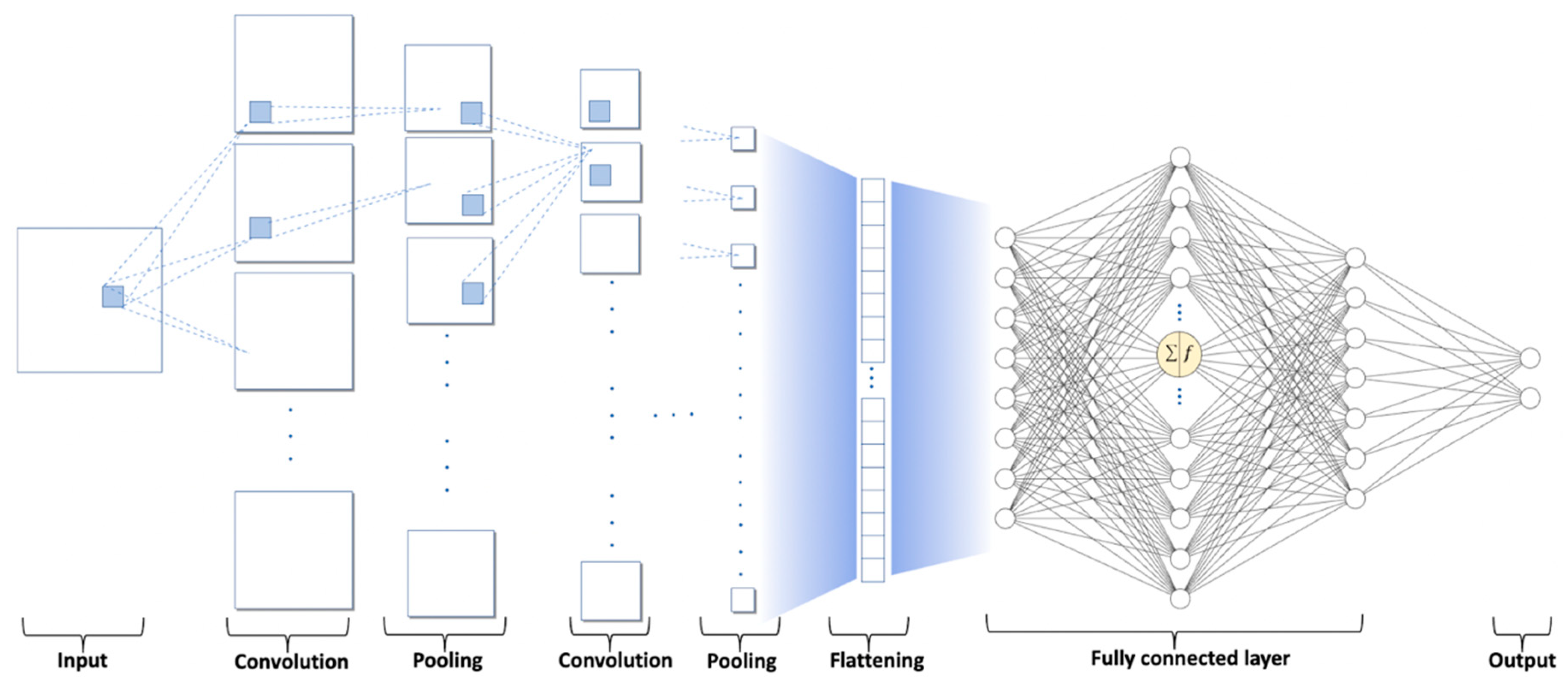
3.1. Brief Review of CNNs

The following section briefly explains a vanilla convolutional neural network. Figure 4 illustrates the basic components of a CNN model. The objective is to develop a model capable of recognizing tasks from pipeline images.

Input layer: This kind of architecture can input grayscale or multi-band images. A digital grayscale image can be seen as a grid of pixels with different brightness intensities. The computer interprets this grid of pixels as a 2D tensor with pixel values ranging from 0 for the darker pixels to 255 for the brighter pixels. Contrary to a multi-layer perceptron, in which the input matrix must be transformed into a 1D vector to go to the next step, a CNN accepts matrices and spatial context. Input data are normalized for faster learning convergence and better generalization. Moreover, all pictures must be reshaped to have the same height and width to feed the convolutional neural network.

Convolutional layer and pooling layer: The first part of the convolutional neural network is composed of convolution and pooling layers. The image passes through multiple convolutional and pooling layers to detect patterns and extract features called feature maps. A feature can be seen as a datum in an image that distinguishes one object from another. Meaningful features are extracted thanks to a convolutional layer that can be seen as a sliding window (a convolutional filter) which performs the convolution with the image pixel by pixel. A modified image with new pixel values is then obtained. After that, pooling layers can be applied to reduce the computational complexity and keep important features [41].

Flattening layer: The extracted features must be put into the multi-layer perceptron for classification tasks. However, a multi-layer perceptron only takes 1D tensors as input. Therefore, a flattening layer is used to convert the feature map’s tensor into this adapted format.

Output: From the multi-layer perceptron, the classification task can be performed using the features extracted from the picture. Finally, with a classification problem, the fully connected layers return probability values for each class.

Figure 4 illustrates how CNN models process a picture to extract useful information (features) and perform a required task (classification, regression, segmentation, etc.). Nevertheless, before having this ability, the model must be trained. During the training phase, the parameters (weights) of the different layers of the CNN model are optimized to perform a specific task. This optimization is performed iteratively using a backpropagation gradient algorithm. In the case of supervised learning, the model prediction is compared to the ground truth. Finally, an error function (loss function) between the predicted and ground truth label is computed. The model weights are adjusted consequently to reduce the loss function value. Among CNN algorithms for object detection [42], the “You Only Look Once” (YOLO) family has different versions. YOLOV7 is one of the state-of-the-art object detection models in the YOLO series [43,44,45,46,47]. There are different versions of the YOLO algorithm; however, controversies are present in the computer community. In fact, YOLOV1 to YOLOV4 are considered as official YOLO models, but some researchers or companies have published YOLOV5 or YOLOV6 models, which are unofficial versions. The last official YOLO model is YOLOV7 (finally considered as the official YOLOV5). Compared with other object detection models, it demonstrates notable performance with its high detection accuracy, real-time monitoring ability, and model complexity [48,49,50,51,52]. In this study, the YOLOV7 model is used to detect the localization and size of oxygen bubbles in the PEMWE.

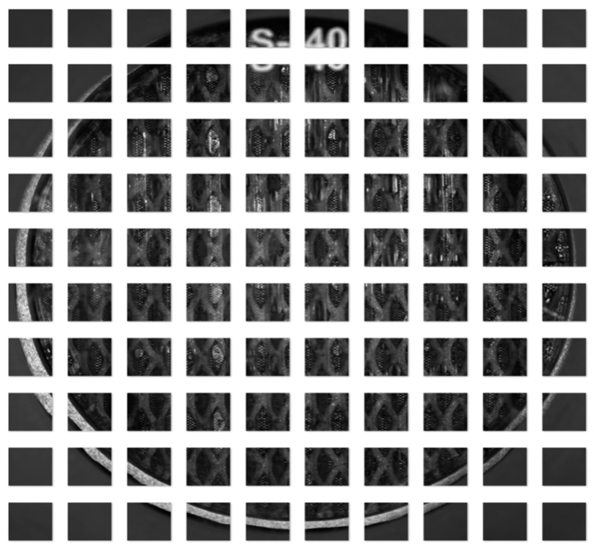
3.2. Dataset Preparation and Preprocessing

The dataset consists of images of the anodic oxygen bubbles of the PEMWE obtained using the high-density and high-frequency camera and two flashes to increase the illumination. The database consists of approximately 27,000 images in PNG format with a resolution of 5120 × 5120 pixels. The images were recorded at 65 FPS for about 20 s for different current and flow rate values of deionized water. First, they were recorded for a constant flow rate set to 0.4 L/min and with a current value ranging from 0.3 to 1.4 A/cm². Then, they were recorded for a constant current set to 1.4 A/cm² with a flow rate value ranging from 0.05 L/min to 0.40 L/min. The anodic and cathodic temperatures are regulated to 60 °C, and the cathodic and anodic pressures are set to 1 atm. After modifying an operating parameter (e.g., the current or water flow), the camera recording was only activated when the stable operating state of the PEMWE was reached. Each experiment produced approximately 400 Go of data. A polarization curve of the system is given in Figure 5.

In order to train the model, a labeled dataset is required in supervised learning. LabelImgtool is written in Python and is a graphical image annotation tool by Tzutalin [53], available on GitHub. It is used to create annotations, which consists of manually identifying and locating all bubbles in a frame. Then, a saved file with the positions of all the annotations in the picture is created. To be efficient, the training phase requires a sufficient amount of data. Therefore, labeling is still the most time-consuming step to obtain a workable dataset. In order to preserve the high resolution for small bubbles, a slicing operation of the high-resolution image into about 100 thumbnails is chosen, as illustrated in Figure 6.

The model is designed to accept 512 × 512 pixel images as input. With this sliding preprocessing, since some bubbles may be cut between two thumbnails, some bubbles may not be labeled entirely. Nevertheless, the main information (bubble recognition, identification, and localization) is globally saved. It is essential to note that the labeled dataset must be divided into three sub-datasets to perform all the learning steps: the training, testing, and validation sets. For this study, the previous three sub-datasets represent 80%, 10%, and 10% of the labeled image database, respectively.

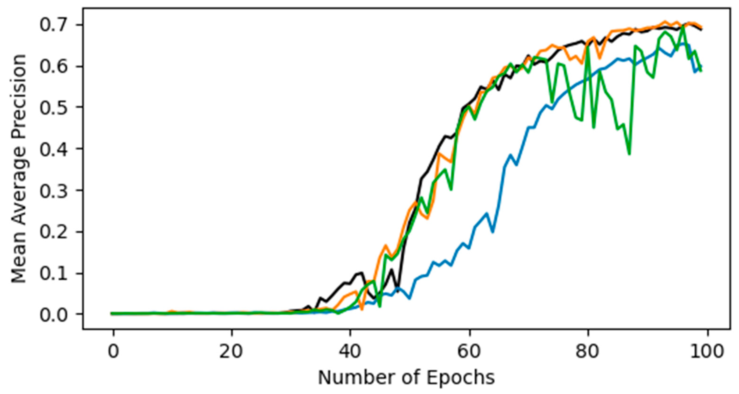
3.3. Training, Inference, and Post-Processing

The training step is performed with Python frameworks, and libraries such as Tensorflow or OpenCV are used. The GPU of the computer is used to speed up the calculations.

After specifying the different basic parameters of the standard architecture of YOLOV7, such as the number of epochs, image size, batch size, or the pathway of the training dataset, the YOLOV7 algorithm can be trained. It is worth noting that more than 30 other hyperparameters exist, and their values can be optimized to improve the training step. However, in this study, the vast majority of default values were kept constant.

Table 1. Some customizable hyperparameters, excluding image input size and batch size, which are all default values.

Image Input Size: 512	Momentum: 0.937
Batch size: 4	Weight-decay: 0.0005
Learning-rate start (lr0): 0.01	Conf threshold: 0.25

shows some of them.

It is important to highlight that to reduce the amount of data required to train the model, a pre-trained YOLOV7 model is used, and only the last layer (the classification layer) is (re)trained. All other parameters (weights) remain unchanged and are frozen during the training phase. Note that the YOLOV7 model has been pre-trained using the MS COCO dataset (328,000 pictures and 80 classes). After the training step, an output file called the weight file is obtained. This file contains information about the different weight values required to perform bubble detection. To perform detection on new images, the weight file path must be specified in the script. After that, new images can be used as input for the YOLOV7 architecture to perform detection. The model is designed to use a 512 × 512 pixel picture size, so the inference step requires the same picture size. For this reason, all pictures in the dataset are also split into one hundred thumbnails. Then, the detection occurs in these 512 × 512 pictures. It should be noted that slicing before detecting increases the detection time. Afterward, the neural network architecture produces a results file for each thumbnail. A post-processing step was performed with the result files mentioned above to extract essential information, such as the number of detected bubbles and their position. The detected bubbles are in rectangular boxes, like in the labeling step. With the box coordinate, the box area can be calculated. However, it is far from the natural bubble surface situated in the box. Therefore, a ratio is calculated to be more realistic when estimating bubble coverage. In the PEMWE, there are different bubble sizes, which is why the detection boxes also have different sizes. Bubbles of different sizes with their associated boxes were selected to calculate the ratio. To obtain the correct ratio, the number of pixels occupied by the bubble in the picture is divided by the number of pixels occupied by its detection box. A ratio of 0.7 is obtained; in other words, 70% of the pixels contained in a detection box represent the bubble. Therefore, to estimate the bubble coverage over the whole anodic side of the PEMWE, all box areas are calculated, and then the ratio is applied.

4. Experimental Results

This section presents the results obtained after the inference and post-processing steps of the 27,000 images. In this study, the bubble coverage takes into account all the bubbles present between the liquid gas diffusion layer interface and the channels. Most of them are bubbles that remain attached due to the surface tension force until the dynamic pressure of the flowing water becomes greater than the surface tension force. Then they detach and are evacuated. The mean bubble area is obtained by adding all the area occupied by bubbles over the liquid gas diffusion layer in an image, divided by the amount of bubbles present in the same image. Thus, the average size of the bubbles present in the picture is obtained. As each value of the water flow rate or current density represent around 1300 images (20 s), the bubble coverage, number of bubbles, and mean bubble area are computed 1300 times. Then the average values of these 1300 results are calculated, and one box plot can be represented. According to the literature, these three parameters are influenced by the water flow rate, which can increase the frequency of bubble detachment, or by the current density, which acts on the bubble size detachment process [54].

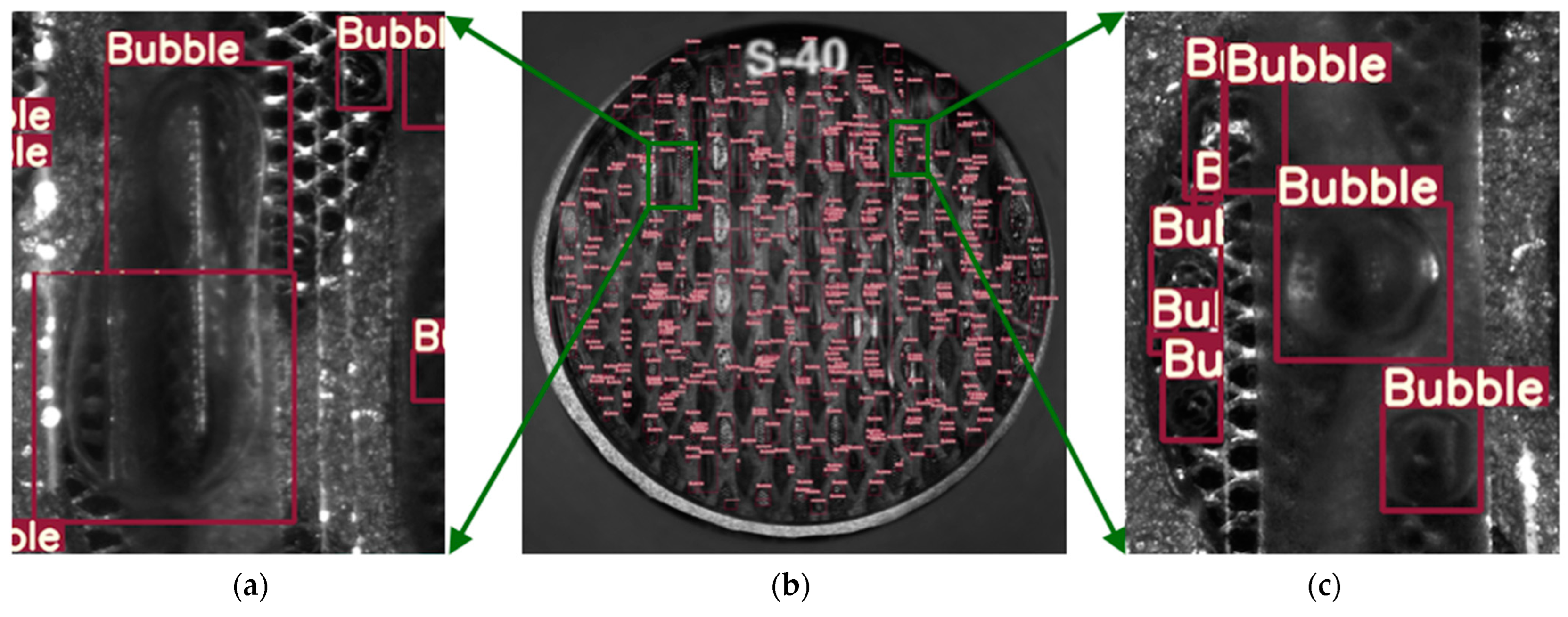
4.1. Inference Results

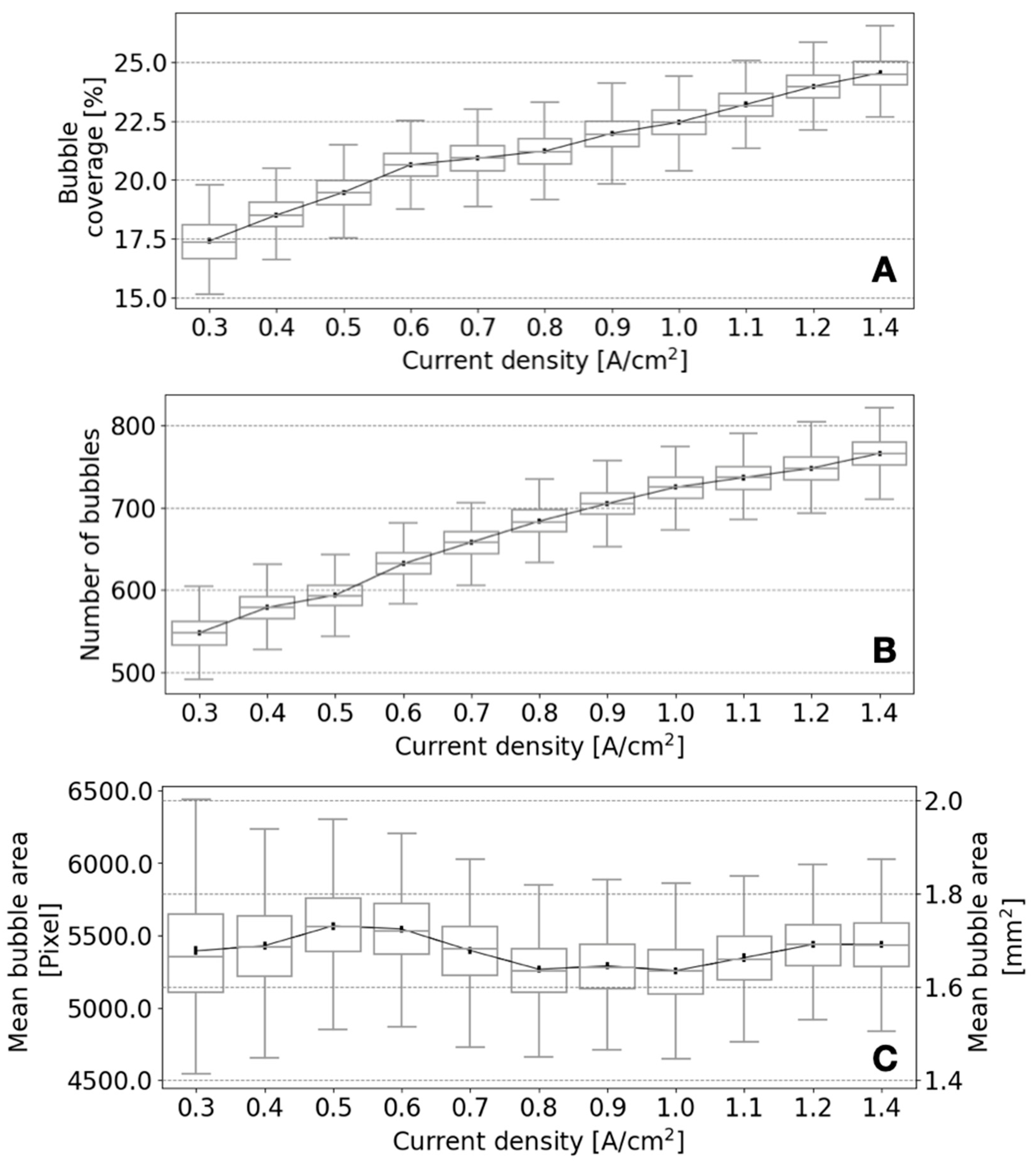
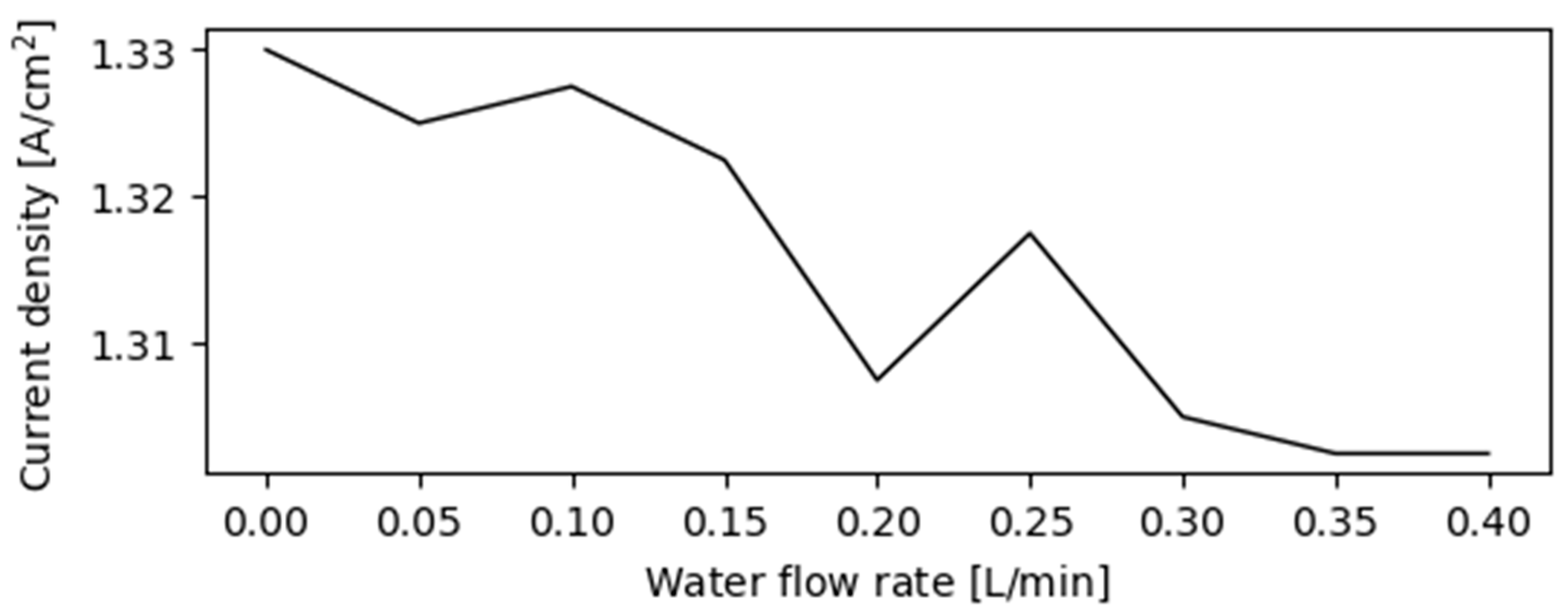
Figure 7 analyzes the bubble flow’s evolution following the variation in water input flow. The output of the YOLOV7 model is post-processed to obtain the following: the anodic bubble coverage (Figure 7A), the number of bubbles over the anodic side (Figure 7B), and the individual mean surface of the bubbles (Figure 7C). In Figure 7A, the bubble coverage decreases when the water flow rate increases by around 32%. Su et al. [22] obtained the same behavior with their simulation. When the water flow rate increases, it facilitates the evacuation of bubbles and detachment from the electrode surface area due to the higher flow drag force. If the bubble detachment frequency increases, the number of bubbles may increase greatly. However, the increase in the bubbles’ evacuation ability created by a higher water flow rate leads to a counterbalance. The number of bubbles increases slightly, as seen in Figure 7B. Moreover, a faster bubble detachment frequency leads to a decrease in the bubble detachment diameter, as mentioned by Li et al. [24]. This is what can be deduced from Figure 7C, which shows a decrease in the mean bubble area when the water flow rate increases. It is also in concordance with the observation made by Dedigama et al. [19] in their paper.

Figure 8 analyzes the evolution of bubble flow following the variation in the current density. The results show that the bubble coverage increase by around 40% when current density increase. And the number of bubbles increase too when current density increase. This behavior is in agreement with the optical visualization allowed by the transparent cell, which is what Su et al. [22] deduced in their simulation as well as other authors in the literature, such as Li et al. [24]. The second Faraday law explains this phenomenon physically. If the amount of electricity increases, the amount of oxygen and number of reaction sites also increase. Moreover, as Li et al. [24] and Su et al. [22] mentioned, the bubble detachment diameter will also increase. However, this is not the case in our study, as depicted in Figure 8C, which gives an idea about the general bubble size in the PEMWE. This graph appears to have bigger bubbles at around 0.5 A/cm² and smaller ones at 1 A/cm². Nevertheless, it should be essential to go deeper to better understand this graph behavior before interpreting it. Some stagnant bubbles are present among conventional bubbles. The size of stagnant bubbles could have a non-negligible influence over the curve trend.

4.2. Discussion

One common way to evaluate a CNN model’s performance in detection after training is to examine the mean average precision (mAP) curve. For this study, four training rounds have been performed with different seeds (which control the weight initialization values) and the best train results in a mAP around 70%, as shown in Figure 9, the orange-colored curve, before stabilization. However, a better mAP could be obtained if the hyper-parameters are optimized.

In the literature, from one author to another, the effect of the water flow rate on the electrochemical performance differs. Some of them found that when it increases, the performance decreases (Dedigama et al. [10]), while others have found the opposite (Su et al. [22]). With the deep learning approach, as the bubble coverage decreases when the water flow rate increases, it initially looks as if the performance may increase due to the better evacuation. However, during our experiments, for a fixed voltage, the current density of the PEMWE decreased when the water flow rate increased (Figure 10). The tool is not yet able to link the decreasing performance (showed by the decreasing current density) and the oxygen bubbles’ behavior to understand and clarify this question. This is why an improved version of this tool is so necessary.

Figure 11b shows the result obtained for one picture after detection with YOLOV7. Since inference appears on the thumbnails, all the thumbnails are reassembled to obtain the image shown in Figure 11b. Detected bubbles are represented by red rectangular frames as seen in Figure 11a,c, which are zoomed-in images of two small parts (the green rectangles) of Figure 11b. Moreover, the large bubbles are framed by several red rectangles, which increases the error in identifying the number of bubbles or the bubble rate coverage on the surface medium. This is why the detection is performed on thumbnail images, and the large bubbles are divided into several thumbnail images. Therefore, the algorithm cannot observe the bubble entirely. Typically, this problem occurs when a bubble is involved in more than two thumbnails. One approach to partially solve this problem would be to develop an algorithm that can overlap thumbnails to capture a more significant portion of the large bubbles. However, this approach would again increase the detection time, and real-time applications may not be possible. Moreover, as shown in the previous section, stagnant bubbles could have a significant influence on the results, which is why multi-label detection is necessary to differentiate them.

In the detection result, some false bubble detections can be observed. Indeed, some red rectangles do not enclose any bubbles, which leads to an increase in the error associated with the estimation of the coverage and the number of bubbles. This problem could be solved by considering an additional post-processing step. Moreover, this step would allow for the fusion of identical bubbles that are present side by side. However, this would significantly negatively impact the algorithm’s speed, which prevents real-time applications.

Moreover, through visualization, a non-uniform flow pattern is observed, induced by the position of the water inlet and outlet located at the lower left and upper right of the PEMWE. It is noted that there are no stagnant bubbles at the channels’ output, as observed by Maier et al. [21] with the topology of the PEMWE they used. Lastly, the algorithm can see more bubbles compared to those detected by hand labeling. In other words, many tiny bubbles could be missed during the labeling process due to a lack of human vigilance. Hence, as the model performance is evaluated, compared to that of labeled images, the real mAP may be up to 70%. Despite our promising results, as discussed, some improvements can be made for more precise and detailed results.

5. Conclusions and Prospect

In this paper, for the first time, a deep-learning-based bubble flow recognition tool dedicated to PEM water electrolyzers was developed. The performance of the proposed tool was experimentally evaluated on a real PEMWE system. The first results were very promising and showed that bubble information in a PEMWE can be successfully extracted. The state-of-the-art YOLOV7 architecture was chosen as the most suitable for this study. It was shown that the proposed CNN model could effectively detect anodic bubbles in a PEMWE with a mean average precision of 70%. The obtained results were analyzed and concurred with the experimental visualization and different studies from the literature. When current density increases, the anodic bubble coverage and bubble number increase. However, further experiments need to be performed to interpret the bubbles and extract more information from the mean size curve. The literature mentions that the mean bubble area decreases when the anodic water flow rate increases. Nonetheless, it has been hypothesized that the water speed and coalescence coupling effect between bubbles should explain why the number of bubbles remains the same. Further studies must be conducted to verify this explanation. Further works are in progress to develop an algorithm that can overlap vignettes to capture a more significant portion of large bubbles. In addition, for the better discretization of bubble regimes in PEMWEs, it is necessary to distinguish different classes of bubbles. Bubble tracking is also part of our outlook. We will analyze other configurations of the electrolyzer with the developed tool. This will provide more information about the influence of different components of the PEMWE over the bubbles. Moreover, the water flow rate and current density are not the only parameters that influence bubble characteristics. Indeed, higher temperatures, which can enhance upward gas transport [54], or even the pressure in the PEMWE have an impact on bubbles. Due to the fact that this is the first time a CNN approach has been used for bubble detection in a PEMWE and, more generally, the first time that curves have been obtained from experimental data, these results cannot yet be compared with those of other approaches in the literature. Moreover, great attention must be paid when comparisons must be made due to the fact that some parameters (the grid topology, current density, water flow rate, the cell shape, membrane, dimensions, etc.) are not the same from one PEMWE to another.

References

1. Dawood, F.; Anda, M.; Shafiullah, G.M. Hydrogen Production for Energy: An Overview. Int. J. Hydrogen Energy 2020, 45, 3847–3869. [Google Scholar] [CrossRef]
2. K/bidi, F.; Damour, C.; Grondin, D.; Hilairet, M.; Benne, M. Multistage Power and Energy Management Strategy for Hybrid Microgrid with Photovoltaic Production and Hydrogen Storage. Appl. Energy 2022, 323, 119549. [Google Scholar] [CrossRef]
3. Johnson, S.C.; Rhodes, J.D.; Webber, M.E. Understanding the Impact of Non-Synchronous Wind and Solar Generation on Grid Stability and Identifying Mitigation Pathways. Appl. Energy 2020, 262, 114492. [Google Scholar] [CrossRef]
4. Al-Shetwi, A.Q.; Hannan, M.A.; Jern, K.P.; Mansur, M.; Mahlia, T.M.I. Grid-Connected Renewable Energy Sources: Review of the Recent Integration Requirements and Control Methods. J. Clean. Prod. 2020, 253, 119831. [Google Scholar] [CrossRef]
5. Kovač, A.; Paranos, M.; Marciuš, D. Hydrogen in Energy Transition: A Review. Int. J. Hydrogen Energy 2021, 46, 10016–10035. [Google Scholar] [CrossRef]
6. Ishaq, H.; Dincer, I.; Crawford, C. A Review on Hydrogen Production and Utilization: Challenges and Opportunities. Int. J. Hydrogen Energy 2022, 47, 26238–26264. [Google Scholar] [CrossRef]
7. Carmo, M.; Fritz, D.L.; Mergel, J.; Stolten, D. A Comprehensive Review on PEM Water Electrolysis. Int. J. Hydrogen Energy 2013, 38, 4901–4934. [Google Scholar] [CrossRef]
8. Maier, M.; Smith, K.; Dodwell, J.; Hinds, G.; Shearing, P.R.; Brett, D.J.L. Mass Transport in PEM Water Electrolysers: A Review. Int. J. Hydrogen Energy 2022, 47, 30–56. [Google Scholar] [CrossRef]
9. Falcão, D.S.; Pinto, A.M.F.R. A Review on PEM Electrolyzer Modelling: Guidelines for Beginners. J. Clean. Prod. 2020, 261, 121184. [Google Scholar] [CrossRef]
10. Dedigama, I.; Angeli, P.; Ayers, K.; Robinson, J.B.; Shearing, P.R.; Tsaoulidis, D.; Brett, D.J.L. In Situ Diagnostic Techniques for Characterisation of Polymer Electrolyte Membrane Water Electrolysers—Flow Visualisation and Electrochemical Impedance Spectroscopy. Int. J. Hydrogen Energy 2014, 39, 4468–4482. [Google Scholar] [CrossRef]
11. Ito, H.; Maeda, T.; Nakano, A.; Takenaka, H. Properties of Nafion Membranes under PEM Water Electrolysis Conditions. Int. J. Hydrogen Energy 2011, 36, 10527–10540. [Google Scholar] [CrossRef]
12. Nie, J.; Chen, Y.; Cohen, S.; Carter, B.D.; Boehm, R.F. Numerical and Experimental Study of Three-Dimensional Fluid Flow in the Bipolar Plate of a PEM Electrolysis Cell. Int. J. Therm. Sci. 2009, 48, 1914–1922. [Google Scholar] [CrossRef]
13. Selamet, O.F.; Pasaogullari, U.; Spernjak, D.; Hussey, D.S.; Jacobson, D.L.; Mat, M.D. Two-Phase Flow in a Proton Exchange Membrane Electrolyzer Visualized in Situ by Simultaneous Neutron Radiography and Optical Imaging. Int. J. Hydrogen Energy 2013, 38, 5823–5835. [Google Scholar] [CrossRef]
14. Aubras, F.; Deseure, J.; Kadjo, J.-J.A.; Dedigama, I.; Majasan, J.; Grondin-Perez, B.; Chabriat, J.-P.; Brett, D.J.L. Two-Dimensional Model of Low-Pressure PEM Electrolyser: Two-Phase Flow Regime, Electrochemical Modelling and Experimental Validation. Int. J. Hydrogen Energy 2017, 42, 26203–26216. [Google Scholar] [CrossRef]
15. Majasan, J.O.; Cho, J.I.S.; Dedigama, I.; Tsaoulidis, D.; Shearing, P.; Brett, D.J.L. Two-Phase Flow Behaviour and Performance of Polymer Electrolyte Membrane Electrolysers: Electrochemical and Optical Characterisation. Int. J. Hydrogen Energy 2018, 43, 15659–15672. [Google Scholar] [CrossRef]
16. Hoeh, M.A.; Arlt, T.; Kardjilov, N.; Manke, I.; Banhart, J.; Fritz, D.L.; Ehlert, J.; Lüke, W.; Lehnert, W. In-Operando Neutron Radiography Studies of Polymer Electrolyte Membrane Water Electrolyzers. ECS Trans. 2015, 69, 1135–1140. [Google Scholar] [CrossRef]
17. Ito, H.; Maeda, T.; Nakano, A.; Hasegawa, Y.; Yokoi, N.; Hwang, C.M.; Ishida, M.; Kato, A.; Yoshida, T. Effect of Flow Regime of Circulating Water on a Proton Exchange Membrane Electrolyzer. Int. J. Hydrogen Energy 2010, 35, 9550–9560. [Google Scholar] [CrossRef]
18. Sadeghi Lafmejani, S.; Olesen, A.C.; Al Shakhshir, S.; Kær, S.K. Analysing Gas-Liquid Flow in PEM Electrolyser Micro-Channels Using a Micro-Porous Ceramic as Gas Permeable Wall. ECS Trans. 2017, 80, 1107–1115. [Google Scholar] [CrossRef]
19. Dedigama, I.; Angeli, P.; van Dijk, N.; Millichamp, J.; Tsaoulidis, D.; Shearing, P.R.; Brett, D.J.L. Current Density Mapping and Optical Flow Visualisation of a Polymer Electrolyte Membrane Water Electrolyser. J. Power Sources 2014, 265, 97–103. [Google Scholar] [CrossRef]
20. Maier, M.; Meyer, Q.; Majasan, J.; Tan, C.; Dedigama, I.; Robinson, J.; Dodwell, J.; Wu, Y.; Castanheira, L.; Hinds, G.; et al. Operando Flow Regime Diagnosis Using Acoustic Emission in a Polymer Electrolyte Membrane Water Electrolyser. J. Power Sources 2019, 424, 138–149. [Google Scholar] [CrossRef]
21. Maier, M.; Meyer, Q.; Majasan, J.; Owen, R.E.; Robinson, J.B.; Dodwell, J.; Wu, Y.; Castanheira, L.; Hinds, G.; Shearing, P.R.; et al. Diagnosing Stagnant Gas Bubbles in a Polymer Electrolyte Membrane Water Electrolyser Using Acoustic Emission. Front. Energy Res. 2020, 8, 582919. [Google Scholar] [CrossRef]
22. Su, X.; Xu, L.; Hu, B. Simulation of Proton Exchange Membrane Electrolyzer: Influence of Bubble Covering. Int. J. Hydrogen Energy 2022, 47, 20027–20039. [Google Scholar] [CrossRef]
23. Garcia-Navarro, J.C.; Schulze, M.; Friedrich, K.A. Detecting and Modeling Oxygen Bubble Evolution and Detachment in Proton Exchange Membrane Water Electrolyzers. Int. J. Hydrogen Energy 2019, 44, 27190–27203. [Google Scholar] [CrossRef]
24. Li, Y.; Yang, G.; Yu, S.; Mo, J.; Li, K.; Xie, Z.; Ding, L.; Wang, W.; Zhang, F.-Y. High-Speed Characterization of Two-Phase Flow and Bubble Dynamics in Titanium Felt Porous Media for Hydrogen Production. Electrochim. Acta 2021, 370, 137751. [Google Scholar] [CrossRef]
25. Ilonen, J.; Juránek, R.; Eerola, T.; Lensu, L.; Dubská, M.; Zemčík, P.; Kälviäinen, H. Comparison of Bubble Detectors and Size Distribution Estimators. Pattern Recognit. Lett. 2018, 101, 60–66. [Google Scholar] [CrossRef]
26. Nielsen, F. Detecting Lines in Images: The Hough Transform; Sony Computer Science Laboratories, Inc.: Tokyo, Japan, 2011. [Google Scholar] [CrossRef]
27. Ayala-Ramirez, V.; Garcia-Capulin, C.H.; Perez-Garcia, A.; Sanchez-Yanez, R.E. Circle Detection on Images Using Genetic Algorithms. Pattern Recognit. Lett. 2006, 27, 652–657. [Google Scholar] [CrossRef]
28. Pan, L.; Chu, W.-S.; Saragih, J.M.; De la Torre, F.; Xie, M. Fast and Robust Circular Object Detection With Probabilistic Pairwise Voting. IEEE Signal Process. Lett. 2011, 18, 639–642. [Google Scholar] [CrossRef]
29. Taboada, B.; Vega-Alvarado, L.; Córdova-Aguilar, M.S.; Galindo, E.; Corkidi, G. Semi-Automatic Image Analysis Methodology for the Segmentation of Bubbles and Drops in Complex Dispersions Occurring in Bioreactors. Exp. Fluids 2006, 41, 383–392. [Google Scholar] [CrossRef]
30. Viola, P.; Jones, M. Rapid Object Detection Using a Boosted Cascade of Simple Features. In Proceedings of the 2001 IEEE Computer Society Conference on Computer Vision and Pattern Recognition. CVPR 2001, Kauai, HI, USA, 8–14 December 2001; Volume 1, pp. I-511–I-518. [Google Scholar] [CrossRef]
31. Dalal, N.; Triggs, B. Histograms of Oriented Gradients for Human Detection. In Proceedings of the 2005 IEEE Computer Society Conference on Computer Vision and Pattern Recognition (CVPR’05), San Diego, CA, USA, 20–25 June 2005; Volume 1, pp. 886–893. [Google Scholar] [CrossRef]
32. Poletaev, I. Bubble Patterns Recognition Using Neural Networks: Application to the Analysis of a Two-Phase Bubbly Jet. Int. J. Multiph. Flow 2020, 14, 103194. [Google Scholar] [CrossRef]
33. Wang, Q.; Li, X.; Xu, C.; Yan, T.; Li, Y. Bubble Recognizing and Tracking in a Plate Heat Exchanger by Using Image Processing and Convolutional Neural Network. Int. J. Multiph. Flow 2021, 138, 103593. [Google Scholar] [CrossRef]
34. Park, H.; Choi, D.; Kim, H. Bubble Velocimetry Using the Conventional and CNN-Based Optical Flow Algorithms. Sci. Rep. 2022, 12, 11879. [Google Scholar] [CrossRef]
35. Cui, Y.; Li, C.; Zhang, W.; Ning, X.; Shi, X.; Gao, J.; Lan, X. A Deep Learning-Based Image Processing Method for Bubble Detection, Segmentation, and Shape Reconstruction in High Gas Holdup Sub-Millimeter Bubbly Flows. Chem. Eng. J. 2022, 449, 137859. [Google Scholar] [CrossRef]
36. Xiang, Z.; Xie, B.; Fu, R.; Qian, M. Advanced Deep Learning-Based Bubbly Flow Image Generator under Different Superficial Gas Velocities. Ind. Eng. Chem. Res. 2022, 61, 1531–1543. [Google Scholar] [CrossRef]
37. Kim, Y.; Park, H. Deep Learning-Based Automated and Universal Bubble Detection and Mask Extraction in Complex Two-Phase Flows. Sci. Rep. 2021, 11, 8940. [Google Scholar] [CrossRef] [PubMed]
38. Cerqueira, R.F.L.; Paladino, E.E. Development of a Deep Learning-Based Image Processing Technique for Bubble Pattern Recognition and Shape Reconstruction in Dense Bubbly Flows. Chem. Eng. Sci. 2021, 230, 116163. [Google Scholar] [CrossRef]
39. Haas, T.; Schubert, C.; Eickhoff, M.; Pfeifer, H. BubCNN: Bubble Detection Using Faster RCNN and Shape Regression Network. Chem. Eng. Sci. 2020, 216, 115467. [Google Scholar] [CrossRef]
40. Gong, C.; Song, Y.; Huang, G.; Chen, W.; Yin, J.; Wang, D. BubDepth: A Neural Network Approach to Three-Dimensional Reconstruction of Bubble Geometry from Single-View Images. Int. J. Multiph. Flow 2022, 152, 104100. [Google Scholar] [CrossRef]
41. Chen, L.; Li, S.; Bai, Q.; Yang, J.; Jiang, S.; Miao, Y. Review of Image Classification Algorithms Based on Convolutional Neural Networks. Remote Sens. 2021, 13, 4712. [Google Scholar] [CrossRef]
42. Ren, J.; Wang, Y. Overview of Object Detection Algorithms Using Convolutional Neural Networks. J. Comput. Commun. 2022, 10, 115–132. [Google Scholar]
43. Wang, C.-Y.; Bochkovskiy, A.; Liao, H.-Y.M. YOLOv7: Trainable Bag-of-Freebies Sets New State-of-the-Art for Real-Time Object Detectors. arXiv 2022, arXiv:2207.02696. [Google Scholar]
44. Redmon, J.; Divvala, S.; Girshick, R.; Farhadi, A. You Only Look Once: Unified, Real-Time Object Detection. arXiv 2016, arXiv:1506.02640. [Google Scholar]
45. Redmon, J.; Farhadi, A. YOLO9000: Better, Faster, Stronger. arXiv 2016, arXiv:1612.08242. [Google Scholar]
46. Redmon, J.; Farhadi, A. YOLOv3: An Incremental Improvement. arXiv 2018, arXiv:1804.02767. [Google Scholar]
47. Bochkovskiy, A.; Wang, C.-Y.; Liao, H.-Y.M. YOLOv4: Optimal Speed and Accuracy of Object Detection. arXiv 2020, arXiv:2004.10934. [Google Scholar]
48. Pan, S.; Liu, J.; Chen, D. Research on License Plate Detection and Recognition System Based on YOLOv7 and LPRNet. AJST 2023, 4, 62–68. [Google Scholar] [CrossRef]
49. Wang, Y.; Wang, H.; Xin, Z. Efficient Detection Model of Steel Strip Surface Defects Based on YOLO-V7. IEEE Access 2022, 10, 133936–133944. [Google Scholar] [CrossRef]
50. Li, Y.; Lei, C.; Xue, Z.; Zheng, Z.; Long, Y. A Comparison of YOLO Family for Apple Detection and Counting in Orchards. Int. J. Comput. Syst. Eng. 2021, 15, 334–343. [Google Scholar]
51. Gillani, I.S.; Munawar, M.R.; Talha, M.; Azhar, S.; Mashkoor, Y.; Uddin, M.S.; Zafar, U. Yolov5, Yolo-x, Yolo-r, Yolov7 Performance Comparison: A Survey. In Artificial Intelligence and Fuzzy Logic System; Academy and Industry Research Collaboration Center (AIRCC): Chennai, India, 2022; pp. 17–28. [Google Scholar] [CrossRef]
52. Wu, D.; Jiang, S.; Zhao, E.; Liu, Y.; Zhu, H.; Wang, W.; Wang, R. Detection of Camellia Oleifera Fruit in Complex Scenes by Using YOLOv7 and Data Augmentation. Appl. Sci. 2022, 12, 11318. [Google Scholar] [CrossRef]
53. LabelImg. Available online: https://github.com/heartexlabs/labelImg (accessed on 26 March 2023).
54. Yuan, S.; Zhao, C.; Cai, X.; An, L.; Shen, S.; Yan, X.; Zhang, J. Bubble Evolution and Transport in PEM Water Electrolysis: Mechanism, Impact, and Management. Prog. Energy Combust. Sci. 2023, 96, 101075. [Google Scholar] [CrossRef]
Figure 1. (a) ETB; (b) visual acquisition systems.
Hydrogen 04 00036 g001
Figure 2. Expanded view of the circular anodic side of the PEMWE.
Hydrogen 04 00036 g002
Figure 3. View through anode window, in which darker parts with red dotted points are flow channels and hatched part is a rib (a); bubbles are observed in channels and under ribs (b).
Hydrogen 04 00036 g003
Figure 4. Basic convolutional neural network architecture.
Hydrogen 04 00036 g004
Figure 5. Polarization curve of the anode window of the PEMWE cell with anodic and cathodic water flow rate of 0.4 L/min, pressure of 1 atm, and water temperature of 60 °C.
Hydrogen 04 00036 g005
Figure 6. Thumbnails of the anodic part of the PEMWE.
Hydrogen 04 00036 g006
Figure 7. Evolution of bubble coverage (A); evolution of number of bubbles (B); evolution of mean bubble area compared to water flow rate (C).
Hydrogen 04 00036 g007
Figure 8. Evolution of bubble coverage (A); evolution of number of of bubbles (B); evolution in mean bubble area compared to current density (C).
Hydrogen 04 00036 g008
Figure 9. mAP curve variability with four different seeds. The orange curve is the one which reached the higher mAP at 100 epochs.
Hydrogen 04 00036 g009
Figure 10. Current density change when water flow rate increases.
Hydrogen 04 00036 g010
Figure 11. Detection results over the anodic part of PEMWE. (a,c) are zoomed-in images of the two green rectangles in (b).
Hydrogen 04 00036 g011