Blocking Hydrogen Diffusion in Palladium Cathode i—Analyzed by Electrochemistry; ii—Analyzed by Chaos

Abstract

Electrochemical chaos is caused when, during diffusion, hydrogen and, at worst, tritium is trapped in palladium after the formation of adsorbates. The mechanism leads to cracking corrosion, as seen by scanning electron microscopy. The instabilities were apprehended from voltammetry and electrochemical impedance spectroscopy in the active potential where the cathodic hydrogen is charged from two models of transients. Tests performed using an electrochemical chaos analyzer simplify the expertise of the palladium cathode in focusing on the blocking diffusion of hydrogen. A complex electrical circuit of chaos is considered for adsorption and the blocking diffusion. Depending on the active potential, distinct behavior such as the transformation of transients and limited diffusion can occur. Phase-space spectra are obtained, and synchronization has been developed to clarify the chaos leading to the cracking of palladium. By applying these different analytical tests for the restricted diffusion, it is possible to interpret the processes from the power spectra, autocorrelation function, or the divergence coefficient in the region of active potentials. Analyzers can detect flaws in this hydrogen diffusion process and suggest corrective measures.

1. Introduction

1.1. Hydrogen Interest

Before presenting the restricted diffusion and chaos, it is necessary to clarify hydrogen interest and how the hydrogen diffusion cathode works. Electrolysis by hydrogen charging the palladium responds to challenges replacing fossil fuels with clean energy. However, it is necessary, for an industrial electrolyzer producing hydrogen, that there is no leakage in the processing circuit towards the environment. To do this, engineers have to select a palladium alloy based on its resistance to stress corrosion cracking [1,2,3]. Unfortunately, finding a palladium alloy that exhibits a long life under these conditions is not easy. Palladium-silver diffusers are reliable in producing high purity hydrogen with high performance at high temperature and pose no difficulty for gas–gas diffusion [4,5,6]. How does the electrolyzer for the production of hydrogen isotopes work? Hydrogen adsorbs on the cathode surface during electrolysis, diffuses into the palladium, and is finally desorbed on the opposite side [7,8,9]. Desorption occurs in a gas-tight compartment separated from the electrolyzer to allow recovery of pure hydrogen without oxygen or moisture [10]. This work aims to provide a valuable contribution to estimate the resistance to cracking of the cathode [11], where water may contain hydrogen peroxide. Peroxide modifies the oxidizing power over a wide range of the active potential of palladium in the presence of adsorbed transients facilitating stress corrosion cracking [12,13]. Under these conditions, it is necessary to know the behavior of palladium charged in hydrogen from the reversible potential to the equilibrium potential [14,15,16]. In the present work, it is also a question of knowing the effects of these transients at alkaline pH on an unstable diffusion. This contribution will provide a detailed analysis of the blocking of hydrogen diffusion in the palladium cathode leading to chaos. Diffusion blocking is responsible for loss permeation. In this context, Figure 1 shows the electrolyzer for hydrogen production. To demonstrate blocking diffusion in this electrolyzer, it is necessary to localize where the blocking diffusion is produced using the chaos analyzer.

1.2. Electrochemistry and Chaos

For this, the present paper is organized into two parts, including the cyclic voltammetry and electrochemical impedance analysis; then, the chaos analysis obtained from our experimental results and their compilation data according to the following sections:

In Section 1.1, the results of the voltammetry curve for hydrogen adsorption are formulated;

In Section 1.2, the electrochemical impedance spectra in the active region for hydrogen adsorption are handled when diffusion is blocked in the thickness of the palladium membrane;

In Section 2, singular points of chaos in the active region from the reversible to the equilibrium potentials for hydrogen adsorption and blocking diffusion are clarified.

After presenting electrolysis by hydrogen charging on the diffusion cathode, the introduction should review recent publications to build an electrochemical chaos database. Then, a complex model will be used to make the experimental interpretation of diffusion blocking possible. These publications are the fruit of different sources going as far back as the year 2000, and some have been updated where possible. Results should provide the mechanisms in correlation with the chaos technique [17,18]. These previous reviews reported on the electrochemical chaos did not test the blocking diffusion. For this reason, this study was focused on our experimental results.

In the works [19,20], frequency relaxation depends on low-frequency electrochemical noise. Consequently, this noise can be determined from the behavior of electrode impedance. The measurements require converting the complex impedance signal into a data set to perform mathematical iterations with different approaches [21]. Then, the damaged surface was identified by micrography [22]. Results of examination revealed an inhomogeneous superficial structure. Therefore, the Nyquist spectra are helpful to diagnose the damage. Impedance modulus variation in low frequency indicates transitory steps. The equivalent circuit shows that the electrochemical noise follows the involved steps unambiguously.

In the study [23], a mathematical model is proposed by the equivalent electrical circuit. Results of the physical model show that the noise is influenced by the variation of the complex impedance at low frequency due to modification of the superficial structure of the metal.

Analysis of electrochemical noise impedance was also realized by Homborg [24,25]. When the low frequency is cut in sectors corresponding to each transient, the noise signal shows more detailed scrolls implying mechanisms. The analysis procedure involves the identification of transients in the electrochemical scrolls. These indicate the presence of successive steps representing transient activity ranging in the active potential. This procedure allows their identification.

According to [26], the electrochemical noise impedance provides the concept of complex diffusion. Based on these results, the correlation function was calculated by Grafov [27,28] using an electrochemical circuit implying a Warburg impedance. The noisy Warburg impedance in the circuit makes the system unstable. Moreover, its derivative characterizes the chronology of chaos. Therefore, the effect of Warburg impedance noise on the relaxation of transient has been established qualitatively.

Boffetta et al. [29] have documented chaos diffusion, giving dynamic steps. The concept of dynamical transients gives rise to different Lyapunov exponents. The correlation function and the divergence coefficient emphasize chaos. Impedance instabilities are observed in the electrochemical process, such as for local attacks, where the dynamic stress influences these. For that, Garcia et al. [30] have illustrated a relationship between constraint and chaos. Detailed diagnostics have been developed to characterize complex and irregular chronology corresponding to deterministic chaos rather than random noise. Chaotic disorders have been documented in the phase-space and from Lyapunov exponents. According to Yong-Jia Wei [31], the electrochemical noise indicates that the stress process can be divided into several steps featured by transients. Chaos analysis revealed the complexity of this system.

The electrochemical noise increases with increasing alkaline pH due to enhanced hydrogen adsorption and attack [32]. Electrochemical noise measurement makes it possible to detect the nucleation and growth of cracks [33]. When the palladium is not immunized against stress corrosion cracking, irregular signals are detected at low frequency. These signify metastable transients. In this case, the scroll series can be aperiodic. Dominant frequency in power spectra indicates the presence of the transient event. The electrochemical noise due to hydrogen was measured by Astafev [34,35].

Spiraling for the sorption of hydrogen in palladium has been described by Lalik [36], and equations have been formulated. On the basis of these, databases distinguish random or discrete divergence and convergence. The results applied to the aperiodic instability series suggest that the spiraling demonstrates the chaotic dynamic of hydrogen with the palladium. Considering the publication [37], the optical-electrochemical technique at high resolution makes it possible to visualize surface changes during the electrochemical noise. Correlation of these enables the identification of damaging processes in real-time, such as cracking in the subsurface. This visualization allows for analysis of the small sector of the exposed metal. This enables the quantification of the size, number, and nearest neighbor distance of local events, such as cracks. The optical analysis identifies electrochemical features sector by sector as a final result.

Besides these studies, Zhang et al. [38] have found that the local corrosion consists initially of metastable events. Qualitative analysis was applied for short sectors in frequency. The combination of sectors makes it possible to identify the mechanisms with high discrimination. Incorporating a fast Fourier transforms allows for determining the distribution of power frequency. Finally, they integrated the transient into the dominant frequency of the power spectra. In the case of multiple transients, each dominant frequency in the sequential is attributed to a transient. Therefore, monitoring the phase-space construction and fast Fourier transforms produce a methodology to obtain more extensive information on the nature of the attack [17,39]. Electrochemical chaos impedance spectroscopy is a powerful tool to explore heterogeneity. The factors limiting the resolution have been identified by MeiWenHuang [40]. This paper includes the interfacial and local impedance. Simulation shows that the impedance has typical behavior in the low frequency range.

Scanning electrochemical cell microscopy was deployed by [41] to study the electrochemical hydrogen absorption across the palladium. Cyclic voltammetry data reveal a dependence on the rate of hydrogen adsorption, absorption, and desorption across the active potential all in palladium oxide. Removing unwanted trends in impedance before calculating deviation and power spectral density is necessary, but the method is not always easy for electrochemical noise measurements. The procedure should be simple and not attenuate complex impedance acting at low frequency to avoid eliminating helptul information. Several procedures are presented by Bertocci [42], such as polynomial fitting and filtering. Their effects on the electrochemical signal are also discussed in applying different types of setups [43].

When the process is unstable, the signal exhibits a non-stationary state. An unbalanced signal has been identified as a transient. Analysis of electrochemical chaos signal appears to be a suitable method for obtaining information on the dynamic system, especially when scrolls are due to elementary events, as attraction or repulsion between charged transients. Therefore, this situation is encountered mainly in electrochemical processes with or without diffusion. By analyzing the scrolls and the rolling-up in phase-space, this technique provides qualitative analysis often inaccessible in the usual approach treating several signals in no steady-state.

It can be reported that electrochemical instability analysis is a valuable and powerful tool to study the fundamental aspect and for monitoring attacks [44]. Investigations indicate a considerable increase in interest in the behavior of nonlinear dynamical systems, as shown by J. Stringer A.J. Markworth [45]. Under some circumstances, these systems exhibit a behavior termed deterministic chaos. The complex behavior is extremely sensitive to the boundary conditions, and it is hardly predictable for an extended range of frequency. Different authors have developed many strategies. The limiting diffusion was observed by Grafov [46] using a Kramer function, allowing for dealing with several types of local diffusion. Under the condition of Gaussian electrochemical noise, the asymptotic Kramer function turns into a stochastic diffusion. Determining the homogeneous asymptotic Kramer function may be helpful to diagnose slow electrochemical hydrogen discharge and electrochemical noise. It is essential to study these dynamic aspects of chaos. Chaos for a dynamical and blocking system can be demonstrated using a data manipulation analyzer treating the voltammetry curves and electrochemical impedance spectra in interpolating the data to 2D or 3D format. Data analysis allows the plot of the phase–space diagrams and calculate the Lyapunov exponent [47]. The strategy is to acquire the data in dividing the global Lyapunov exponent into sectors to obtain the various predictability of the system for the restricted diffusion. Effectively, it is interesting to estimate the local predictability for a part of the phase-space. Local exponents are not invariant under blocking diffusion, and can represent several synchronized systems. They can be coupled such as a drive system and a subordinate system. The drive system is the one on which the relaxation of the chaotic signal depends. Synchronization occurs when all conditional exponents are negative or positive [48].

Blocking diffusion by charged hydrogen into palladium and propagation of stress corrosion cracks are shown in [17,49]. However, despite extensive research, no essential work in the literature was reported using a chaos analyzer when blocking diffusion is acting. The analyzer is suitable to bring out:

(a)

the exchange power between adsorbed hydrogen transients,

(b)

the divergence topology when diffusion is blocked.

Concretely, two regimes of diffusion will have to be examined:

(a)

subsurface diffusion,

(b)

diffusion over the thickness of palladium.

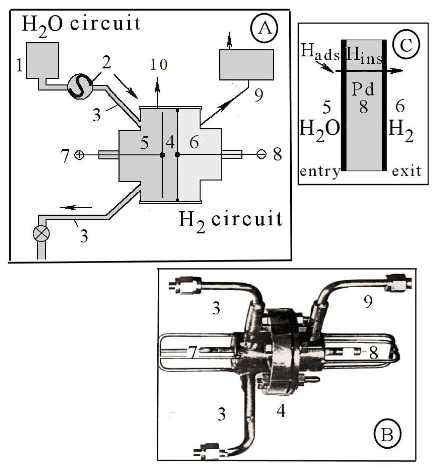
2. Methods and Materials

Previous work [11] showed that annealing treatment removes possible stress formed while cold rolling the palladium membrane. Stress has a significant effect on the diffusion phenomena. Stress release was not made before use because we wanted to investigate under the condition of limiting diffusion. Stressed palladium membranes cold rolled to 70 μm thick at high purity grade were supplied by the Comptoir Lyon Alemant Louyot company. To carry out our detailed analyses, the lateral side of the membrane was interlocked between two Teflon gaskets to avoid unwanted slight penetration of electrolyte between the palladium and the bearing causing random errors in the low-frequency range. Therefore, particular care was taken to make a suitable electrode for impedance and noise measurements.

Hydrogen formation depends on the applied potential. Consequently, the behavior of palladium was studied in the active region where hydrogen is produced using cyclic voltammetry, electrochemical impedance spectroscopy, and electrochemical noise analyzer. The electrochemical equipment consisted of a potentiostat and a triangular wave signal Radiometer Analytical generator connected to a digital Tektronix oscilloscope to show the transient formation in voltammetry at high scan. After storage in the oscilloscope, the digitized spectra were recorded on a Hewlett Packard plotter. An EIS Solartron analyzed the electrochemical impedance spectra. The reference and counter electrodes were, respectively, saturated calomel and platinum electrodes. A platinum wire was connected to the reference electrode through a 0.1 pF capacitor to eliminate any possible capacitive interference at low frequencies for impedance. The potentials are referred to as reversible hydrogen electrodes. The electrolyte was sodium hydroxide at pH 13. The temperature of the electrochemical cell was maintained constant at 20 °C. The spectra were obtained in potentiostatic mode, where the current is free to change. The measurement sequence was applied to a given potential that is stable to get the impedance spectrum with good reproducibility. The scans started at the highest frequency values, i.e., from 10³ Hz to 10⁻³ Hz, with a sinusoidal voltage amplitude of ±5 mV. The frequencies were scanned in a sequential mode step by step with ten steps per decade on a logarithmic scale. Two AC impedance measurements with Fourier transforms were carried out at each stage, and the spectra were judged to be satisfactory when they were identical over the low-frequency range. Then, the potential was shifted in a more positive direction to obtain a new impedance spectrum at this potential. Finally, the sequence was repeated from a defined potential range. The simulation was run on both the 2D and 3D data sets to interpret the experimental impedance spectra. Calculated values for the simulated model agree well with the experimental results. In particular, these produce identical Warburg impedances, making it possible to determine the diffusion parameters in the equivalent circuit between the observed spectra and the simulated fitting.

In the next operation, the SigmaPlot program interpolates the 3D data to obtain values in 2D mesh format to use them in the Chaos Data Analyzer program [50] to detect determinism. In 2D mesh format, projection represents the frequency and the impedance. An iterating number is imposed for the frequency giving the possibility to obtain chaotic entanglement motion for impedance. When chaos is found, calculation using the power spectrum, Lyapunov exponent, Eigenvalues, and autocorrelation and divergence functions enable the determination of qualitative and quantitative characteristics of the system. The program can be used sector by sector to make predictions on a singular local value. In these tests, electrochemical noise data are computed by a spectral method to lead to a phase-space portrait and understand the activity of palladium and diffusion organization. Finally, the TableCurve 2D program [51] was used to obtain the correlation function confirming the experimental conclusion.

The samples were examined with a Jeol scanning electron microscope to see embrittlement problems. Embrittlement results from blocking diffusion and leads to cracking.

i-Voltammogram and Impedance Spectra.

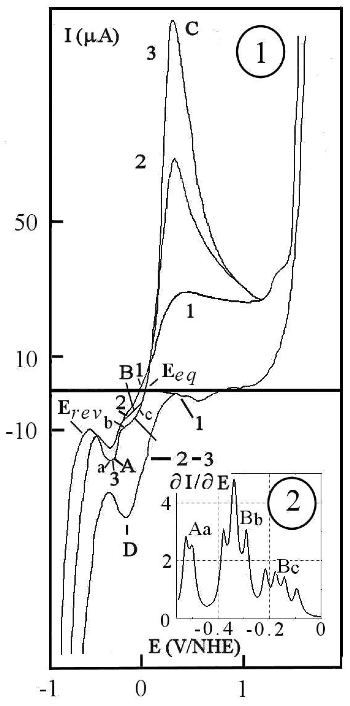
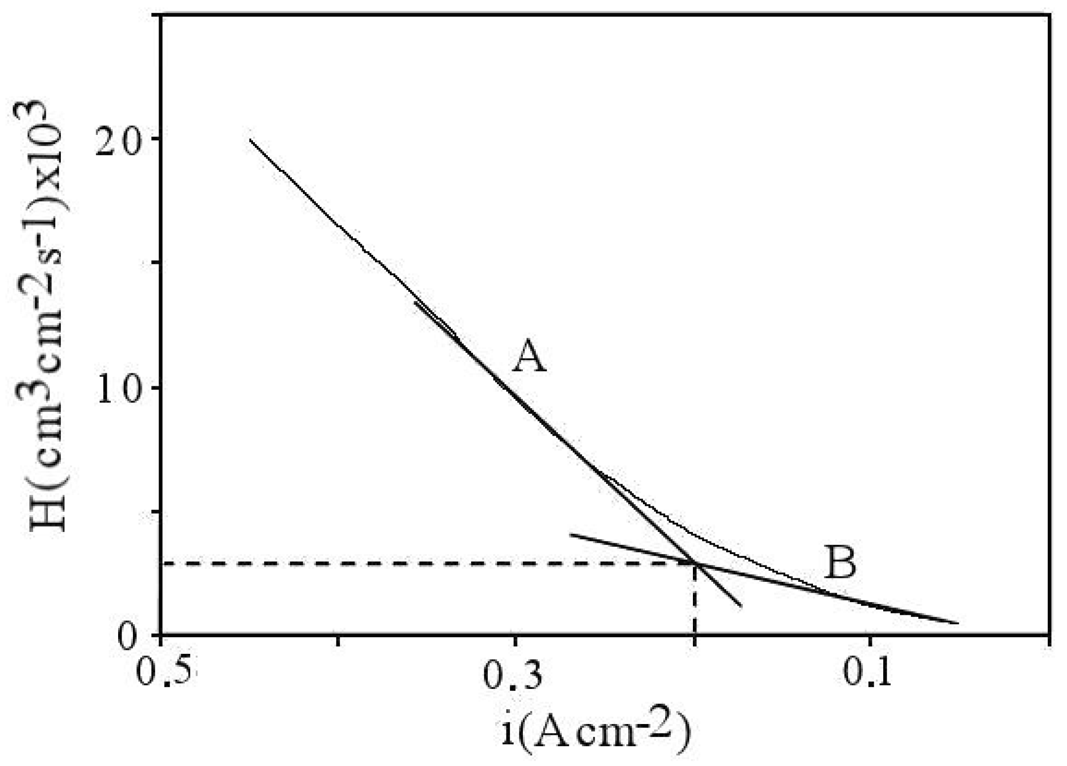
3. Scanning Voltammetry

Voltammetry is a powerful tool for exploring transients. For this, Figure 2(1) shows the voltammograms obtained on palladium cathode for a high sweep rate (v) and a time not too long for charging hydrogen to avoid a sizeable oxidizing current when back–diffusion of hydrogen occurs. The analyzed potentials will be between the reversibility and the equilibrium giving the complex shapes of the transient response for chaos. The presence of hydrogen peroxide allows for better viewing of adsorbed hydrogen peaks on the cathodic current. This was demonstrated using the radiolytic perhydroxyl in the tritium hydroxide. Moreover, incorporating hydrogen peroxide as an oxidant for biomass energy will create a new strategy and valorization of industrial hydrogen processes [52]. In this figure, the denomination is:

(A)

peak A for hydrogen adsorption on the forward scan,

(B)

shoulder B for the second hydrogen adsorption,

(C)

peak C for oxidation of back-diffused hydrogen and palladium,

(D)

peak D for hydrogen adsorption on the return scan.

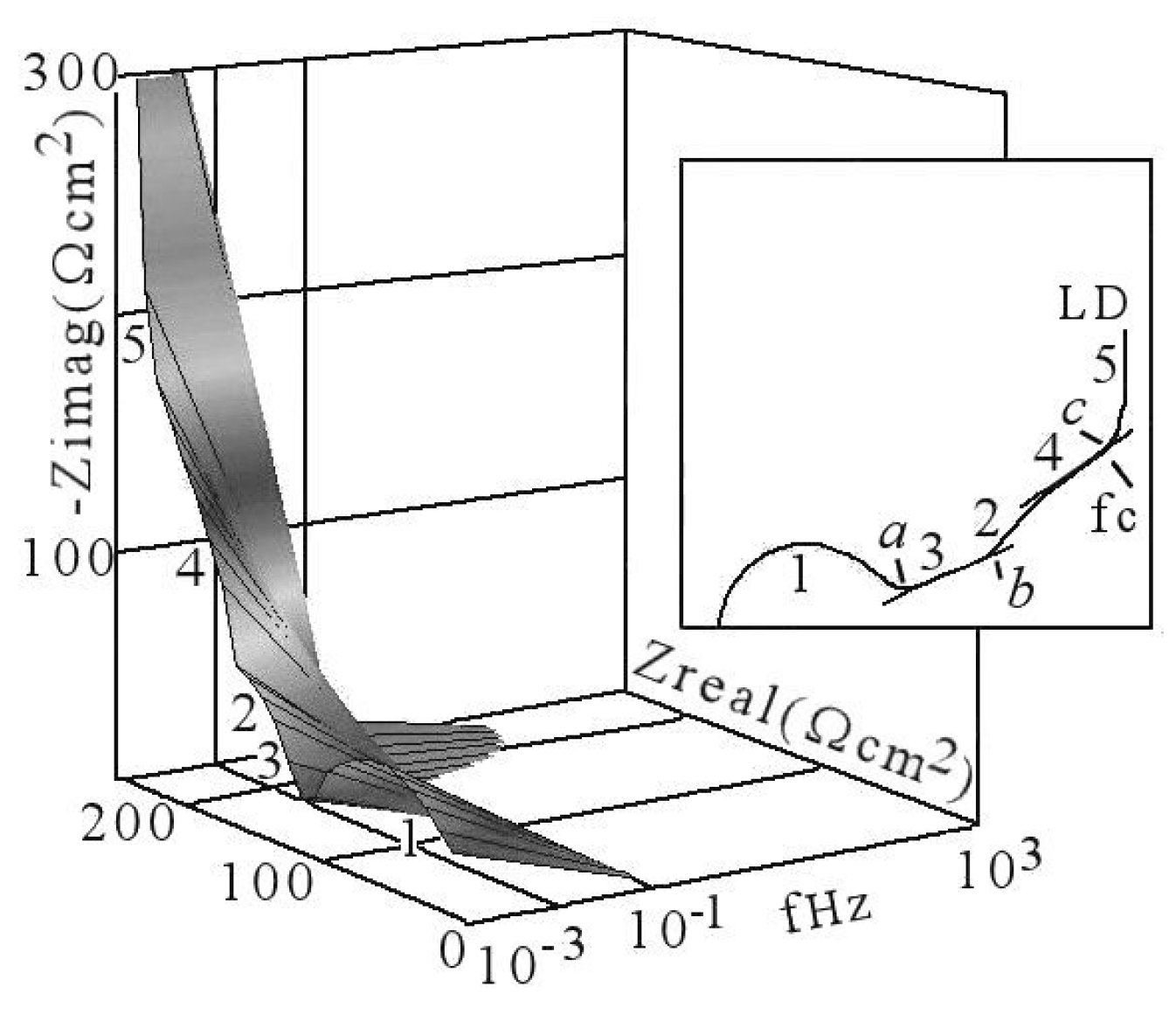
(a)

a on the peak A,

(b)

b between peak A and shoulder B,

(c)

c between shoulder and equilibrium potential.

Curve 1 was realized without hydrogen formation to calculate the respective hydrogen amount involved in the process. The following curves are constructed by varying the value of the lower limit of potential starting to the anodic scan to compare adsorption steps (curves 2–3). The lower cathodic potential limit for scanning corresponds to hydrogen evolution at lower reversible potential (E_rev), more accessible by the presence of ${\mathrm{HO}}_2^{-}$. Scanning the potential leads to the cathodic peak and the shoulder corresponding to transient formation and rearrangement of the micro-structure by hydrogen compression during sorption [53] (pp. 437–450) and [54]. These are attributed to hydrogen adsorption on two steps. In window (2) of this figure, the graph represents the reversed derivative making it possible to locate the various and unstable transients obtained on curves 2 and 3. It is possible to analyze these transients with a chaos analyzer. However, we preferred to use diffusion blocking impedance diagrams to demonstrate their characteristic. Regarding this figure, one must expect that the transients are abundant. Faced with the magnitude of these and as a consequence of chaos, it is necessary to shorten their number and limit the route of chaos to three essential regions of active potential. Figure 2(1) shows that the quantity of hydrogen adsorbed is determinable by integrating the current. It is more difficult to determine the local adsorption current on the shoulder to estimate its value. This requires some precaution to make a correct analysis from the PeakFit program. Integration of the cathodic peak and the shoulder shows that the respective charges are 23 μC cm⁻² and 5 μC cm⁻². In cycling, hydrogen charge is more important when starting from more negative potential (curve 3). A monolayer of adsorbed hydrogen corresponds to about 240 μC cm⁻², partial coverage is produced for the first peak A and the shoulder B. The total charge should be more critical because the absorbed hydrogen is not added. Figure 2 indicates that the potential of the shoulder is near the equilibrium potential (E_eq), acting for oxidation of palladium (curve 1). This means coupled reactions produced by the formation of transitory hydride with the possibility of cracking corrosion in this region. According to this system, two models can be retained:

1 

a model for constraint charging by mono-atomic hydrogen from the reversible potential,

2 

and a cathodic charging model at the equilibrium potential where the mono-atomic hydrogen intervenes.

In this case, the attack progresses by driving overpotential in the crack and by a self-sustaining drive–subordinate mechanism, as seen later by microscopy. Cracks involve destabilization accompanied of alkalinity by hydrolysis of OH⁻ formed in the crack, and ${\left[\mathrm{PdH}\right]}_{ads}$ complex formation on the surface of palladium with possible local acidity. These intertwining phenomena explain how corrosion by cracking hydrogen can produce in palladium. In Figure 2(1), the oxidation peak C is obtained at 0.2 V/NHE demonstrating diffusion and absorption of hydrogen in palladium before its desorption on PdO formed at this potential. Priori oxidation of palladium would start slightly in B. It should be noted that the prominent peak C increases in hydrogen absorption charge when this takes place at a more negative charging potential at −1 V/NHE. Its electrical charge is 1400 μC cm⁻² for hydrogen oxidation. Considering a monolayer of adsorbed hydrogen, the excess charge between the significant peak C and adsorption peaks (A–B) corresponds to the diffusion mechanism. This is around 1160 μC cm⁻². Therefore, its value is not negligible. Consequently, the surface is over-saturated by diffusing hydrogen when scanning. The electrochemical process suggests that hydrogen is expected to be diffused first, then blocked diffusion occurs in the depth of palladium. Finally, back–diffusion takes place. Back–diffusion ceases about 1 V/NHE in the anodic scan, signifying that back-diffused and adsorbed hydrogen were oxidized for the corresponding time. However, residual hydrogen can be kept trapped in the lattice. The potential of adsorption peak D obtained in the return scan is positioned at the potential of the A and B peaks in the forward scan. Therefore, hydrogen adsorption–desorption is kinetically and reversibly controlled. However, chaos remains possible in palladium by the trapped hydrogen. The separate charge is 290 μC cm⁻². Thus, a complete monolayer of adsorbed hydrogen is formed in the return scan. Hydrogen recovery (r) is 0.95, corresponding to the usual value for total hydrogen adsorption. The surface is easily over-saturated in adsorbed hydrogen for the return scan. As seen in peak D, more adsorbed hydrogen is formed on the new surface brushed by the return scan.

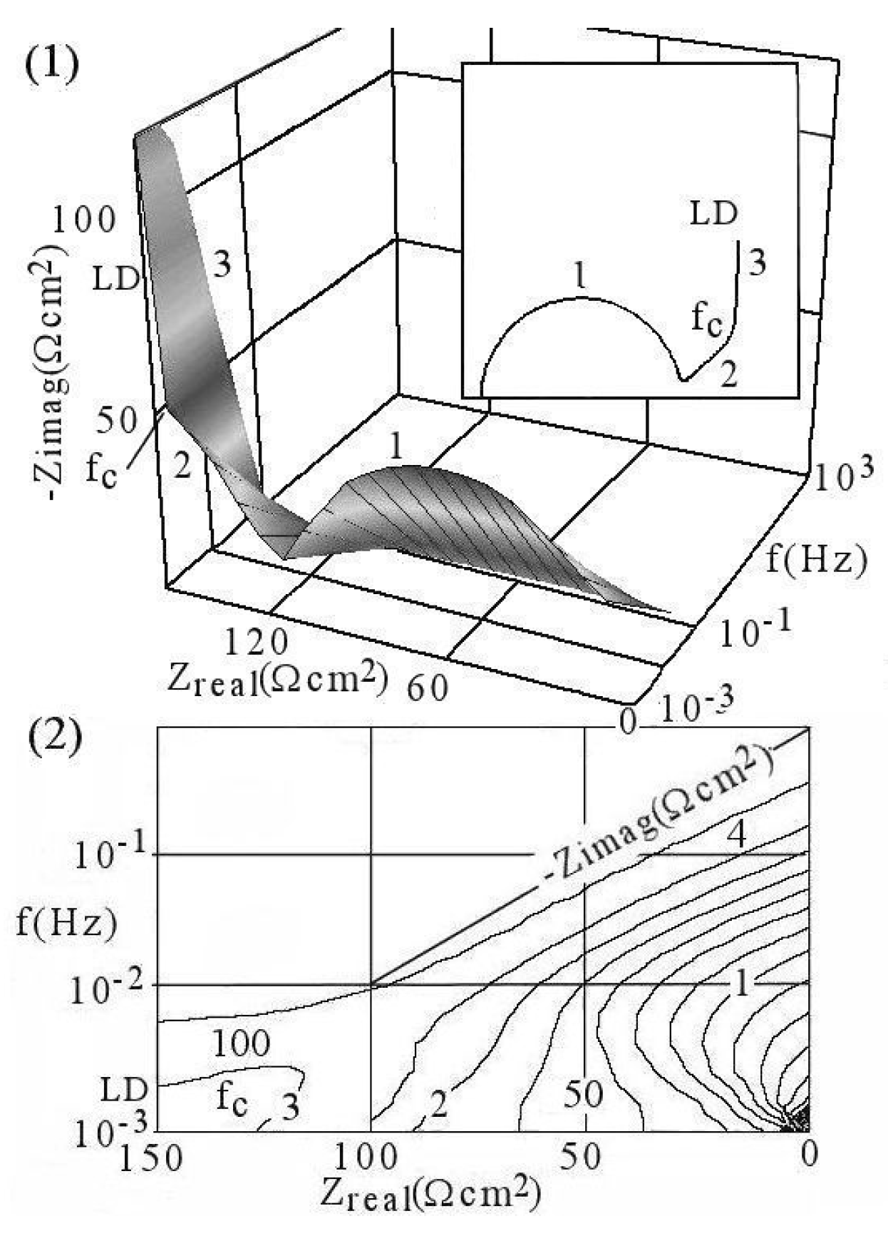
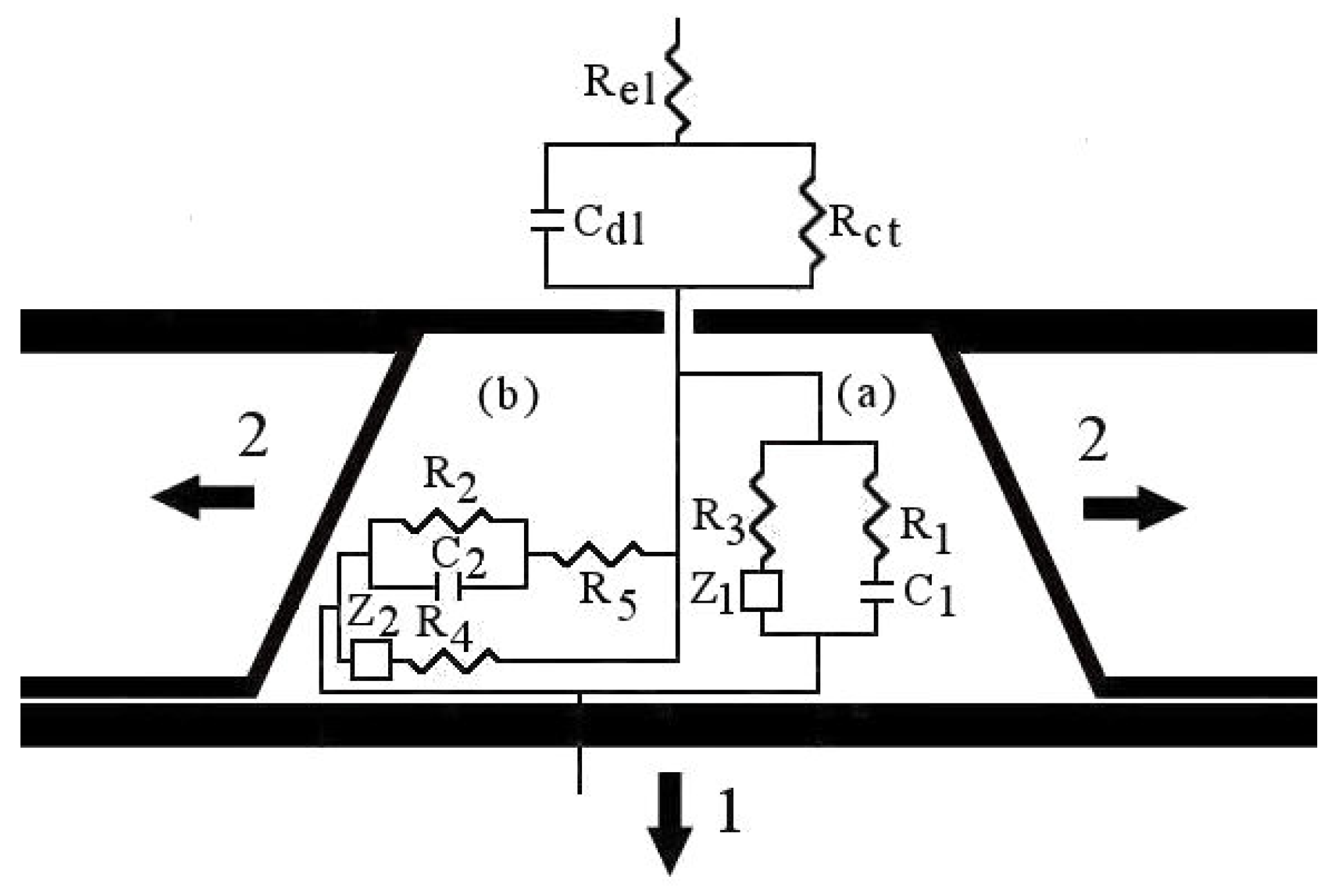
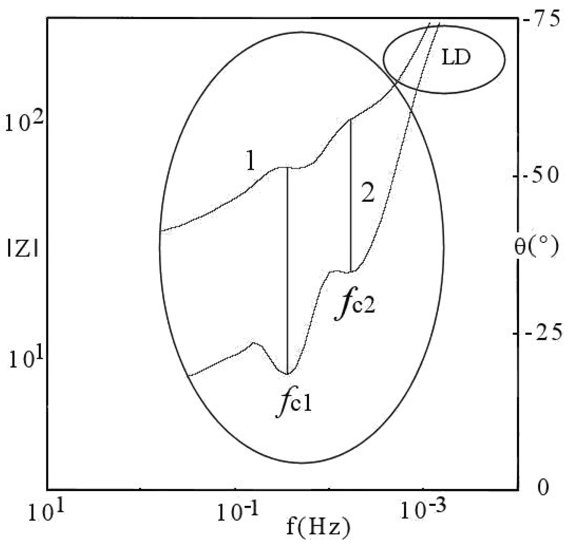
4. Electrochemical Impedance Spectroscopy

According to the voltammetric curve, the experimental impedance diagrams presented in the Nyquist spectra were obtained in 3D and similarly in the 2D dimension in the active region for hydrogen adsorption and diffusion. One of the aims of plotting the diagram was to interpret the presence of the chaotic process as a function of the active region. Based on interpretation [55,56,57], a scheme will be given for the various mechanisms in this region of hydrogen diffusion in palladium. The mechanisms would involve several steps of hydrogen adsorption and by where the layer and hydrogen profusion may also affect on compressive and expansive stress.

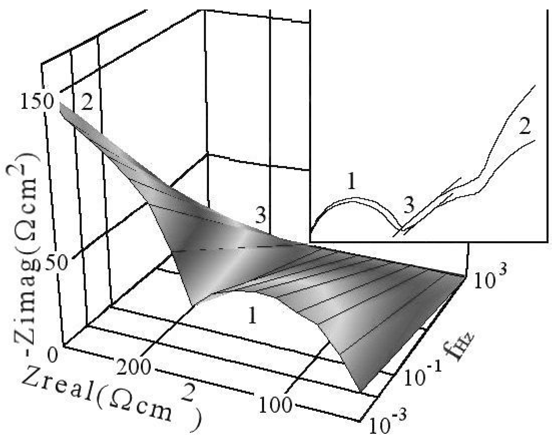
4.1. Measurements in the Reversible Potential

The impedance characteristic obtained for peak A (Figure 2(1) a) can be interpreted as a capacitive adsorption (Figure 3(1,2) event 1) with sub-layer modification (event 4) followed by a diffusion loop (event 2). Examining the blocking diffusion (event 3), there is no detailed model for chaos in the literature. For this reason, this work is focused on describing the concept of chaos. To provide physical significance for the impedance diagram, an equivalent circuit is proposed in Figure 4. The results obtained by simulation coincide with the experimental diagram. In this equivalent circuit, the respective impedances are connected indicating complex adsorption and diffusion. The complex dynamic of diffusion impedance depends on the Warburg diffusion (W) and insertion elements. Blocking diffusion (event 3) comes from microscopic default or sleeping clusters formed during the cold machining of palladium. Releasing mechanical default by annealing should be necessary for correct diffusion. In this perspective, blocking diffusion depth [58] is depicted from the following equation (Equation (1)) [59]:

$$\delta =\sqrt{\frac{3D}{2\pi f_c}}$$

(1)

where $\delta$ is the penetration depth by diffusion and D is the diffusion coefficient taking the usual value 2.4 × 10⁻⁷ cm² s⁻¹ at 20 °C. Diffusion thickness is calculated near the reversible potential, where the Bockris pressure acts for 10⁹ Pa [60]. High pressure can induce compression and stress in palladium, thereby cracking. The characteristic frequency, $f_{\mathrm{c}}$, is at the intersection of the straight line inclined at 45° corresponding to diffusion and the straight line at 90° where blocking diffusion is acting. The simulation results of 65 μm depth achieve the blocking diffusion in this irreversible region. The double-layer adsorption capacitance is 20 μF cm⁻². This low capacitance value appears to correspond to hydrogen transfer into palladium. The characteristic frequency will vary so that surface plays a role in the adsorption of transient and diffusion thickness. At higher frequencies in the spectra, the transfer resistance decreases when adsorption increases. This results from an increase in transfer mechanism inducing easy diffusion before blocking.

4.2. Transient Rearrangement and Overlapping

At the potential between peak A and the beginning of the shoulder B (Figure 2(1)b), the spectra show a capacitive semi-circle and a constant phase element (CPE) separated by a straight line with three different time constants in the Nyquist plot (Figure 5). In these spectra, there is a displacement of the frequency, which can change the appearance of the CPE loop. Transients can be correlated to two capacitances for adsorption (events 1–2) with the Warburg element (event 3) in the equivalent circuit. It is possible that the corresponding CPE would partly hide the Warburg elements to an adsorbed transient. The origin comparable circuit model must represent a good approach to the electrochemical system for reasonable data matching. According to the CPE and low recovery values, the impedance for diffusion in palladium corresponds to nanoscopic adsorption with diffusion in the depth of palladium. It is suggested that the current distribution is not uniform, and adsorption is produced from partial coverage. This circuit first combines adsorption–transfer charge resistance (R₁) and the corresponding capacitance (C₁). Then, the constant phase element (event 2) substituting a depressed semi-circle capacitive varies at low frequency in the imaginary part.

The absorption resistance (R₃) and the Warburg diffusion (Z₁) appear in this circuit, where the CPE can tend rapidly to high imaginary impedance values for low frequencies presaging a blocking diffusion. In Figure 5, the portion of the CPE branch (event 2) can be linked to the processes of transport [61] and should be called a pseudo-diffusion loop. The elongated impedance (event 2) describes the impedance of a finite depth diffusion while forming a short doublet in the position of Figure 2(2)Bb. These diagrams show the system complexity and evolution in the equivalent circuit with hydrogen charging in this intermediate location where the large Bockris pressure is less acting. If the characteristic capacitive frequency is too high, the loop becomes less observable by the fact that this is placed in the high frequency. The same behavior arises for the straight line of diffusion when the frequency is too low. Furthermore, neighboring values for the two characteristic frequencies lead to a coalescence of the CPE loop with the Warburg straight line, which becomes no longer separable and thus unusable. According to the straight line tending to a slope of 45°, the charge–transfer resistance will be high, thereby making the diffusion layer sufficiently thick. It should also be noted that the frequency corresponding to the CPE loop is moving to the low values when its amplitude increases, signifying that depth increases. The capacitive current is thus decreased. The loop confirms the previous hypothesis that adsorbed hydrogen is formed at the surface of palladium for a short time before diffusion and blocking diffusion.

4.3. Measurements in the Equilibrium Potential

In Figure 6, the experimental impedance diagram subjected to hydrogen sorption at the potential on the shoulder (Figure 2(1)c) shows two capacitive semi-circles (events 1–2) and the respective diffusion loops (events 3–4). These semi-circles can be separated by a breaking-point depending on adsorption and double diffusion mechanisms for hydrogen [62,63]. The breaking-point [64] provides time constants related to changing transfer characteristics. It would corroborate the open Warburg impedance and the capacitance of the adsorbed layer. In this case, the electrical schema (Figure 4) is governed by parallel combination leading to the complexity of ramification by double diffusion and competitive absorption (R₃, R₄) with complex arrangement [13]. Two models can be retained for diffusion, one corresponds to diffusion under constraint by hydrogen adsorbate in peak A, and the other corresponds to cathodic diffusion (shoulder B) with hydrogen transients (Z₁, Z₂). These are acting at low frequency. The blocking diffusion corroborates the origin of the vertical line (event 5) after absorption in the reflective interface. In this circuit, the interfacial capacitive impedance is composed of a successive combination ofadsorption capacitances (${\mathrm{C}}_{1,2\dots }$) and resistances (${\mathrm{R}}_{1,2,5\dots }$). Their effect can be seen at medium and high frequencies. According to the resistance and capacitance values, this layer is not considered a barrier for the hydrogen transfer before blocking, where the impedance becomes high at low frequency. Although not directly affected by the diffusion, the capacitive branch would intervene in the process.

In the spectra, the breaking-point is not always visible due to the overlapping of the semi-circle by the straight line, as seen in Figure 6. The Warburg straight lines (events 3–4) signify transmissive diffusion through the palladium preceded by the adsorption reaction at low frequencies. At medium frequencies, the hydrogen adsorbed can be diffused further, or aid the Warburg impedances to appear or disappear. Spectra can be interpreted as competitive phenomena with primary diffusion in the reversible region and secondary diffusion near the equilibrium region (Figure 2(1)a–c) and possible blocking diffusion (event 5).

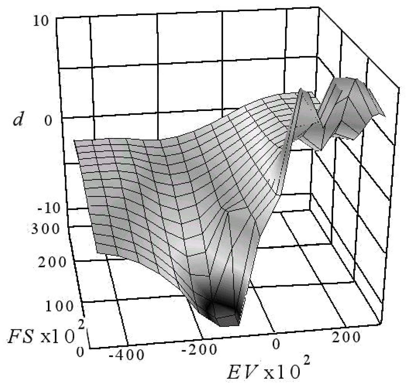
5. Interpreting the Limited Diffusion

The capacitive effect gradually attenuates on these impedance graphs reaching the lowest frequencies. The diffusion results are visible mainly between 10⁻¹ and 10⁻³ Hz. After this analysis, the photograph obtained by SEM microscopy in Figure 7 shows numerous cracks for a few μm in depth near the entry surface (a) and 65 μm in depth near the exit surface (c). These are obtained respectively for the equilibrium potential and the reversible potential. Therefore, it is essential to point out crevices that are strongly dependent on cathode thickness and the time lapses for blocking diffusion. Cracks corroborate the presence of two solid $\alpha$, $\beta$ hydrogen–palladium phases not miscible where the lattice size is changing at low temperature, therefore blocking diffusion in the subsurface and depth. In deduction of SEM examination, the impedance would drop during the formation of the transients, and then this will increase gradually until the blocking diffusion. From the spectra, it was seen that the breaking-point increases when the potentials are shifted to more positive values. The breaking-point increase signifies more absorbed hydrogen accumulated in the subsurface of palladium. This suggests that diffusion would decrease in depth if mechanical defaults formed during machining were not released. It has also observed that the breaking frequency changes with the values of electrical parameters indicating diffusion evolution. The specific frequency shifting to lower values signifies increasing the deeper diffusion. In come-back to Figure 6, the capacitive semi-circles (events 1–2) can be ascribed for two adsorption mechanisms as mentioned in section voltammetry (peak A, shoulder B). Moreover, the breaking-point can be challenging to recognize because it is nearly associated with complex adsorption capacitances and charge transfer resistances. The diagram degenerates in two portions of the Warburg straight line (events 3–4). According to the Warburg straight lines, hydrogen transfer in the palladium cathode occurs via two models of diffusion:

(a)

diffusion by charging mono-atomic hydrogen (Figure 2(1)a),

(b)

followed by diffusion by cathodic complex (Figure 2(1)c).

The comparison shows that the resistance values are higher for the diffusion by cathodic complex. These indicate more difficulty for local diffusion, leading to hydrogen trapping with more considerable stress in the entry surface, as seen in Figure 7.

The diffusion by the cathodic complex appears lower than that obtained by charging mono-atomic hydrogen. These lead to two permeation processes, as seen in Figure 8. Therefore, the diffusion is featured by two dynamics. The two branches can model these in the spectra where the constant times depend on the values of complex Warburg impedance. The permeability (p) can also be related to over-potential ($\eta$), thus the current, whose slopes $\frac{\partial \mathrm{p}}{\partial \eta }$ are, respectively, 0.5 and 0.12. Diffusion by a cathodic complex is progressively produced as a next step, expanding in the subsurface. In the Nyquist plot, the hidden second vertical line corresponding to blocking diffusion in the subsurface cannot be correctly analyzed due to the fact this is too close to the surface. Consequently, the breaking-point depends on the diffusion type, i.e., diffusion by charging mono-atomic hydrogen or beginning of stress by diffusion via the cathodic complex. Diffusion by cathodic complex indicates that the adsorption reaction with a stressed morphology does not guarantee the good mechanical performance of palladium. This demonstration shows that the blocking diffusion becomes limitative at 65 μm depth, and the diffusion impedance behaves like a particular Warburg impedance. Considering the blocking-diffusion in the subsurface, this is effective for a few μm depth. The impedance at low frequencies maintains Warburg behavior, but a capacitive branch is possible at an intermediate frequency. Therefore, the diagram would predict when morphology in the palladium has defaults, when diffusion by charging mono-atomic hydrogen is slow, and when diffusion by cathodic complex is produced (Figure 2(1)a,c). Impedance variation indicates that the diffusion distribution for the palladium is not uniform and not stable. A less deep penetration comes from blocking diffusion and provokes self-induced stress and crack propagation in the subsurface. In this condition, palladium should be rapidly destroyed superficially while a few deep linear cracks cross right through the palladium, as shown in Figure 7 event b and in [12,13]. The electrochemical impedance spectra provide a criterion of stability or instability.

ii-Chaos Analysis

6. DescriptiveInformation of Chaos Analyzer

To access valuable information on the trapped hydrogen and the stresses corresponding to the deformation, simulations were made by a chaos analyzer [65,66]. Chaos and noise have previously been suspected from the electrochemical circuit model [67]. The electrochemical noise impedance measurement is a precursive method to suppose stress cracking corrosion when blocking Warburg impedance is detected. An advantage is the ability to make measurements at low frequencies down to 10⁻³ Hz. The electrical circuit that could give rise to chaotic behavior must include linear elements and at least one nonlinear active Warburg impedance powered by the electrochemical impedance spectroscope [68]. This generator is characterized by frequency whose slope can be negative or positive. Therefore, when using a chaos analyzer, open or close scrolls, loops, and other exciting repulsors and attractor or dynamic phenomena are identified in the Warburg impedance for transients regarding the experimental spectra. Overusing a specific range of parameters, the active system will have periodic or eventually aperiodic orbits. In the case of restricted diffusion, the orbit of chaos, although nominally unstable, would present a helical curve likeness to a trajectory of Lissajous [46]. In this case, a qualitative change should be noted in the system when the dynamic parameters vary. This would involve a difference in the stability with the creation or destruction of one or several orbits or coalescence or annihilation depending on the aspect of diffusion restricted. As the parameters are tuned beyond a critical value, some isolated short bursts would appear more or less frequently among the regular trajectory [69]. The irregular or periodic orbits should make it possible to identify the mechanisms behind this system. In this connection, the Chua circuit presents a richness of classic chaotic behavior to describe the electrochemical reactions [70]. Therefore, to illustrate the trajectory, the reaction sequence of the adsorbate has to be taken into account for diffusion [71]. Considering the front profile for two hydrogen adsorbates on the recovery space, $r$, Equations (2) and (3) are:

$$\frac{\partial x}{\partial E}=\alpha \left[y-g(x)\right]+D_x\frac{{\partial }^{2}x}{{\partial }^{2}r}$$

(2)

$$\frac{\partial y}{\partial E}=\beta \left[x-y+z\right]+D_y\frac{{\partial }^{2}y}{{\partial }^{2}r}$$

(3)

$$\frac{\partial z}{\partial E}=-\gamma y$$

(4)

where x, y and z intermediate species represent the front profile of adsorbates on palladium, including three models for hydrogen adsorbed and diffused and one for the adsorbed oxide (z). E is the potential depending on kinetic, $\alpha$, $\beta$, $\gamma$ and x,y are parameters. It is possible to have combined models for x (model 1) with y (model 3) represented by x,y (model 2). The solution of equations makes it possible to obtain positive and negative values of the variable [72]. D_x and D_y are the shared hydrogen diffusion coefficient for adsorbate x and y. A linear transformation converts the electrical system into a template for a dynamic electrochemical field.

Equation (5) obtained from [73] represents the limiting diffusion impedance, j is the imaginary part, and f is the frequency. The limiting diffusion impedance (LDI) can be expressed by taking into account the two adsorbates and the limiting diffusion (LD):

$$Z_{{\mathrm{LDI}}_{(x,y)}}=-\frac{1+\frac{2j\pi f{\delta }_{(x,y)}^2}{3D_{(x,y)}}}{2j\pi f{\delta }_{(x,y)}F\frac{\partial C_{{(x,y)}_{\mathrm{ads}}}}{\partial R_{\mathrm{ins}}}}$$

(5)

where $C_{{(x,y)}_{\mathrm{ads}}}$ is the adsorbate content defined by cyclic voltammetry. The characteristic diffusion impedance is obtained from the electrochemical impedance spectrum (Bode plot, Figure 9). In Equation (5), it can be seen that there is a response of diffusion thickness for adsorbates governed by the steady-state or unstable state. If the variation of diffusion impedance is converging, the system tends to be stable [67] (pp. 133–136). Conversely, the system is unstable. According to the Bode spectra and Equation (1), for the characteristic frequency, $f_{c1}={2\times 10}^{-2}$ Hz the blocking in the subsurface is ${\delta }_1$ = 16 μm, and for the second characteristic frequency $f_{c2}={5\times 10}^{-3}$ Hz the blocking in depth is ${\delta }_2$ = 65 μm. Cathode membrane of thickness less than 65 μm should be free of restricted diffusion in-depth. Thus, it will be beneficial for permeation at the reversible potential. Therefore, chaos is examined at low frequency where blocking diffusion is produced after adsorption. Considering Equations (2) to (5), different chaos models are possible according to essentially six parameters. These are two for adsorbed species, two for diffusion, one for oxidized palladium, and one concerning the position in the active potential considering scanning voltammetry. Under the appropriate electrochemical reactions and blocking diffusion conditions, chaos can present orbits corresponding to a heterogeneous distribution of adsorbates in an unstable state over a potential region. Their distribution would thereby produce various oscillations. When varying a parameter, a series of the quasiperiodic route of chaotic oscillations are expected. The trajectory of the derivative is not stationary for blocking Warburg impedance. At this stage, the system becomes periodically unstable. The resulting graph would demonstrate the feasibility of analysis for the adsorption–diffusion system with chaos.

To comprehend the chaotic events produced by the dynamical adsorbates, the path of the raw data was examined. The investigation concerns the variation of the derivative between the limited diffusion impedance and the frequency ($\partial Z_{(LDI)}/\partial f$) during instabilities. Several signals would be found involving a single or several transitory moving in two or three dimensions. This number of chaotic and non-chaotic events will be to corroborate the equivalent circuit. In this way, the standard methods of chaotic series analysis as the power spectra, the Fourier series, and the dominant frequencies with the correlation and divergence coefficients are suited to the problem of distinguishing between chaotic and non-chaotic dynamics [74]. In this case, it is shown that orbits play an essential role in these electrochemical models. Effectively, their different characteristics for chaotic and non-chaotic models can interpret events in the palladium–hydrogen system. Results have to be relevant to simulation to verify the existence of chaotic and dynamical properties in the diffusive system. In other words, the corresponding system can be chaotic and obey diffusion equations in x and y. Although the function of Warburg impedance may assume many shapes, the original Chua circuit specifies chaos when instabilities are produced. Chaos is a robust dynamical physical phenomenon sensitive to dependence on evolutive conditions.

This dynamical system will have to depict the differential equations (Equations (2)–(4)). Equations can specify the behavior of impedance over a given short period (or sector) of frequency. To determine the system behavior for a more extended period incorporating the blocking diffusion, it is necessary to integrate all the routes after having applied iteration via the mathematical derivatives using the program such as Chaos Data Analyzer. The dissipative system tends to arise in blocking diffusion in the model, thereby the permeation would cease. The dynamical system corresponding to the electrochemical hydrogen diffusion can be interpreted as an attractor. Examining the derivatives, the repulsor can move away from its origin (divergence), and it can be followed by an attractive affinity converging in the initial point of the phase-space. According to the two adsorbed hydrogen, this system depends on the Warburg impedance (Figure 2(1)a–c). Dissipation in the derivatives can come from blocking diffusion in palladium by dissimilar transients. In contrast, progressive attenuation or harmful derivatives can come from the return of stability. In this case, the driving electrochemical energy to produce the diffusion balances the transients and sets the system into a typical behavior.

In this sense, voltammetry and impedance in the Nyquist or Bode spectra give rise to the complicated interpretation of chaos displaying several routes for the appreciating of dynamic and blocking diffusion. Our objective is to report chaotic phenomena from the actual impedance circuit proposed for hydrogen adsorption and diffusion in palladium. Furthermore, the purpose of analyzing the chaos data is to determine the threshold where instability begins and when the system becomes periodically stable. In this aspect, the adequate instability data analyzer and Fourier analyzer are designed to have access to hazardous activities from the raw data or derivatives data in the limiting diffusion impedance. It makes it possible to obtain matching between phenomena in the Chua circuit. In the fluctuating data, repulsors or attractors form different structures for hydrogen diffusing in stable or unstable palladium hydride. This analysis offers an invaluable assessment of the deterministic characteristics of the system, and can be used to discriminate stability and stress. In the following, the construction of chaos is obtained by using these three transients.

7. Analysis of Models and Result Projection

7.1. Measurements in the Reversible Potential

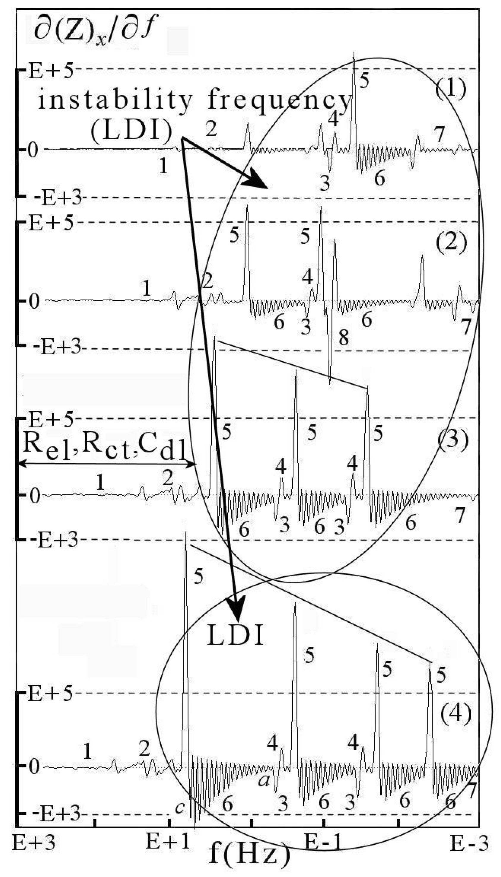
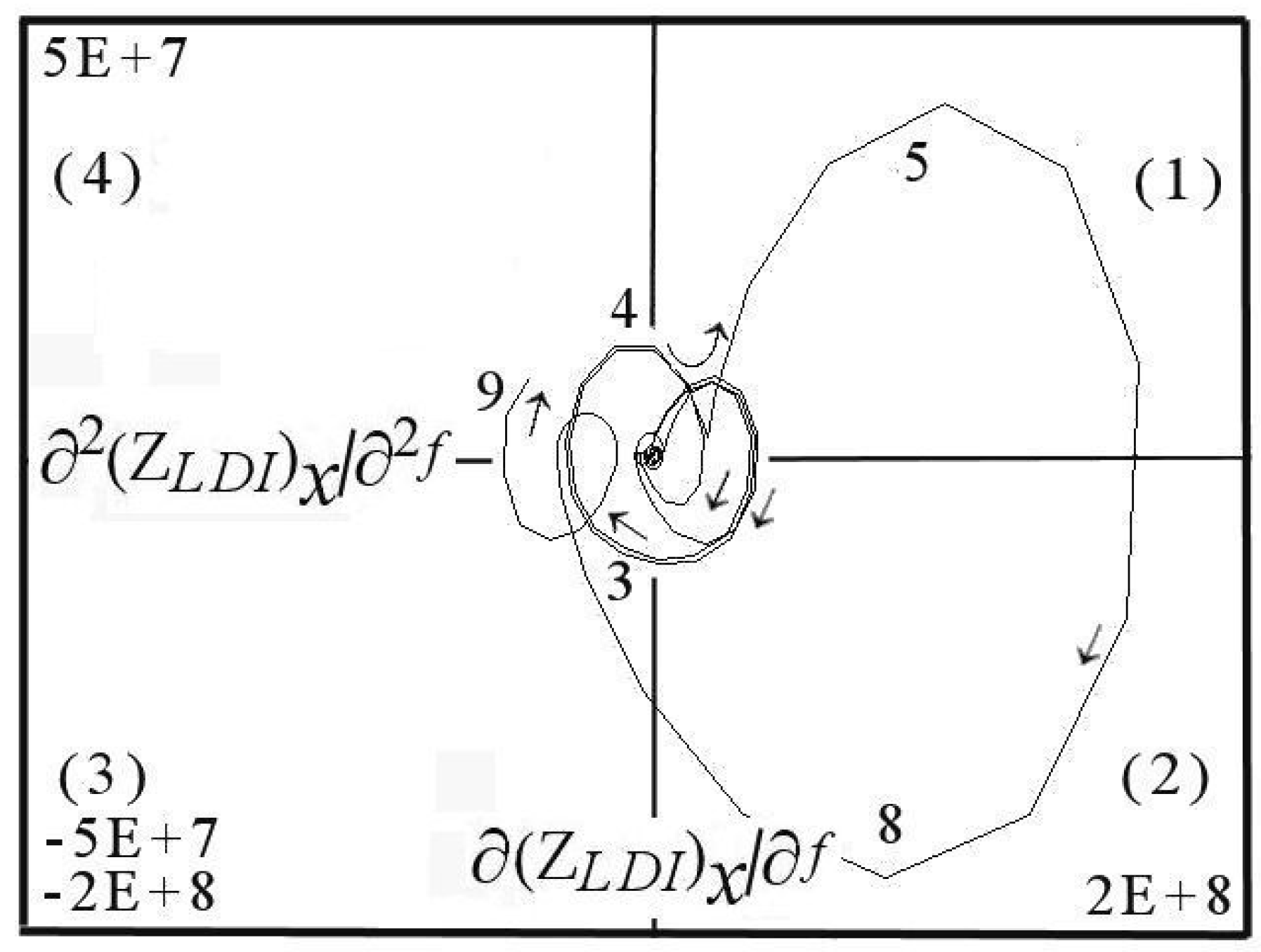
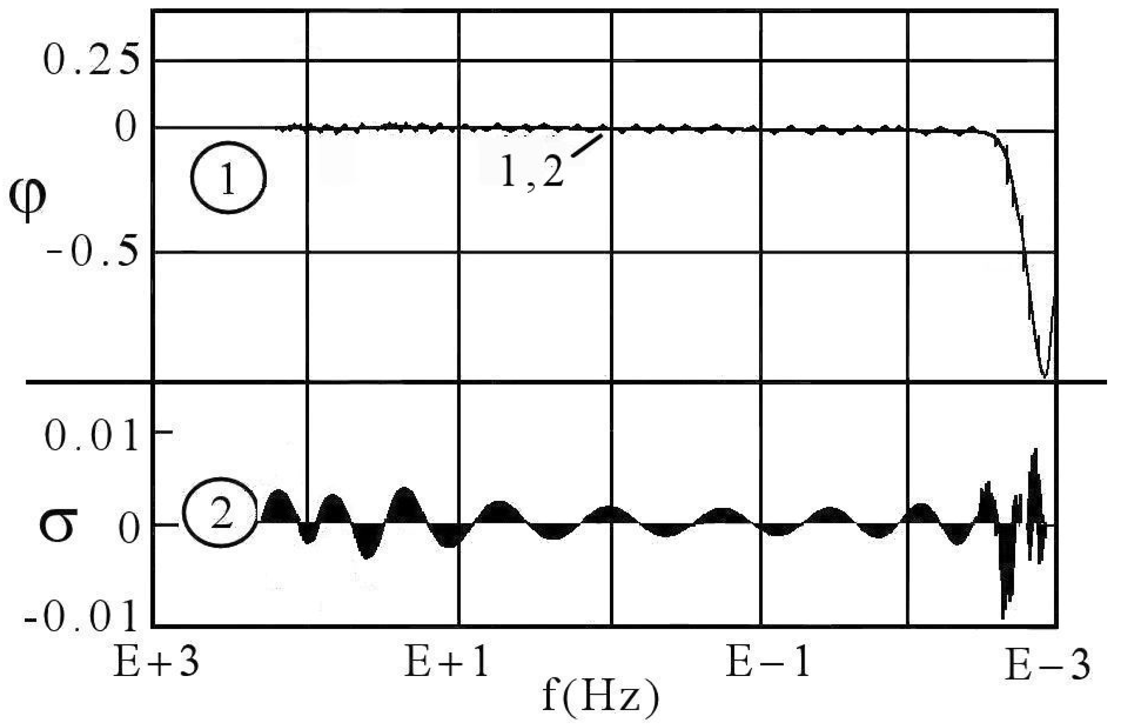
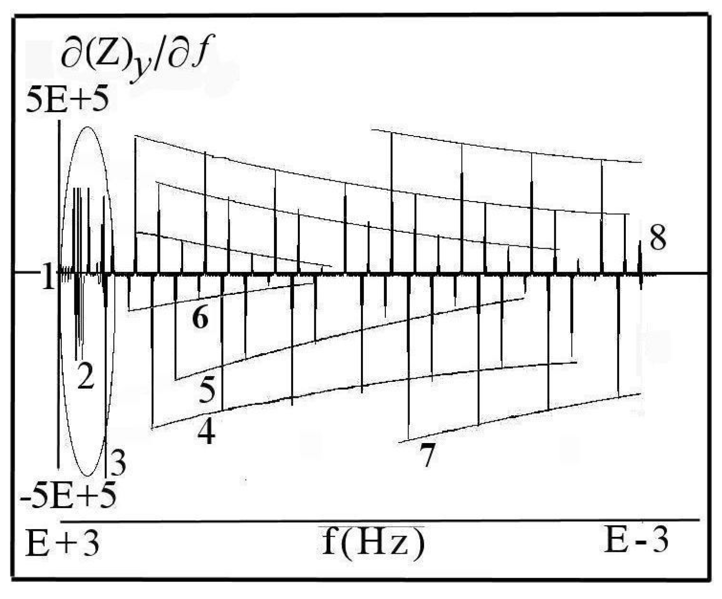
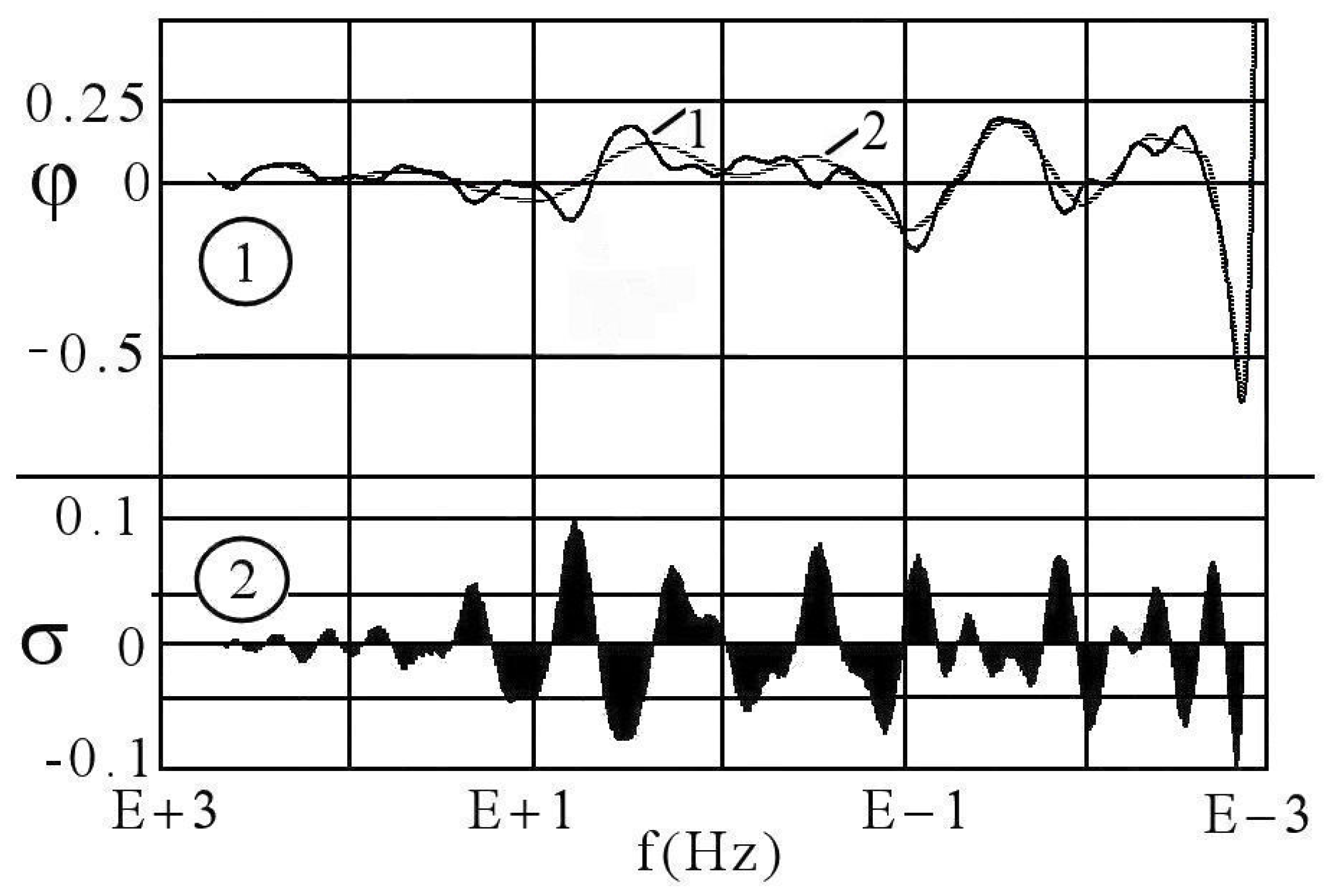
7.1.1. Aspects of Global Spectra

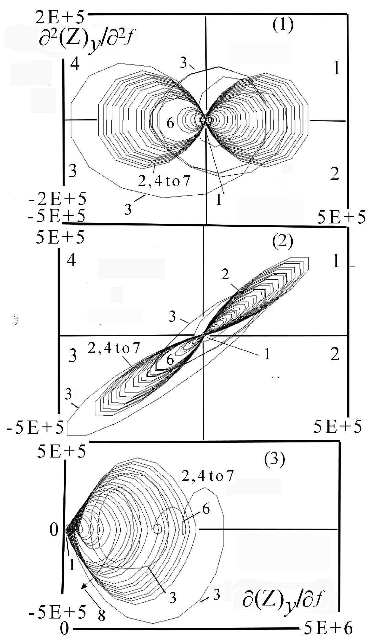
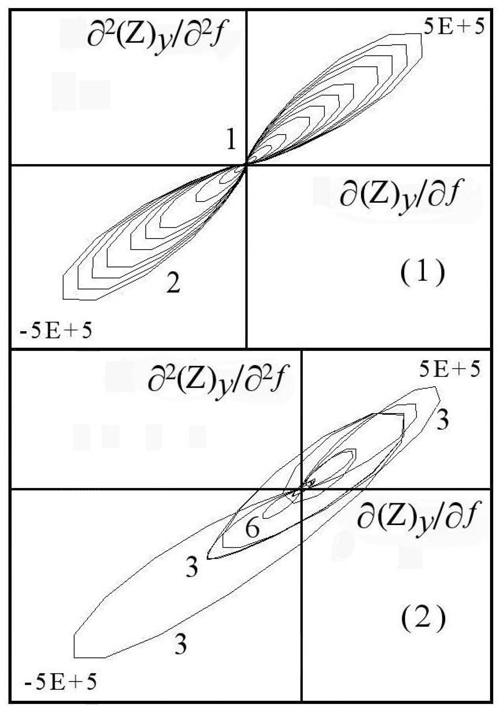
Using Chaos Data Analyzer, Figure 10 shows the unstable events for charging hydrogen (x) after adsorption at low frequency. In this experimental figure, the x-axis represents the frequency whose limits are determined by the analyzer to obtain valuable chaos results. The y-axis is the relationship between the first derivative of impedance ($\partial {\mathrm{Z}}_x$) and the iterated frequency ($\partial f$). At low frequency, limiting diffusion impedance depends on limited depth for diffusion (Equation (1)). The derivative makes it possible to differentiate rising and falling short-lived events between two adjacent impedance values.

This equation corresponds to a response of the variation of adsorbate governing the steady-state or unstable state on the limiting diffusion impedance. Graphs in this figure can depict five types of positive and negative signals. These are:

(a)

continuous line corresponding to capacitive and resistive effect (event 1),

(b)

minor positive instability and negative signal (events 2 to 4),

(c)

significant instability scaled highly positive (event 5),

(d)

which could be synchronized with negative signal (event 8),

(e)

decreasing small negative periodic oscillations (event 6),

(f)

and possible metastable line before stability (event 7).

These graphs describe comparative high and tight pulses in the derivative data. High positive pulses in the y-scaling correspond to the diverging blocking diffusion state with high complex local impedance. At the same time, the negative pulses signify converging complex impedance where diffusion is possible. The nil value in the core corresponds to the stationary state for diffusion. During fast diffusion before blocking, electrons moving in palladium will be intense, thus causing electrical charge transport. In another way, when diffusion is blocking, the diffused electrons can accumulate into the diffusion barrier (event 5) with unstable and high energy. If the blocking barrier disappears in the next step, these are released by event 6, followed by a steady-state for diffusion (event 7). Therefore, the regime can be semi-permanent, periodic, or non-periodic depending on the position of limiting diffusion on the graph of Figure 10. It is possible to decompose these signals into Fourier series and use the Hilbert vector to separate each frequency event.

In Figure 10, the spectra are dominated by the transient impedance occurring when stress cracking nucleates, propagates, finally dies, as explained for an industrial module. Regarding to the positive perturbation up to E + 8 (event 5) followed by cyclic negative oscillation up to −E + 3 (event 6), the transient is formed in this area and will impact the kinetic of chaos. Either the chaos will stop, or it will continue to progress. The signals may also indicate continual cyclic destabilization followed by a repair process coupled with propagating stress. This stress cracking corresponds to a steadily increasing instability during the growth phase (events 4–5), which then falls as the cracks close themselves when $\partial Z_{{(LDI)}_x}/\partial f$ is nil (Figure 10 events 6 to 8). It is undeniable that the repair process gives rise to regular decreasing negative oscillations. These events are hardly detectable by voltammetry or electrochemical impedance spectroscopy. Their measures are not sensitive enough. The self-repair process of the cathode was observed by visual observation at the dismantling of the industrial electrolyzer.

Increasing the absolute negative potential in voltammetry, and consequently growing hydrogen amount in palladium, the intermittent chaotic instability and oscillation change with four periodic sequences (Figure 10 graph 4). These disappear and reappear one after the other as seen in events 5–6. Regarding the more instabilities shared with oscillations, transients should be formed globally on the base of multi-adsorbates (Figure 2(2)Aa). Consequently, the initiation of electrochemical stress is due to sufficient amounts of adsorbed hydrogen observable by impedance instability. Revisiting Figure 10, at high frequency, there is no high variation of raw data demonstrating equilibrium during capacitive adsorption or double-layer preceded by the electrolyte resistance (event 1). Then, tight and high sharped positive pulses are produced, followed by numerous small periodic negative oscillations shaped as a resonant frequency [49]. These intermittent oscillations are reproducible in sequence and illustrate continual nucleation of the repair process for unstable species accompanied by electrochemical stress in the region near the reversible potential. In this region corresponding to the transfer impedance, hydrogen charging is more consequent than at more positive potential. Examining Figure 10(2–4), the synchronized fluctuations give a discernible structure in a well-defined wave-form period where a spiral indicates a periodic system combined with a sharped system. The significant instability and amplitude variation are not trivial and depend on the potential and frequency position. Regarding to potential imposed, the number of unstable events at low and medium frequencies increases when the amount of hydrogen released increases. Moreover, the negative periodic oscillations increase of E + 2.5 as the major instability starts at a higher frequency (events 5–6) when hydrogen amounts are more important (Figure 10(1–4)). Integrating the positive and negative values shows that these are equal, signifying that events 5–6 cannot be dissociated.

It is well known that the Chua circuit can generate a large variety of chaos structurally simple but dynamically complex, consisting of one or more events in the phase-space portrait. Hence, this circuit is frequently encountered in the analysis of derivative to design chaos. The Chua circuit can be incorporated in the complex Warburg impedance in this specific case. The other classical elements, such as capacitor and resistor, have a weak influence in the chaos at high frequency (zero value). In this circuit, chaos implies that data vary. In particular, a dynamical chaos system is characterized by a dense collection of periodic or aperiodic loops or scrolls sensitive to the initial value in the raw data (Figure 10(1–4) events 5–6) so that instabilities can evolve quickly into different states. However, despite a regular appearance, chaos is in a deterministic evolution. In addition, no periodic loop may survive in the boundary data (event 7) after sufficiently strong perturbation in a chaotic system. This is mainly for events 5 or 6 where the periodic oscillations $\partial Z_{{(LDI)}_x}/\partial f$ decrease to fall in the core signifying repair process.

The phase-space in the lateral global view of Figure 11 is a picture of how the Lyapunov exponent evolves. If the values move away from each other, the system becomes unstable. To know how the frequency acts, it is necessary to analyze sections of it. From Figure 11(1–3) corresponding to Figure 10(1–4), typical evolution of the phase-space derivatives (${\partial }^{1,2}Z/{\partial }^{1,2}f$) for the raw data of instability shows that the trajectory forms in first a positive loop (event 5). Then, the trajectory (event 6) turns on itself along an axis to become like a funnel. The trajectory starts from the high value of $\partial Z_{{(LDI)}_x}/\partial f$. When the rolling-up becomes minimal in amplitude (event 7, $a$), the trajectory leaves the funnel and forms a new positive loop (Figure 11(2,3) event 5). A negative loop (event 8) at the bottom can be observed on leaving this event as the trajectory has changed. The disturbance in a positive and negative values of ${\partial }^2{Z}_{{(LDI)}_x}/{\partial }^{2}f$ represents unstable adsorbates followed by the repair process (events 5–8). Then, the trajectory renters in the events 3–4. Some chaotic repulsor–attractors can work with a loop and toroid when viewing the trajectory by the derivative ${\partial }^3{Z}_{{(LDI)}_x}/{\partial }^{3}f$ in equatorial projection (Figure 11(2)). Effects can be diagnosed by analyzing the angle between the phase-space and the third axis. It was experimentally established for the positive angle, and the oscillator corresponds to a typical unstable structure. Consequently, adsorbates will be examined by the power spectrum.

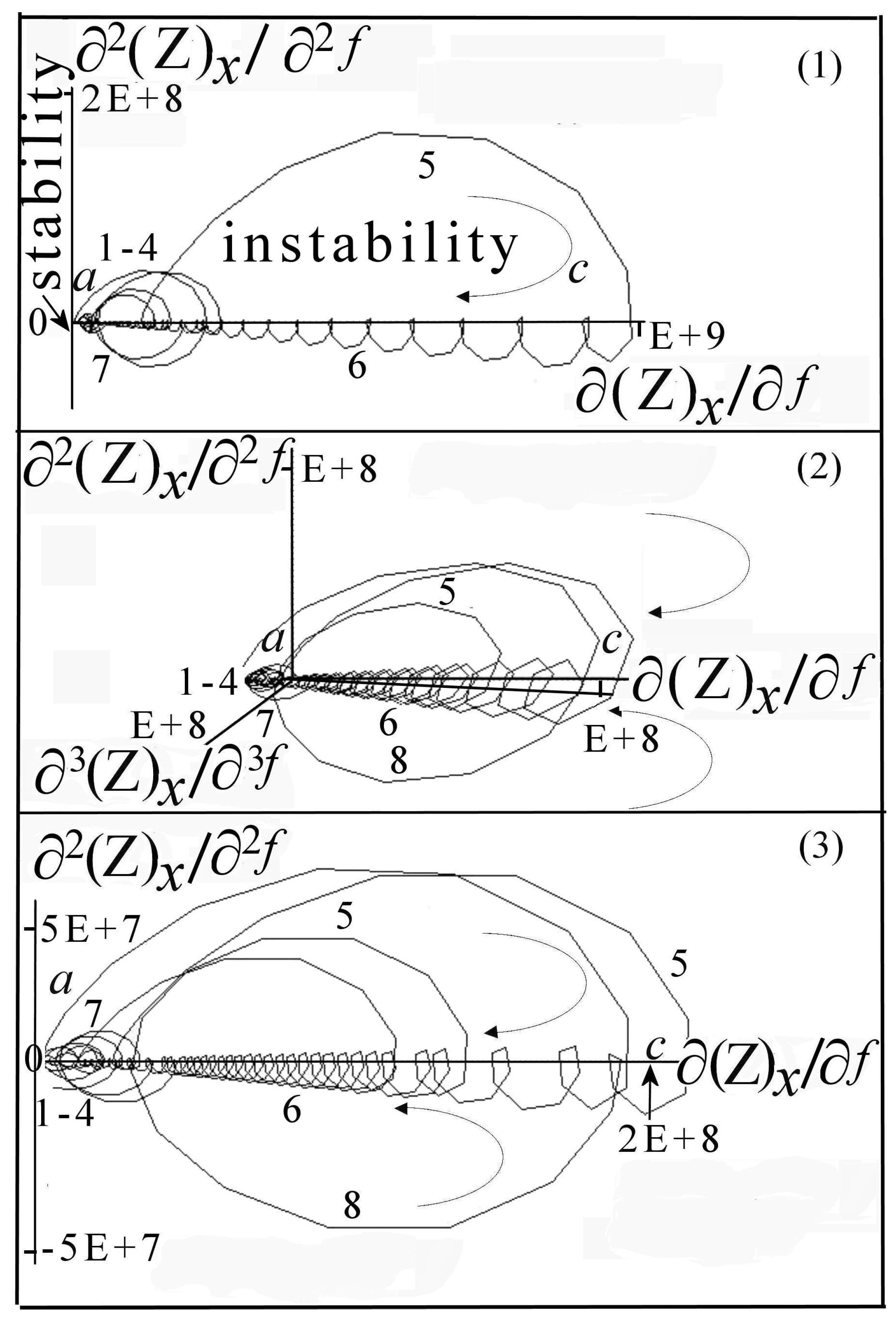
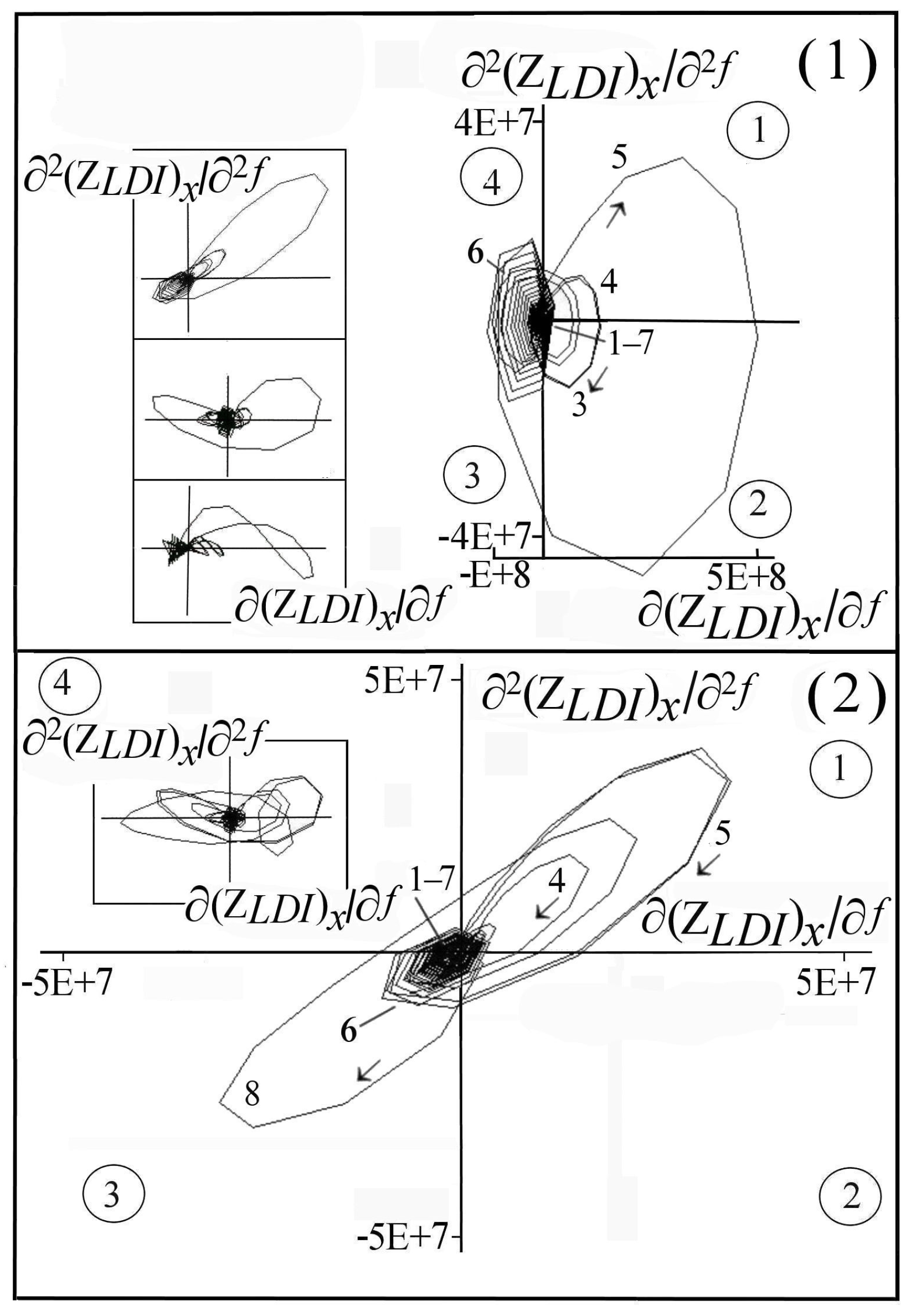
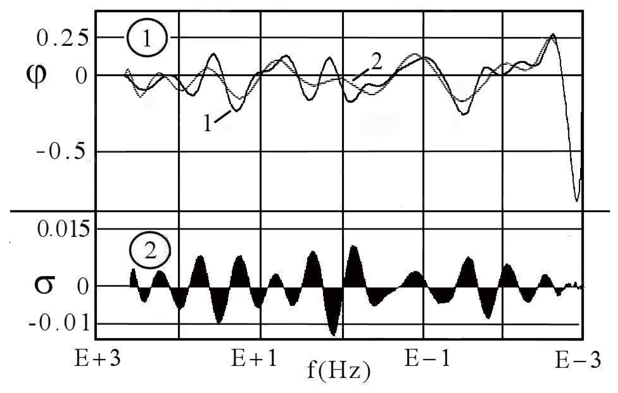
7.1.2. Aspects of Local Sectors in Spectra

After looking at the global spectra, iteration at the low frequency between 10⁻¹ and 10⁻³ Hz has been made in two particular sectors to distinguish the different noises. Model 1 was chosen to represent the reversible potential where hydrogen atoms are charging the palladium with constraints (mechanism Volver):

$$\mathrm{k}{\mathrm{H}}_2\mathrm{O}+\mathrm{Pd}+\mathrm{k}{\mathrm{e}}^{-}\to {\left[{\mathrm{PdH}}_{\mathrm{k}}\right]}_{{\mathrm{ads}}_{(x)}}+\mathrm{k}{\mathrm{OH}}^{-}$$

(6)

Chaos can be predicted using the dynamic characteristics generated by the electrochemical events. In this Equation (6), k is a variable depending on the adsorbate. According to Figure 11, simulation on the modified Chua circuit with attractor–repulsor is presented for event 6 in an angular view of Figure 12A. In this figure, the data derivative is, in turn, positive or negative then tends to zero. The Lyapunov exponent allows for estimating stability in exploring the phase-space derivative (Equation (7)). The stable-state is determined by the difference of ${\left[{\partial }^2{Z}_{(LDI)}/{\partial }^{2}f\right]}_{2-1}$ between two neighboring ${\left[\partial Z_{(LDI)}/\partial f\right]}_{2-1}$:

$$\lambda =log\frac{{\left[{\partial }^2{Z}_{(LDI)}/{\partial }^{2}f\right]}_{2-1}}{{\left[\partial Z_{(LDI)}/\partial f\right]}_{2-1}}$$

(7)

$\lambda$ can be negative or positive according to the logarithmic values of the impedance vector. A graphical example to calculate is given in the frontal view of Figure 12(B-windows) events 1–2 using the $\partial Z_{{(LDI)}_x}/\partial f$ raw data (x-axis) and ${\partial }^2{Z}_{{(LDI)}_x}/{\partial }^{2}f$ derivative of the phase space (y-axis). This equation commonly refers to a global exponent determining the predictability throughout the dynamic system. Along with the global indicator of chaos, there are the local indicators that are more precise and clearly show whether a signal is locally chaotic or not. They offer an analytical criterion for stability. In Figure 12A, the ${\partial }^2{Z}_{{(LDI)}_x}/{\partial }^{2}f$ derivative satisfies the variation of the local Lyapunov exponent. The local exponent allows for predicting the stability around a local segment in phase-space. If one of the Lyapunov exponents is positive and if the system is regular, then the equilibrium point is unstable. For this figure, the local Lyapunov exponent is variable and is depending on its position on a spiral: +1.668, +1.030, +0.800, +0.306, −0.001, −0.246 and −0.620 (Figure 12(C-windows)). According to the results, the eigenvalues are stable at high frequency, whereas variability is seen at low frequency. These coefficients can be organized on a curve to study how the divergence and convergence are at a metastable point of equilibrium depending on the dynamic. This system is called bounded because an exponent is negative and close to the equilibrium point (−0.001 at $a$).These significant numbers denote complexity of the encountered chaos in this system. The mathematical point of concentration at the origin of the axes in the phase-space will be called “eye” in the core. In the negative core of chaotic behavior, the Lyapunov exponent suddenly increases positively to +1.668. This corresponds to point $c$ in the funnel (Figure 11 and Figure 12). It is clear that values change, and the exponent is like an estimator of chaos. The large amplitude variations agree to highlight a periodicity domain corresponding to chaos and repair areas. This signifies a degree of disorder followed by a degree of order and vice versa. Extrapolation of the results for the Chua model suggests that the functions in Equations (2) and (3) are correlated with Equation (5), and may reflect variation in the Lyapunov exponent (Equation (7)).

Synchronization occurs when all conditional exponents are negative, but the Lyapunov exponent cannot be carried out analytically in all cases. In this case, during hydrogen adsorption and diffusion, the derivative phase-space consists of positive or negative multiple orbits with smaller and smaller cyclic positive or negative oscillations representing impedance variation (Figure 12A, first and third quarters). The rapid convergence of oscillations towards the “eye” indicates the diffusion of hydrogen. Therefore, during diffusion, the attractor–repulsor can present a positive or negative toroid of more or less low periodicity. Consequently, the Lyapunov exponent is not a negligible parameter characterizing the properties of attraction or repulsion for the dynamical diffusion. It measures the convergence or divergence rate in measuring infinitesimal intervals of nearby two close trajectories (Figure 12B). The trajectory can take different orientations in phase-space. Depending on the data, attraction or repulsion, it is possible to predict the chaos. The higher positive Lyapunov exponent quantifies the greatest rate of instability when the distance between two nearby positive trajectories increases. When the Lyapunov exponent is zero, a stable steady-state should exist, whereas, if the exponent is negative, the system is converging with more possibility of stability formation in diffusion. Iterating the mapping of the phase-space, if its value is slightly positive, the predictability of the trajectory along orbit cannot be guaranteed. The attractor can exhibit more or less stable behavior. In case of difficulty for interpretation, examining a come-back towards a steady-state by convergence into the core should be useful and inversely.

In Figure 12A, event 6, Lyapunov exponent value is in first highly positive by divergence. There is a fast come-back towards origin followed by divergence showing that the system is first of all unstable. When event 6 converges, the decreasing spiral system should temporarily become stable. It quickly tends towards a negative value or zero in returning to the x–y axes origin where diffusion is stable. Its electrochemical behavior corresponds to stability in the “eye” where nothing happens. In this case, the local Lyapunov exponent is −1.490 for event 6, indicating the convergence in this “eye”. In events 4–5 in Figure 13, the local Lyapunov is 1.030 and the Eigenvalues are 1.273, −0.243, and 2.043, indicating divergence.

To distinguish chaotic repulsor for events 4–5 in Figure 10 and Figure 11, another local sector is presented in Figure 13. Trajectory diverges essentially in the first quarter. It forms tight and unidirectional double loops (events 3–4) and finally presents a Chua circuit open-loop for an unstable orbit (event 9). Local Lyapunov is 1.668, and this corresponds to a metastable event. As soon as diffusion is a few blocking, irregular directions appear along with the orientation of coordinates of ${\partial }^2{Z}_{{(LDI)}_x}/{\partial }^{2}f$. According to the phase-space plot in-plane projection obtained by changing the perspective drawing (Figure 14), the trajectory spirals up to the core in the central axes.

The oscillation frequency increases, forming a double-orbit in the positive first and negative second quarter (Figure 14(2) events 3 to 5). More explicitly, if the trajectory enters in the negative third quarter ($\partial Z_{{(LDI)}_x}/\partial f$ and ${\partial }^2{Z}_{{(LDI)}_x}/{\partial }^{2}f$ coordinates are <0), the local Lyapunov is negative and corresponds to stable, tight converging spirals (events 6 and 8)—or, if it enters in the first quarter ($\partial Z_{{(LDI)}_x}/\partial f$ and ${\partial }^2{Z}_{{(LDI)}_x}/{\partial }^{2}f$ coordinates are >0) where the local Lyapunov is positive, this corresponds to the unstable scrolls (event 5). In Figure 14(1,2), the $\partial Z_{{(LDI)}_x}/\partial f$ and ${\partial }^2{Z}_{{(LDI)}_x}/{\partial }^{2}f$ coordinates provide a strong signature for stability or instability. From these figures, when trajectory comes back again in origin, complete zero crossing is seen. This presents a system of close-loop Chua circuit eventually with double-orbit, where the stable orbit is in the “eye” forming a dense collection of periodic orbits (where event 6 becomes nil). To improve the readability in Figure 14(2), phase-space was drawn episode by episode (Figure 15). This figure shows a continual variability of divergence and convergence during the consecutive episodes.

Such consecutive episodes are associated with the black tight and centered orbits (events 1 and 7) inside the core in the $\partial Z_{{(LDI)}_x}/\partial f$ - ${\partial }^2{Z}_{{(LDI)}_x}/{\partial }^{2}f$ projection (Figure 14 framed windows). Windowing refers to selecting a frequency sector to reduce the spectrum’s spreading. In the windows realized in spatial projection map mode, the trajectory presents a misshapen spiral emerging from event 6. Such behavior follows divergence in event 5 and convergence (events 6–8). As soon as the diffusing hydrogen is a little disturbed, disorderly directions appear along the equatorial axis of $\partial Z_{{(LDI)}_x}/\partial f$. Framed windows show the distorted chaotic events from regular periodic orbits to the “eye” of the trajectory (events 1 and 7) where the local Lyapunov returns a negative amount (−1.490) and indicates the stability of the variable. In this case, precarious equilibrium synchronization between existing transients ${\left[{\mathrm{PdH}}_{\mathrm{k}}\right]}_{ad{s}_x}$ should be due to stable interconnection between them where the Lyapunov is negative towards the “eye” (−1.356). The eigenvalues are 0.97, −1.43, and −1.47. There is a negative Lyapunov and two negative eigenvalues. These suggest that the system is metastable and driven by harmoniously coordinated dynamic, except where the Lyapunov exponent is positively high and where there are three positive eigenvalues. These converging orbits can be regarded as a pattern. This reinforces the idea that topological analysis of the phase-space derivative is fruitful in revealing the level of organization of unstable and stable systems. Distorted scrolls become visible in Figure 14 framed windows depending on the viewing angle. Distortions are related to the dynamic of anomalous and blocking diffusion of hydrogen in palladium. These reflect the complexity of the system. According to these results, the proposed impedance circuit is semi-periodic but highly chaotic. Stability is only obtained in the “eye” after passing the funnel.

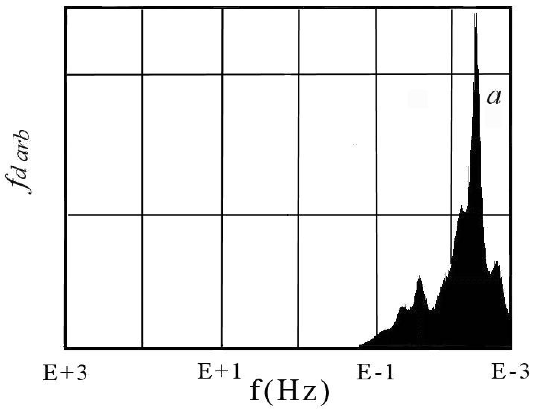
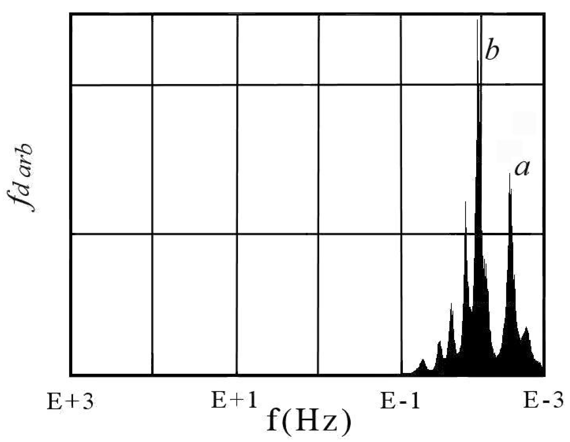
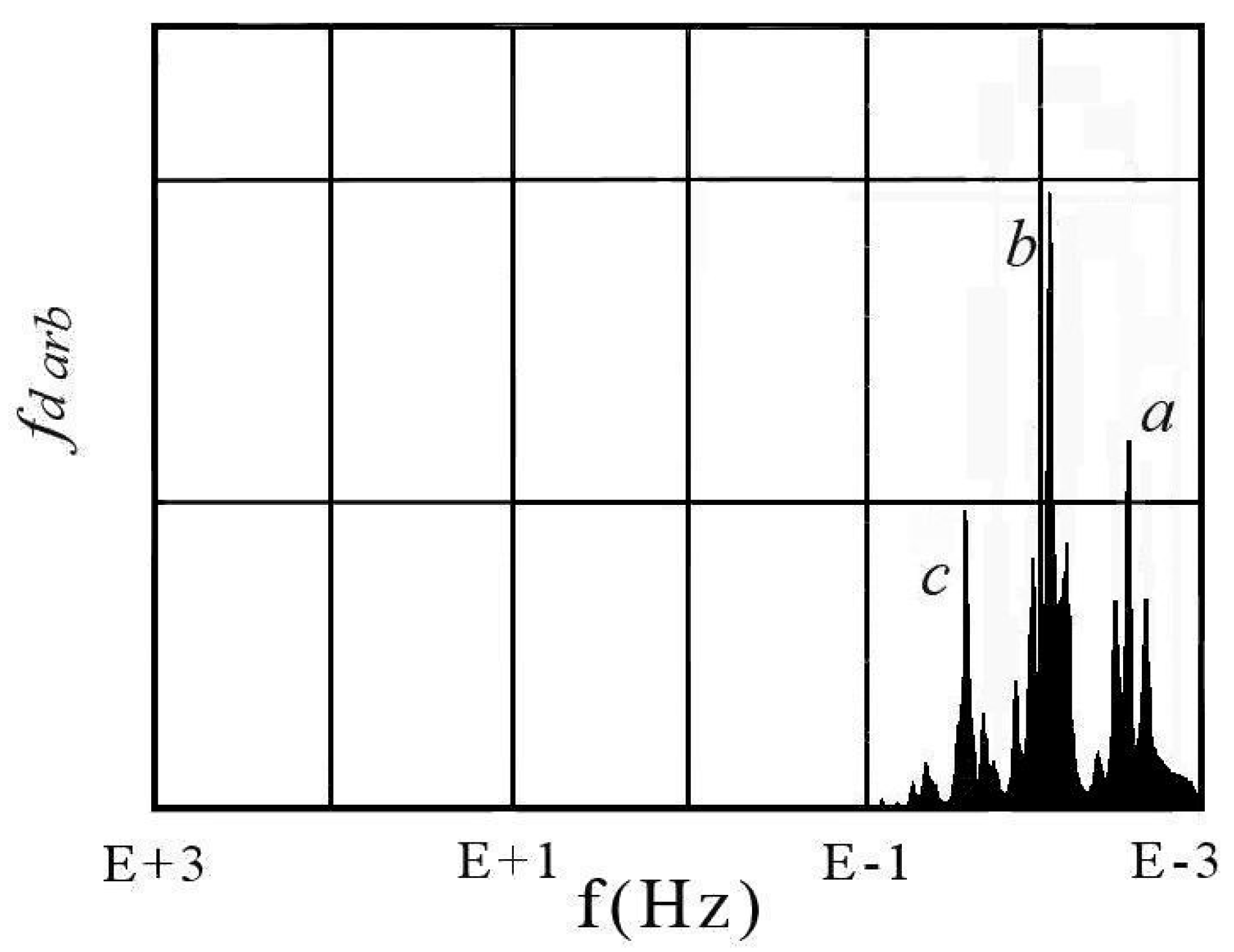
7.1.3. Aspects of Power Spectra

The power spectra can estimate changes in the Lyapunov exponent, thus assessing the level of chaos. The properties of chaotic events in the phase-space derivative depend on the frequency. For that, spectral analysis has to play a crucial role in locating and representing the significant peak of energy corresponding to the transients to understand the property of a non-stationary signal [75,76]. However, it cannot be easy to interpret them, and they must be appropriately evaluated. The main problem is that, when using a polynomial function to discern the different events, the evolution of signals has to be followed. Therefore, analysis has to locate these events occurring in the impedance spectra. The power spectra should show the presence of significant energy concentration in the form of a dominant peak in the low frequency where blocking diffusion and transients are produced and acting. Representing the power spectra, the x-axis corresponds to the frequency domain. The y-axis is given as an arbitrary unit (${\mathrm{fd}}_{\mathrm{arb}}$) to discern the dominant frequency. Dominant frequency for the phase-space is shown in Figure 16. Extraction is limited to the most energetic components for the chaotic signal. Figure 16 consists of a high peak at low frequency, a characteristic feature of a dynamical and chaotic system. The frequency of the significant peak (2.5 mHz) corresponds to the adsorbate forming in the reversible potential where the Warburg impedance is visible at low frequency in EIS (Figure 2(1) and Figure 3). The twin peaks are intermediates of adsorbate, as seen in the window (Figure 2(2)Aa and in Figure 16).

Dynamical chaos requires how the distribution of attractor or repulsor affects the observed characteristics in the phase portrait and the power spectrum at low frequency. A chaotic distribution that corresponds to different types of perturbation is characterized by various properties influencing the noise. When using the Lyapunov exponent, the problem is the complexity of instability in the phase space. In a fluctuating signal, if the chaotic state is greater, the more abrupt is the perturbation in the autocorrelation state ($\phi$) for a non-stationary regime (Figure 17(1)). In this figure, the x-axis represents the frequency, and the y-axis is the perturbation produced by chaos. Values are compared to the equations of Fourier obtained from TableCurve2D.

Therefore, analysis of autocorrelation properties will play a role in studying relaxation processes generated by the dynamic system. This will be complementary to the previous tests. In Figure 17(1), the correlation function at zero on the horizontal line is a consequence of stability at high and medium frequencies. This corresponds to the capacitive adsorption and double-layer preceded by the electrolyte resistance. At low frequency, the horizontal line is followed by the abrupt decrease, as seen in Figure 17(1) and indicated in [77]. Its presence is an essential part of analyzing a model of restricted diffusion. In this context, the sensitivity analysis and parameter estimation settles the problem of diffusivity in the palladium. To carry out this, the polynomial chaos is used to quantify the influence of the parameters on the prediction of the bounded model. This tool not only calculates the residuals but also builds a polynomial interface. The feature to exploit the correlation function is to provide the probable distribution of computed chaotic parameters corroborating the experimental values. Therefore, it is convenient to normalize the autocorrelation function at the importance of zero, and it is accepted that a chaotic system decays exponentially about to the Lyapunov exponent (Figure 17(1)). This decay rate can be bounded from Equation (8). The negative exponential rate at low frequency can be determined by taking the negative eigenvalues in the logarithm modulus or the Lyapunov exponent linked to the boundary layer thickness for diffusion.

$$\phi =aexp\left[-\partial f\lambda \right]+bexp\left[-\frac{2\partial f}{u}\right]$$

(8)

In Equation (8), a and b are constants, and $u$ is a disturbing variable depending on anomalous blocking diffusion dynamic. The autocorrelation function exponentially decays via the Lyapunov exponent and the complex variable when chaos occurs. Therefore, it is necessary to introduce the blocking diffusion in the equation of the perturbing variable. The perturbing variable is a system spatially described as a motion separating the disturbed interface in the boundary layer for diffusion. From this, the variation of the disturbing variable governed by the impedance of blocking hydrogen is as in Equation (9):

$$\partial u=f(\frac{\partial x^2{\partial }^2{Z}_{{(LDI)}_x}/{\partial }^{2}f}{{\partial }^{2}x})$$

(9)

where $\partial x$ represents the frontal derivative of x. These equations illustrate the polynomial chaos based on the interpretation of experimental modulus [78]. If there is no analytical solution for the polynomial chaos, it is necessary to eliminate the inaccuracies inherent in the system to approach the real values. Thus, the sensitivity is calculated using the Fourier polynomial chaos technique [79]. Using sensitivity analysis and the Fourier polynomial, chaos helps to interpret diffusing and blocking hydrogen. The approach offers a rigorous overlapping of curves in Figure 17(1). The results of the Fourier polynomial function follow the perturbation based on the raw data derivative exactly.

Moreover, the Gaussian function is an interpolation method where an emulator is associated with the system. The goal of the Gaussian function is to predict the behavior of the experimental model for a local sector from a set of neighbor data. Using the Gaussian function, the approximation errors of chaos polynomial are quantified by the coefficient of determination ${\mathrm{r}}^2$. This coefficient depends on the sum of the square of the difference between the experimental response of the model and the development in the chaos polynomial. Thus, r² = 0.9987 indicates a perfect fit between the experimental model and the chaos polynomial. The sensitivity index is calculated using the polynomial chaos technique. A graphical display of the residuals ($\sigma$) for the Fourier series polynomial is shown in Figure 17(2). The positive plot shows the residuals calculated according to the vertical distance between the data point and the fitted curve. The negative plot shows the residuals displayed between the fit and the horizontal line. The residuals appear scattered around the experimental data indicating that the model describing the data are correct. To facilitate the comparison between the experimental data and the simulated values, errors are presented in the following. The standard error or deviation estimates the stability for a chaotic model. In Figure 17, the standard error is 0.0059, which is weak. The F-stat test is the statistical analysis of variance for the significance of the model. In this case, the value is 22,673, and it assesses the correct sign for the results. An adjusted r-square should be used while selecting variables for the regression model. The adjusted r-squared value is 0.9987, and it always has to be slightly lower or equal to the r-squared value (0.9987). Adjusted r-squared increases only when affected variables are significant. Adjusted r-squared can be negative when r-squared is close to zero, and this is the case for the autocorrelation function in Figure 17. The results of the autocorrelation function are in a range of 99% of confidence. Therefore, the theoretical curve overlaps perfectly the experimental curve. These results are entirely valid. However, there is a presence of a combined stable and unstable states. Results of Figure 16 and Figure 17 confirm a combined chaos and stability action. The hypothesis of chaos can also be determined in observing the divergence coefficient ($d$) between the experimental values (EV) and those of the Fourier series (FS), according to:

$$d=f(\frac{EV}{FS})$$

(10)

In this context, the ratio should reject the chaos at unitary values (d = 1) or support the chaos (d ≠ 1). The divergence coefficient of d in the graph has the shape of a horizontal layout (d = 1), but with collapse and outgrowth (d ≠ 1), the interpretation is that the stability and instabilities are together consistent with the presence of chaos (Figure 18). The perturbed local area positioned at low frequency would indicate instability, as in the abrupt drop in Figure 17(1).

7.2. Transient Rearrangement and Overlapping

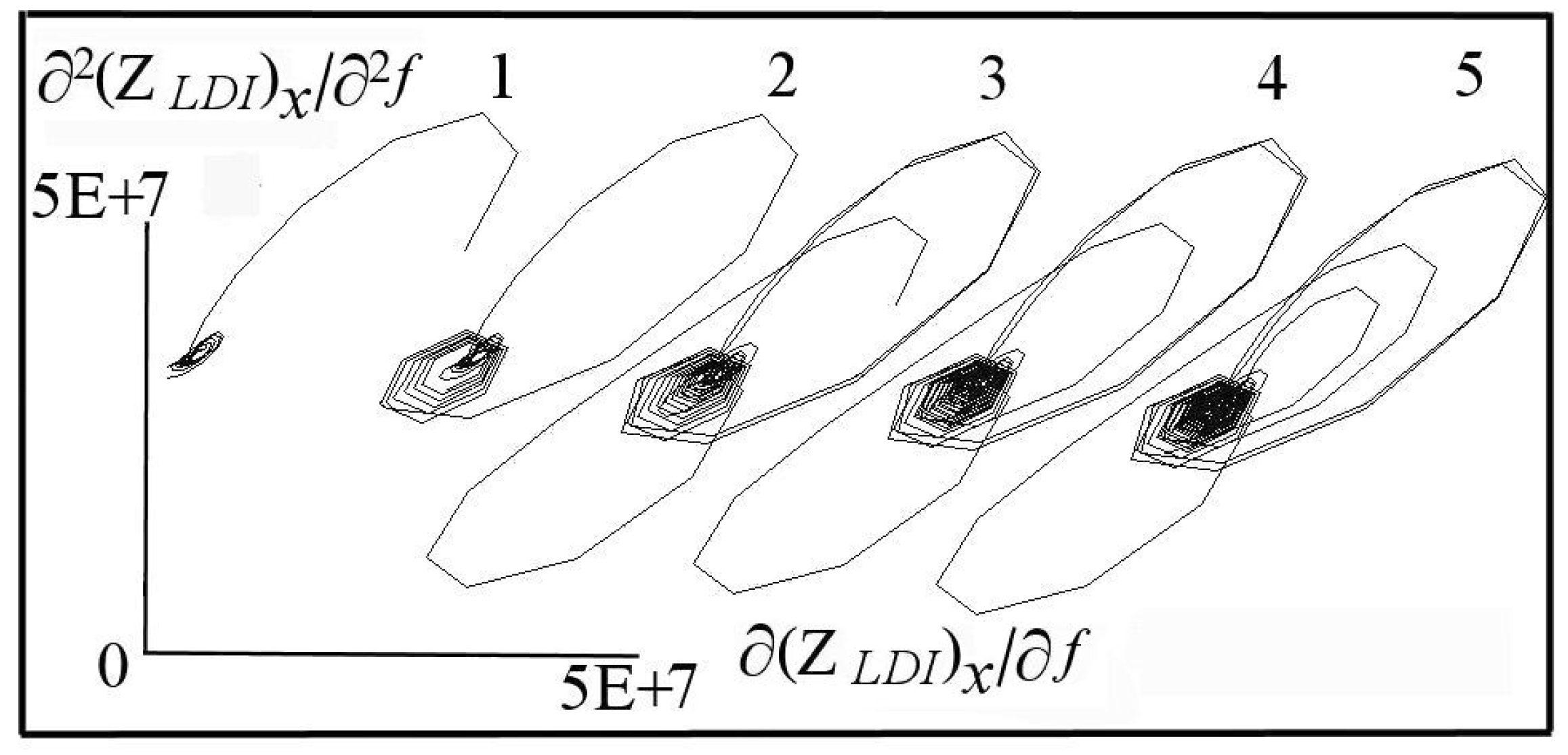
7.2.1. Aspects of Local Spectra at High Frequency

After presenting the results of chaos in peak A, the potential was moved between this peak and the shoulder (Figure 2(1)b). In this overlapping region, the scanning at high frequency would lead us to suspect capacitive and resistive events intervening on C₁, C₂, C₅ and R₁, R₂, R₅ (Figure 5 event 1 and Figure 19(1)). Figure 19(1) shows that amplitude produces regular decreasing resonance from E + 3 and an open-loop (graphs 2–3 event 5) at medium frequency. The electrochemical instability can be presumed to have been generated by the capacitive charge after pre-stability (Figure 19(1) event 1). It can be thought that event 1 corresponds to the electrolyte resistance. Figure 19(2,3) obtained for the phase-space derivative at high frequency shows that the trajectory suddenly diverges in event 2, where the local Lyapunov is 0.954. Then, the diverging trajectory converges forming a toroid in events 3 and 4. The local Lyapunov is −1.100, signifying instability followed by stability in the return spiraling when the Lyapunov exponent is negative. Eigenvalues are 1.07, −0.92 and 1.50.

7.2.2. Aspects of Local Spectra at Low Frequency

Figure 20(1) obtained for the local phase-space derivative at medium and low frequency represents the end of the previous toroid (event 2) after leaving the core at high frequency. At first glance, adsorbates arise from the rolling-up in the phase-space (event 2). Diverging scrolls begin at low frequency in event 6 from the first quarter, and propagate to other quarters. Diverging, scrolls in the $\partial Z_{{(LDI)}_{x,y}}/\partial f$ are associated with the transformation of adsorbates existing at different recovery rates. The evolution of adsorbates would take place through complexes. These complexes could change the stability of palladium charged in hydrogen. Change of strength would explain the signals obeying random mechanism (event 6). A significant signal leaving the core defines the feature of the elongated constant phase element going from −E + 1 to E + 4 (Figure 20(2) event 6) and obeys the Equations (6)–(11). Electrochemical chaos can produce different scrolls of repulsor according to the second model of adsorbed hydrogen acting from the toroid. This model 2 respects Equation (11) for the reversibility and the cathodic hydrogen complex charging (mechanism Heyrosky):

$${\left[{\mathrm{PdH}}_{\mathrm{k}}\right]}_{{\mathrm{ads}}_{(x)}}+\mathrm{n}{\mathrm{e}}^{-}\to {\left[{\mathrm{PdH}}_{\mathrm{k}}\right]}_{{\mathrm{ads}}_{(x,y)}}^{\mathrm{n}-}$$

(11)

Model 2 dominates when hydrogen adsorbate turns into a series of ${\left[{\mathrm{PdH}}_{\mathrm{k}}\right]}_{{\mathrm{ads}}_{(x,y)}}^{n-}$. Once the potential is high enough, Equation (6) falls, and Equation (11) takes over. ${\left[{\mathrm{PdH}}_{\mathrm{k}}\right]}_{ad{s}_{(x)}}$ can be considered the first surface attractor. Then, ${\left[{\mathrm{PdH}}_{\mathrm{k}}\right]}_{{\mathrm{ads}}_{(x,y)}}^{n-}$ is the second attractor where its electrical charge requires electrons again for electrochemical reaction. The adsorbate (x,y) is an intermediate of the species of x and y between peak A and the shoulder. In the presence of the two attractors, the electrochemical mechanism would oscillate before diffusion. Since absorbed hydrogen depends on the potential and the disturbance, hydrogen diffusing will also oscillate and strongly correlate. These events should be due to the combined action of these systems. The result will be a period-doubling chaos route if the adsorbates, either decreasing or increasing. In this condition, the Lyapunov exponent is synchronizing chaos where two systems are coupled so that there are driving and subordinate adsorptions. Therefore, the conditional response comes from the driving Equation (6) treated as simply the source of the chaotic master signal for diffusion.

Qualitatively, the convergence of the trajectory in phase-space with a regular decrease can be obtained from the variation of the capacitance at high frequency and the elongated constant phase element with or without the Warburg impedance at low frequency. Incorporating Equations (6) and (11) in the demonstration, Figure 19(2) proves that the variable ${\partial }^2{Z}_{{(LDI)}_{x,y}}/{\partial }^{2}f$ spirals around a converging point (events 1–4). Intrusion is going to the center of the closed-loop in the attractor. It is noticed that the converging point is responsible for connecting the symmetrical loops generated around the balanced model. However, as this state is stable and should provide one transient, the typical behavior is often characterized by a single period. In Figure 20, the spirals correspond to the resonant amplitude (event 2 in Figure 19). It can be seen an infinite trajectory (event 6) going beyond E + 4, called not-limited open-loop. This corresponds to ${\left[{\mathrm{PdH}}_{\mathrm{k}}\right]}_{{\mathrm{ads}}_{(x,y)}}^{n-}$ in Equations (2) and (3). The local Lyapunov value reported for the infinite trajectory is 1.441, signifying unstable open-loop for Equations (6) and (11). Therefore, in the model, there is a smooth action of the master precursor ${\left[{\mathrm{PdH}}_{\mathrm{k}}\right]}_{ad{s}_{(x)}}$ towards the subordinate system ${\left[{\mathrm{PdH}}_{\mathrm{k}}\right]}_{{\mathrm{ads}}_{(x,y)}}^{n-}$. When the ${\left[{\mathrm{PdH}}_{\mathrm{k}}\right]}_{ad{s}_{(x)}}$ acts, the system is a continuous dynamical system (Figure 19(3)) able to return until the initial point as an attractor in the phase-space forming a Silnikov orbit (E + 3). When the ${\left[{\mathrm{PdH}}_{\mathrm{k}}\right]}_{{\mathrm{ads}}_{(x,y)}}^{n-}$ is acting in Equation (11), the system is a discrete dynamical system (E + 1). The system can have two equilibria, which correspond to the two piecewise parts (x,y) of the palladium unsaturated in hydrogen. Stability can be examined by calculating the eigenvalues. The eigenvalues of the evolutionary operator determine the rate and character of the relaxation process. In this case, the equilibrium for the two conjugate complexes has two positive and one negative Eigenvalue (1.191, −0.094, and 1.403). These are in a relationship with the converging point making a global attractor whose decreasing spiraled signal is stable when it reaches zero. The diverging points in the scroll and the infinite trajectory not close (Figure 20(2) event 6) correspond to the positive eigenvalues. This can be more visible according to an equatorial projection. How can the effect of this trajectory be interpreted? This should sit by the constant phase element (CPE), and the Warburg impedance can be hidden by the two processes (x, y) [43].

7.2.3. Aspects of Power Spectra

Power spectra are a valuable signature for the dynamical systems derived from a sequential taking a run-frequency. When associated with a discrete Fourier transform signal, it is defined as the amplitude (${\mathrm{fd}}_{\mathrm{arb}}$). In considering the Equations (6)–(11), the spectrum at low frequency gives rise to the chaotic signal, whereas, at high-frequency, the signal should be stable. On this basis, the power spectrum combined with short segments provides a powerful tool for determinination of transients responsible for diverging chaos. The density of each segment is computed, and, when attached, they entail multiple transforms of the dynamical system in low frequency. This approach is amenable to efficient numerical computation in series showing two prominent peaks and a few tiny peaks for transients (Figure 21).

Therefore, power spectra are valuable for the dynamical system defined for short runs, and its approach is amenable to serial transform. The serial results plotted in Figure 21 show that it is possible to construct the chaotic dynamical systems according to the Lyapunov exponent of phase-space structure. In such a case, the Lyapunov exponent and power spectra are helpful for the determination of chaos. For this location, the peaks in the power spectra are 2 × 10⁻² Hz and 5 × 10⁻³ Hz. These correspond to the transients in Bode plot (Figure 9 and Equations (6)–(11)). Therefore, a reasonable reconstruction of chaos is obtained.

The Lyapunov exponent values indicate that the system is close to stability in the core at a medium frequency (−0.002), whereas, at low frequency, the system is unstable and diverges (0.326). In other words, the results of matrix Eigenvalues would indicate diverging points. These approaches would yield helpful ideas of chaotic dynamics. The EIS and voltammetry results are in good agreement with the chaos spectra that explicitly take into account the constant phase element and the blocking Warburg. Moreover, unstable measures on a chaotic attractor or repulsor involve analytical difficulties because it is generally not easy to obtain a stable distribution. After conducting a practical evaluation between the experimental data and the simulated model, the standard error is 0.0064, which is weak. The F-stat test is 142.48, and it assesses the correct sign for the results. The adjusted r-squared value is 0.8257, always a few less than the r-squared value of 0.8319. The fluctuating signal (full line), as shown in Figure 22(1), corresponds to a non-stationary state. The results of the autocorrelation function modifying the graph spatially act on the model (dashed line). The results are questionable for a range of 85% in confidence bound, while, for peak A, the confidence was 99%, but it remains acceptable examining the residuals (Figure 22(2)).

To illustrate such behavior, a simulation is performed to determine the variability between the tested values and those of the Fourier polynomial obtained from the power spectra. Approaches are incorporated into the calculation until equilibrium is reached between the two variables. The balance is presented in Figure 23, where the divergence coefficient (d) reflects the ratio of these two parameters. This distribution reveals a complex but very well-defined structure oriented in the positive or negative values regarding to the plane axes. This reflects the expansion of polynomial chaos for restricted diffusion in depth. Stability for the ratio d = 1 should match the diffusion, and disorder would be attributed to the adsorbed multi-transients in a disturbed area for d ≠ 1.

7.3. Measurements in the Equilibrium Potential

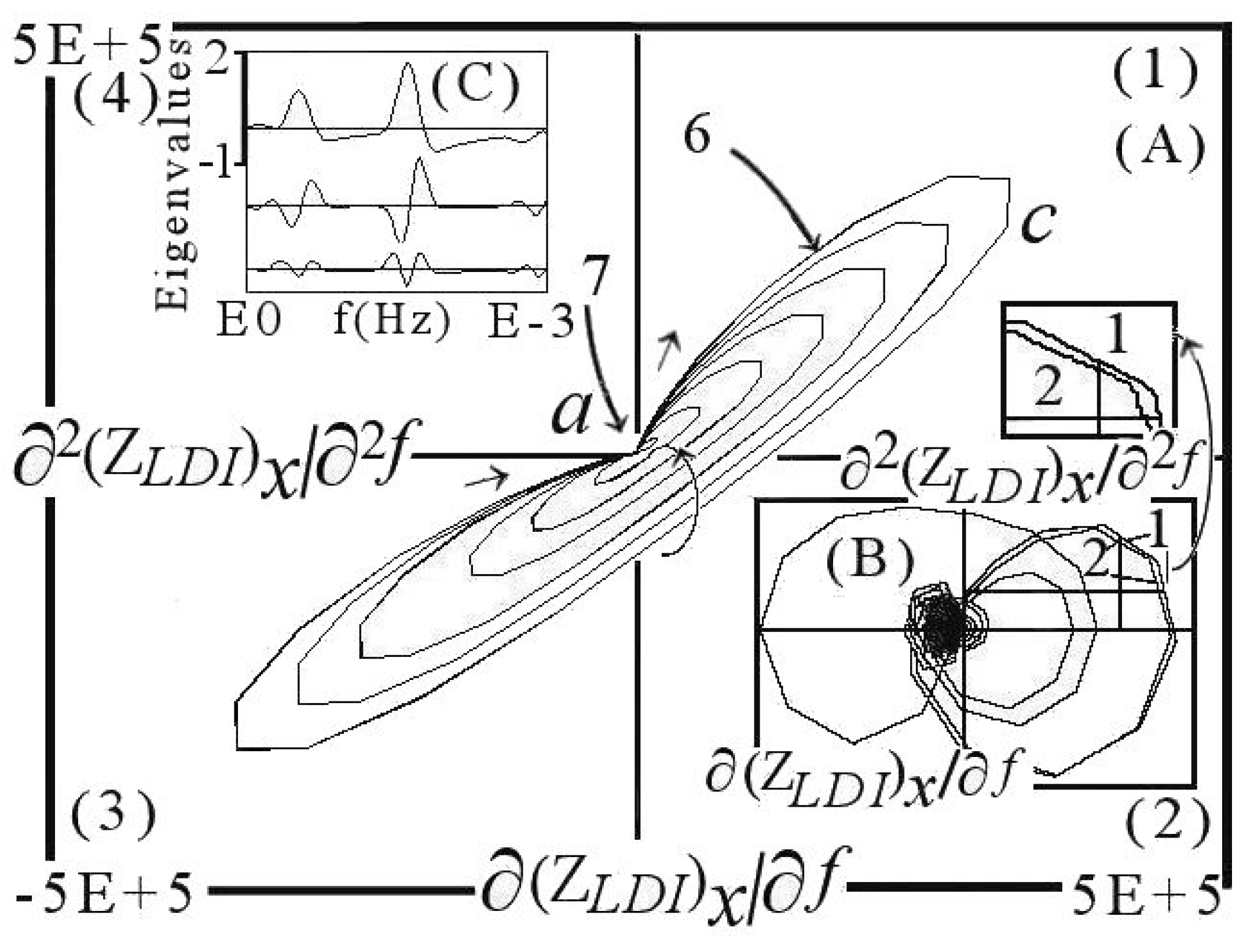
7.3.1. Aspects of Local Spectra

In addition to models 1–2 (Equations (6)–(11)), model 3 corresponds to the equilibrium between H_ads and O_ads according to the Tafel mechanism (Equations (12) and (13)). O_ads is formed regarding the high frequency’s charge transfer resistance. In the context of equilibrium potential for the interconnected cathodic and anodic multi-transients (Figure 6), the raw data represent oxidation of palladium associated with the adsorbed hydrogen (Equations (6)–(12), and Figure 24). Events 4 to 7 force the trajectory to oscillate and converge essentially into three-serial orbits as seen in Figure 25:

$${\left[{\mathrm{PdH}}_{\mathrm{k}}\right]}_{{\mathrm{ads}}_{(x,y)}}^{\mathrm{n}-}+(\mathrm{m}-\mathrm{n}){\mathrm{e}}^{-}\to {\left[{\mathrm{PdH}}_{\mathrm{k}}\right]}_{{\mathrm{ads}}_{(y)}}^{\mathrm{m}-}$$

(12)

$$2\mathrm{Pd}+{\mathrm{HO}}_2^{-}\to 2{\left[\mathrm{PdO}\right]}_{{\mathrm{ads}}_{(z)}}+{\mathrm{H}}^{+}+2{\mathrm{e}}^{-}$$

(13)

The process is not random, and this means that, for a given set of parameters, long-signals are repeated for an extensive range of frequency. Symmetric serial orbits in Figure 25 are a manifestation of hydrogen adsorbates where instabilities should be stabilized. The surface is acidified in the local region where palladium is oxidized, making it less stable (events 2–3). For basic information, according to Figure 2(1) (curve 1), the current attributed to the formation of adsorbed oxide corresponds to a lower recovery rate of 0.8. Consequently, superficial PdO electrochemically formed (z in Equation (4)) will not entirely block the hydrogen diffusion, unlike an oxidized palladium purifier for hydrogen isotope gas–gas.

It can be assumed that local acidification modifies the structure of the oxide capacitance (events 2–3) by breakdown, making it superficially semi-permeable to charge hydrogen. The higher frequency range corresponds to the electrolyte resistance (event 1). Instabilities are substantial for the high frequency (Figure 24 events 2–3) in the presence of oxidized palladium. At low frequency, adsorbed transients induce hydrogen diffusion. If volume compression or tensile strength and electrical field of adsorbates exceed a value for mechanical resistance of palladium, it can be expected that transients contribute to stress and chaos. Since absorbed hydrogen depends on the adsorption equilibrium with ${\left[\mathrm{PdO}\right]}_{ad{s}_{(z)}}$, hydrogen diffusing will oscillate and strongly correlate to balanced electrochemical reactions. Stress is considered nucleate in blocking superficial diffusion hardly visible in the Warburg impedance at a medium frequency (Figure 6). This is produced with subsequent instability in a deterministic mechanism (Figure 25(3) event 6).

Considering the electrical schema in Figure 4, the predominant combination related to this electrochemical system is the adsorption and absorption resistors combined with the capacitors and the Warburg impedances. In fact, ${\left[{\mathrm{PdH}}_{\mathrm{k}}\right]}_{{\mathrm{ads}}_{(y)}}^{m-}$ results from respective events cyclically reproducible using the rearrangement of three period routes in the chaotic orbit (Figure 26(2) event 6 and Figure 27(1) events 4, 5, 7). This proves that the derivative ${\partial }^2{Z}_{{(LDI)}_{x,y}}/{\partial }^{2}f$ has three orbits doubling routes making elliptical excursions with a jump (event 7) at low frequency for hydrogen blocking, and an orbit (event 6), ${\left[\mathrm{PdO}\right]}_{ad{s}_{(z)}}$, formed at high frequency. The orbits are lapped around the core, corresponding to the combined attractors. It is noticed that the converging point is responsible for connecting these symmetrical orbits generated around the equilibria of the three adsorbed modules (Equations (6), (11) and (12)). However, this state should be metastable and provide various transients. The boundary limit for an ordered behavior is often characterized by period-doubling through possible routes to chaos.

Oscillations are due to the nucleation of unstable species in the active region associated with the propagating stress and oxide breakdown. The initiation of superficial stress occurs only for a sufficient amount of hydrogen and perhydroxyl (Equation (13)). However, as the periodic oscillations decrease from E + 5 or are stable in the core (Figure 24), it should be a repair process at medium and low frequency (Figure 26 and Figure 27). Figure 26 and Figure 27 correspond to adsorption capacitance by oxygen (graph 1) and adsorption capacitance by hydrogen (graph 1). Therefore, it is interesting to examine the Lyapunov exponent. It varies positively between 0.021 and 1.26 for the different orbits. The lower values are placed near the “eye”. The eigenvalues for the tiny and prominent adsorbates are given in

Table 1. Variation of eigenvalues in a function of diversity of adsorbates.

Considered Adsorbates	Eigenvalues
3 dominant adsorbates (events 4, 5, 7)	0.983	−1.225	0.731
3 dominant + 1 tiny adsorbates	0.952	−1.328	1.045
3 dominant + 2 tiny adsorbates	0.911	−1.373	1.253
3 dominant + 3 tiny adsorbates	0.865	−1.382	1.393

. The eigenvalues measure the system’s complexity when the trajectory converges or diverges. Therefore, according to the results, the system can be in a stable or unstable configuration in the presence of tiny adsorbates, depending on the repair process. Nevertheless, to better discern the chaos, it is interesting to examine the intensity of the divergent random event 8. In Figure 24 and Figure 27, its positive value is E + 3. This is a weak value compared to that obtained for the blocking hydrogen at the reversible potential (5E + 7).

7.3.2. Aspects of Power Spectra

The low-frequency spectrum in Figure 28 can visualize dominant signals. These consist of three prominent peaks and tiny peaks corresponding to moderate transients. Using the power spectra, estimating the diffusion until hydrogen is blocked would be possible. Linearity was detected at high frequency, where the charge transfer resistance and the adsorption capacitance for hydrogen discharge intervene. However, these do not interfere with the complex signal. At low frequency, the complex impedance for blocking hydrogen diffusion also intervenes, so that short segment series at regular intervals were applied. This allows for estimating the chaos level directly in dominant frequencies. Therefore, low frequencies are designed to extract chaotic parts in the self-processes. Accordingly, the power spectra include a structural aspect acting on the phase-space. A vector deciding the trajectory governs the phase-space structure of a nonlinear dynamical system. Based on these observations, frequency analysis was compiled to study the local instability formed by transients. The advantage of this procedure is amenable to assemble the collected sectors, and this approach is relevant for any phase-space in blocking diffusion. Plotting the dominant frequency provides a representation of the global or local dynamics. This reveals that signal in the power frequency is of great interest to understand the diffusion type in non-regular or regular orbits. In particular, it appears that signal through the invariant core is of less importance than signal through orbit leading to diffusion and blocking diffusion. This is due to the overlapping hydrogen in chaotic palladium layers at low frequency. The equilibrium point in the core is stable for any initial value for high frequency.

From the phase-space, it can be seen that the chaotic behavior occurs in a Chua system. Chaotic dynamical systems of this type are invariably repulsive in low frequencies. A primary spectral peak dominates the signal at 2.5 mHz. The spectrum also contains two significant peaks at frequencies corresponding to interactions of transients at 6 and 40 mHz (as in Figure 16 and Figure 21). The three peaks correspond to the three transients: the primary and their combinations (Equations (6), (11) and (12)). These indicate coherence between voltammetry and dominant frequency in chaos spectra. Therefore, partial blocking diffusion is responsible for multi-signals. They constitute sufficient proof of the presence of chaos. Many other tiny peaks of sporadic dynamic signals are also revealed by frequency analysis. Such signals are evident even after careful and exhaustive removal. They could represent sub-transients with their chaos, and could be of fundamental importance to give valuable information on sub-dynamics. They would require more study through the energy concentration. The existence of a sub-event on a chaotic repulsor involves serious difficulties because it is generally difficult to obtain a stationary distribution. Dynamical systems in a chaotic regime fully reflect the properties of the attractor or repulsor.

The autocorrelation function can comfort results. Figure 29(1) shows the fluctuating signal corresponding to a non-stationary state at medium and low frequency. An algorithm using Fourier polynomial function was applied to detect these non-sub-stationary signals, thereby transient formation as in Equations (6)–(12). The goal of the Fourier process is also to predict the behavior of this physical model from a set of data. The equivalent noise in the series polynomial depends on the frequency. Fourier transform reveals distinct signatures ascribed to specific mechanisms distinguishing chaos. For that, Figure 29(1) endorses the results of the Fourier function modeled according to the residual error to quantify the deviation in the model [80]. This technique makes it possible to interpolate local variation of the computed model as a function of the neighboring experimental design points (full line). Combining the chaos technique with the Gaussian process (dashed line) makes it possible to capture the local variability. The values of the residuals are around 0.05, and these indicate that the model corresponds to the phase-state studied. Figure 29(2) illustrates the results for the modeling. The standard error is 0.049, which is weak. The F-stat test is 133.20, and it assesses the correct meaning for the results. The adjusted r-squared value is 0.8150, always a few less than the r-squared value of 0.8215. The adjusted r-squared increases only when the variable oxide is significant and affects the dependent variable of hydrogen. The 95% confidence bounds on the fitted values indicate that they are acceptably precise to predict chaos.

In Figure 30, the divergence coefficient according to the model and the Fourier transform at low frequency are determined. The d value compares the experimental response to the development of the chaos polynomial. Thus, when the ratio of these two parameters is d = 1, this indicates a perfect fit between the physical model and the chaos polynomial. When d is different than 1, it corresponds to instability. Applying Equation (10), a large part tends to d = 1, indicating the system’s stability. Considering the region where the d-test is different than the unity value, the hypothesis is in an unstable state and chaos is present in the local sector.

Consequently, in this system, there are the shared actions of the ${\left[\mathrm{PdH}\right]}_{ad{s}_{(x)}}$, ${\left[{\mathrm{PdH}}_{\mathrm{k}}\right]}_{{\mathrm{ads}}_{(x,y)}}^{n-}$, ${\left[{\mathrm{PdH}}_{\mathrm{k}}\right]}_{{\mathrm{ads}}_{(y)}}^{m-}$ and ${\left[\mathrm{PdO}\right]}_{ad{s}_{(z)}}$ on local diffusion, or for blocking double diffusion in low frequency as seen in electrochemical impedance spectroscopy (Figure 6). When the ${\left[{\mathrm{PdH}}_{\mathrm{k}}\right]}_{{\mathrm{ads}}_{(y)}}^{m-}$ is acting, the system is a continuous dynamical system returning until the initial point of the phase-space. When the ${\left[\mathrm{PdO}\right]}_{ad{s}_{(z)}}$ is operating, the system is a discrete dynamical system. The shape of the noise discriminates the presence of perhydroxyl radical. By decreasing the negative potential or increasing the presence of the perhydroxyl radical, the chaotic oscillation and stress increase.

8. Conclusions

This research was conducted to determine the limit of stress cracking by hydrogen or tritium in the palladium diffusion cathode. Regarding the experimental situation presenting the chaos, the character blocking diffusion coupled with instability is highlighted either in depth or in the subsurface of palladium cathode. This result can be interpreted from the interaction of complex transients formed on the entry surface facing electrolyte during diffusion or blocking diffusion. Obtaining the derivative of the phase space shows that the instability amplitude is most significant in the region of the reversible potential—then comes the region of the equilibrium potential and the region between them. Instabilities are most numerous on the bandwidth of frequencies at the reversible potential rather than other potentials. As a result, the region of reversible potential is most exposed to cracking corrosion. The complex formation develops the stress cracking in two front profiles of the cathodic membrane depending on the applied potential. Reversible potential leads to stress in depth, whereas equilibrium potential leads to stress in the subsurface. The development of electrochemical stress followed by repair depicts cyclic chaos coupled with pseudo-stability. This model has been validated, and, in the future, it will be interesting to examine the reversible and equilibrium potentials for the limiting diffusion for palladium alloys to know if they are less sensitive to stress corrosion cracking. It will also be useful to test the plasma electrolyzer for diffusion.

References

1. Conde, J.J.; Marono, M.; Sanchez-Hervas, J.M. Pd-based membranes for hydrogen separation: Review of alloying elements and their influence on membrane properties. Sep. Purif. Rev. 2017, 46, 152–177. [Google Scholar] [CrossRef]
2. Watanabe, N.; Yukawa, H.; Nambu, T.; Matsumoto, Y.; Zhang, G.X.; Morinaga, M. Alloying effects of Ru and W on the resistance to hydrogen embrittlement and hydrogen permeability of niobium. J. Alloys Compd. 2009, 477, 851–854. [Google Scholar] [CrossRef]
3. Lasser, R. Tritium and Helium-3 in Metals, Materials Science; Springer-Verlag Series in Materials Science: New York, NY, USA, 1989; Volume 9. [Google Scholar]
4. Tosti, S. Overview of Pd-based membranes for producing pure hydrogen and state of art at ENEA laboratories. Int. J. Hydrog. Energy 2010, 35, 12650–12659. [Google Scholar] [CrossRef]
5. Burkhanov, G.S.; Roshan, N.R.; Kolchugina, N.B.; Korenovsky, N.L.; Slovetsky, D.I.; Chistov, E. Palladium-based alloy membranes for separation of high-purity hydrogen from hydrogen containing gas mixtures. Platin. Met. 2011, 55, 3–12. [Google Scholar] [CrossRef]
6. Burkhanov, G.S.; Roshan, N.R.; Kol’chugina, N.B.; Korenovskii, N.L. Palladium rare-earth metal alloys-Advanced materials for hydrogen power engineering. Metal 2006, 15, 409–413. [Google Scholar]
7. Pozio, A.; de Francesco, M.; Jovanovica, Z.; Tosti, S. Pd-Ag hydrogen diffusion cathode for alkaline water electrolysers. Int. J. Hydrog. Energy 2011, 36, 5211–5217. [Google Scholar] [CrossRef]
8. Tosti, S.; Bettinali, L.; Violante, V. Rolled thin Pd and Pd-Ag membranes for hydrogen separation and production. Int. J. Hydrog. Energy 2000, 25, 319–325. [Google Scholar] [CrossRef]
9. Paolone, A.; Tosti, S.; Santucci, A.; Palumbo, O.; Trequattrini, F. Hydrogen and deuterium solubility in commercial Pd-Ag alloys for hydrogen purification. ChemEngineering 2017, 1, 14. [Google Scholar] [CrossRef] [Green Version]
10. Bellanger, S.; Rameau, J.J. Tritium recovery from tritiated water by electrolysis. Fusion Technol. 1999, 36, 296–308. [Google Scholar] [CrossRef]
11. Muranaka, T.; Shima, N. Improved electrolyzer for enrichment of tritium concentrations in environmental water samples. Fusion Sci. Technol. 2008, 54, 297–300. [Google Scholar] [CrossRef]
12. Bellanger, G. Changes of the breaking strain from content of tritium and cycling in a palladium cathode membrane. Fusion Eng. Des. 2011, 86, 357–362. [Google Scholar] [CrossRef]
13. Bellanger, G. Prospecting stress formed by hydrogen or isotope diffused in palladium alloy cathode. Materials 2018, 11, 2101. [Google Scholar] [CrossRef] [Green Version]
14. Thomas, J.; Hersbach, P.; Yanson, A.I.; Koper, M.T.M. Anisotropic etching of platinum electrodes at the onset of cathodic corrosion. Nat. Commun. 2016, 7, 12653. [Google Scholar] [CrossRef] [Green Version]
15. Yanson, A.I.; Antonov, P.V.; Rodriguez, P.; Koper, M.T.M. Influence of the electrolyte concentration on the size and shape of platinum nanoparticles synthesized by cathodic corrosion. Electrochim. Acta 2013, 112, 913–918. [Google Scholar] [CrossRef]
16. Ash, R.; Barrer, R.M. Diffusion with a concentration discontinuity: The hydrogen-palladium system. J. Phys. Chem. Solids 1960, 16, 246–252. [Google Scholar] [CrossRef]
17. Xia, D.; Song, S.; Wang, J.; Shi, J.; Bi, H.; Gao, Z. Determination of corrosion types from electrochemical noise by phase space reconstruction theory. Electrochem. Commun. 2012, 15, 88–92. [Google Scholar] [CrossRef]
18. Fernandez Macia, L.; Tourwe, E.; Pintelon, R.; Hubin, A. A new modeling method for determining electrochemical parameters from LSV experiments using the stochastic noise. Part I: Theory and validation. J. Electroanal. Chem. 2013, 690, 127–135. [Google Scholar] [CrossRef]
19. Astafev, E. The instrument for electrochemical noise measurement of chemical power sources. Rev. Sci. Instrum. 2019, 90. [Google Scholar] [CrossRef]
20. Rocha, P.R.F.; Schlett, P.; Kintzel, U.; Mailander, V.; Vandamme, L.K.J.; Zeck, G.; Gomes, H.L.; Biscarini, F.; de Leeuw, D.M. Electrochemical noise and impedance of Au electrode/electrolyte interfaces enabling extracellular detection of glioma cell populations. Nat. Sci. Rep. 2016, 6, 1–10. [Google Scholar] [CrossRef] [Green Version]
21. Curioni, M.; Monetta, T.; Bellucci, F. Modeling data acquisition during electrochemical noise measurements for corrosion studies. Corros. Rev. 2015, 33, 187–194. [Google Scholar] [CrossRef]
22. Jamali, S.S.; Zhao, Y.; Gao, Z.; Li, H.; Hee, A.C. In situ evaluation of corrosion damage using non-destructive electrochemical measurements. J. Ind. Eng. Chem. 2016, 43, 36–43. [Google Scholar] [CrossRef]
23. Jamali, S.S.; Mills, D.J.; Cottis, R.A.; Lan, T.Y. Analysis of electrochemical noise measurement on an organically coated metal. Prog. Org. Coatings 2016, 96, 52–57. [Google Scholar] [CrossRef] [Green Version]
24. Homborg, A.M.; Cottis, R.A.; Mol, J.M.C. An integrated approach in the time, Frequency and time-frequency domain for the identification of corrosion using electrochemical noise. Electrochim. Acta 2016, 222, 627–640. [Google Scholar] [CrossRef]
25. Homborg, A.M.; van Westing, E.P.M.; Tinga, T.; Ferrari, G.M.; Zhang, X.; de Wit, J.H.W.; Mol, J.M.C. Application of transient analysis using Hilbert spectra of electrochemical noise to the identification of corrosion inhibition. Electrochim. Acta 2014, 116, 355–365. [Google Scholar] [CrossRef]
26. Grafov, B.M. Theory of the first encounter with the boundary by a stochastic diffusion process in an equilibrium electrochemical RC-circuit. Russ. J. Electrochem. 2016, 52, 885–889. [Google Scholar] [CrossRef]
27. Grafov, B.M. The fractal theory of electrochemical diffusion noise: Correlations of the third and fourth order. Russ. Electrochem. 2016, 52, 220–225. [Google Scholar] [CrossRef]
28. Grafov, B.M. Fractal theory of electrochemical diffusion noise. Russian J. Electrochem. 2015, 51, 1–6. [Google Scholar] [CrossRef]
29. Banerjee, S.; Rondoni, L. Chaos, transport and diffusion—Applications of chaos and nonlinear dynamics in science and engineering. Springer Ser. 2015, 4, 31–63. [Google Scholar]
30. Garcia, E.; Hernandez, M.A.; Rodriguez, F.J.; Genesca, J.; Boerio, F.J. Oscillation and chaos in pitting corrosion of steel. Corrosion 2003, 59, 50–58. [Google Scholar] [CrossRef] [Green Version]
31. Wei, Y.-J.; Xia, D.-H.; Song, S.-Z. Detection of SCC of 304 NG stainless steel in an acidic NaCl solution using electrochemical noise based on chaos and wavelet analysis. Russ. Electrochem. 2016, 52, 560–575. [Google Scholar] [CrossRef]
32. Bahrami, M.J.; Hosseini, S.M.A.; Shahidi, M. Comparison of electrochemical current noise signals arising from symmetrical and asymmetrical electrodes made of Al alloys at different pH values using statistical and wavelet analysis. Part II: Alkaline solutions. Electrochim. Acta 2014, 148, 249–260. [Google Scholar] [CrossRef]
33. Ortiz Alonso, C.J.; Arely, L.G.M.; Hermoso-Diaz, I.A.; Chacon-Nava, J. Detection of sulfide stress cracking in a supermartensitic stainless steel by using electrochemical noise. Int. J. Electrochem. Sci. 2014, 9, 6717–6733. [Google Scholar]
34. Astafev, E.A.; Ukshe, A.E.; Dobrovolsky, Y.A. The model of electrochemical noise of a hydrogen-air fuel cell. J. Electrochem. Soc. 2018, 165, F604–F612. [Google Scholar] [CrossRef]
35. Astafev, E.A.; Ukshe, A. Flicker noise spectroscopy in the analysis of electrochemical noise of hydrogen-air PEM fuel cell during its degradation. Int. J. Electrochem. Sci. 2017, 12, 1742–1754. [Google Scholar] [CrossRef]
36. Lalik, E. Chaos in oscillatory sorption of hydrogen in palladium. J. Math. Chem 2014, 52, 2183–2196. [Google Scholar] [CrossRef] [Green Version]
37. Denissen, P.J.; Homborg, A.M.; Garcia, S.J. Interpreting electrochemical noise and monitoring local corrosion by means of highly resolved spatiotemporal real-time optics. J. Electrochem. Soc. 2019, 166, C3275–C3283. [Google Scholar] [CrossRef]
38. Zhang, Z.; Wu, X. Correlated pitting stages of 304 stainless steel with recurrence quantification analysis of electrochemical noise. Mater. Corros. 2019, 70, 197–205. [Google Scholar] [CrossRef]
39. Hou, Y.; Aldrich, C.; Lepkova, K.; Machuca, L.L.; Kinsella, B. Monitoring of carbon steel corrosion by use of electrochemical noise and recurrence quantification analysis. Corros. Sci. 2016, 112, 63–72. [Google Scholar] [CrossRef] [Green Version]
40. Huang, V.M.; Wu, S.-L.; Orazem, M.E.; Pebere, N.; Tribollet, B.; Vivier, V. Local electrochemical impedance spectroscopy: A review and some recent developments. Electrochim. Acta 2011, 56, 8048–8057. [Google Scholar] [CrossRef] [Green Version]
41. Yule, L.C.; Daviddi, E.; West, G.; Bentley, C.L.; Unwin, P.R. Surface microstructural controls on electrochemical hydrogen absorption at polycrystalline palladium. J. Electroanal. Chem. 2020, 872, 1–9. [Google Scholar] [CrossRef]
42. Bertocci, U.; Huet, F.; Nogueira, R.P.; Rousseau, P. Drift removal procedures in the analysis of electrochemical noise. Corrosion 2002, 58, 337–347. [Google Scholar] [CrossRef]
43. Leban, M.; Dolecek, V.; Legat, A. Electrochemical noise during non-stationary corrosion processes. Mater. Corros. 2001, 52, 418–425. [Google Scholar] [CrossRef]
44. Kearns, J.R.; Scully, J.R.; Roberge, P.R. Electrochemical Noise Measurement for Corrosion Applications; ASTM STP1277: Philadelphie, PA, USA, 1996. [Google Scholar]
45. Stringer, J.; Markworth, A.J. Applications of deterministic chaos theory to corrosion. Corros. Sci. 1993, 35, 751–760. [Google Scholar] [CrossRef]
46. Grafov, B.M. The Kramers-Moyal expansion for electrochemical stochastic diffusion. Russ. J. Electrochem. 2014, 50, 92–94. [Google Scholar] [CrossRef]
47. Rosenstein, M.T.; Collins, J.J.; De Luca, C.J. A practical method for calculating largest Lyapunov exponents from small data sets. Phys. D Nonlinear Phenom. 1993, 65, 117–134. [Google Scholar] [CrossRef]
48. Pecora, L.M.; Carroll, T.L.; Johnson, G.A.; Mar, D.J. Fundamentals of synchronization in chaotic systems, Concepts and applications. Chaos-Interdiscip. Nonlinear Sci. 1997, 7, 520–543. [Google Scholar] [CrossRef] [PubMed] [Green Version]
49. Zhdanov, V.P. Dynamics of surface diffusion. Surf. Sci. 1989, 214, 289–303. [Google Scholar] [CrossRef]
50. Sprott, J.C. Chaos and Time, Series Analysis; Oxford University Press: Oxford, UK, 2003. [Google Scholar]
51. Systat Software, Inc. TableCurve 2D, Automated Curve Fitting; Systat Publisher: Chicago, IL, USA, 2002. [Google Scholar]
52. Teong, S.P.; Li, X.; Zhang, Y. Hydrogen peroxide as an oxidant in biomass-to-chemical processes of industrial interest. Mater. Trans. 2019, 21, 5753–5780. [Google Scholar] [CrossRef]
53. Bellanger, G. Corrosion Induced by Low-Energy Radionuclides- Modeling of Tritium and Its Radiolytic and Decay Products Formed in Nuclear Installations, in Materials Science; Elsevier Science: Amsterdam, The Netherlands, 2004. [Google Scholar]
54. Okazaki, J.; Tanaka, D.A.P.; Tanco, M.A.L.; Wakui, Y.; Mizukami, F.; Suzuki, T.M. Hydrogren permeability study of the thin Pd-Ag alloy membranes in the temperature range across the α-β phase transition. J. Membr. Sci. 2006, 282, 370–374. [Google Scholar] [CrossRef]
55. Gabrielli, C.; Grand, P.; Perrot, H. Investigation of hydrogen adsorption and absorption in palladium thin films. J. Electrochem. Soc. 2004, 151, 1943–1949. [Google Scholar] [CrossRef]
56. Bosch, R.W.; Moons, F.; Zheng, J.H.; Bogaerts, W.F. Application of electrochemical impedance spectroscopy for monitoring stress corrosion cracking. Corrosion 2001, 57, 532–539. [Google Scholar] [CrossRef]
57. Zheng, C.; Yi, G. Investigating the influence of hydrogen on stress corrosion cracking of 2205 duplex stainless steel in sulfuric acid by electrochemical impedance spectroscopy. Corros. Rev. 2017, 35, 23–33. [Google Scholar] [CrossRef]
58. Zoltowski, P. Transport of hydrogen in elastic MHn solids. In Proceedings of the International Workshop—Materials to Systems, Berhampur, Odisha, India, 19–21 December 2017; pp. 16–22. [Google Scholar]
59. Tanaka, M. Electrochemical hydrogen pump using a high temperature type proton conductor under reduced pressure. J. Plasma Fusion Res. Series 2010, 9, 352–357. [Google Scholar] [CrossRef] [Green Version]
60. Bockris, J.O.M. On Hydrogen Damage and the Electrical Properties of Interfaces, In Stress Corrosion Cracking and Hydrogen Embrittlement of Iron Base Alloys; Nace Publishers: Houston, TX, USA, 1974. [Google Scholar]
61. Duncan, H.; Lasia, A. Mechanism of hydrogen adsorption/absorption at thin Pd layers on Au(111). Electrochim. Acta 2007, 52, 6195–6205. [Google Scholar] [CrossRef]
62. Lasia, A. Applications of the Electrochemical Impedance Spectroscopy to Hydrogen Adsorption, In Evolution and Absorption into Metals, Modern Aspects of Electrochemistry; Kluwer: New York, NY, USA, 2002; Volume 35, pp. 1–49. [Google Scholar]
63. Jacobsen, T.; West, K. Diffusion impedance in planar, cylindrical and spherical symmetry. Electrochim. Acta 1995, 40, 255–262. [Google Scholar] [CrossRef]
64. Scully, J.R. Electrochemical Impedance—Analysis and Interpretation; STP1188—ASTM: Philadelphia, PA, USA, 1993. [Google Scholar]
65. Anishchenko, V.S.; Astakhov, V.; Vadivasova, T.; Neiman, A. Nonlinear Dynamics of Chaotic and Stochastic Systems— Tutorial and modern Developments; Springer: New York, NY, USA, 2007. [Google Scholar]
66. Muthuswamy, B. Implementing memristor based chaotic circuits. Int. J. Bifurc. Chaos 2010, 20, 1335–1350. [Google Scholar] [CrossRef]
67. Cottis, R.; Turgoose, S.; NACE International. Electrochemical Impedance and Noise; Corrosion Testing Made Easy, Nace: Houston, TX, USA, 1999. [Google Scholar]
68. Zhong, G.-Q.; Ayrom, F. Periodicity and chaos circuit. Trans. Circuits 1985, 32, 501–503. [Google Scholar] [CrossRef]
69. Chua, L.O.; Lin, G.-n. Intermittency in a piecewise-linear circuit. IEEE Trans. Circuits Syst. 1991, 38, 510–520. [Google Scholar] [CrossRef]
70. Bartissol, P.; Chua, L.O. The double hook. IEEE Trans. Circuits Syst. 1988, 35, 1512–1522. [Google Scholar] [CrossRef]
71. Wigdorowitz, B.; Petrick, M.H. Modelling concepts arising from an investigation into a chaotic system. Mathl. Comput. Model. 1991, 15, 1–16. [Google Scholar] [CrossRef] [Green Version]
72. Madan, R.N. Chua Circuit—A Paradigm for Chaos, World Scientic; Non-Linear Science, Rabinder: Madan, Bulgaria, 1993. [Google Scholar]
73. Bellanger, G.; Rameau, J.J. Determination of tritium adsorption and diffusion parameters in a palladium-silver alloy by electrochemical impedance analysis. Fusion Technol. 1997, 32, 94–106. [Google Scholar] [CrossRef]
74. Chua, L.O.; Lin, G.-N. Canonical realization of Chua circuit family. IEEE Trans. Circuits Syst. 1990, 37, 885–902. [Google Scholar] [CrossRef] [Green Version]
75. Limphodaen, N.; Chansangiam, P. Mathematical analysis for classical Chua circuit with two nonlinear resistors. Songklanakarin J. Sci. Technol. 2020, 42, 678–687. [Google Scholar] [CrossRef]
76. Cheng, W.; Luo, S.; Chen, Y. Use of EIS, Polarization and electrochemical noise measurements to monitor the copper corrosion in chloride media at different temperatures. Int. J. Electrochem. Sci. 2019, 14, 4254–4263. [Google Scholar] [CrossRef]
77. Anishchenko, V.S.; Vadivasova, T.E.; Okrokvertskhov, G.A.; Strelkova, G.I. Correlation analysis of dynamical chaos. Phys. A 2003, 325, 199–212. [Google Scholar] [CrossRef]
78. Le Maitre, O.P.; Reagan, M.T.; Najm, H.N.; Ghanem, R.G.; Knio, O.M. A stochastic projection method for fluid flow. ii. Random process. J. Comp. Phys. 2002, 181, 9–44. [Google Scholar] [CrossRef] [Green Version]
79. MaItre, O.P.L.; Knio, O.M.; Najm, H.N.; Ghanem, R.G. A stochastic projection method for fluid flow. i. Basic formulation. J. Comp. Phys. 2001, 173, 481–511. [Google Scholar] [CrossRef] [Green Version]
80. Blatman, G.; Sudret, B. Adaptive sparse polynomial chaos expansion based on least angle regression. J. Comput Phys 2011, 230, 2345–2367. [Google Scholar] [CrossRef]
Figure 1. Electrolyzer for hydrogen production. (A): schematic of electrolyzer; (B): prototype electrolyzer; (C): schematic of Pd cathode membrane with hydrogen diffusion. 1: tank for water; 2: circulation pump; 3: water circulation piping; 4: electrolyzer; 5: water compartment; 6: hydrogen compartment; 7: anode; 8: palladium cathode membrane; 9: hydrogen extraction; 10: oxygen extraction. ads: adsorption, ins: insertion.
Hydrogen 03 00010 g001
Figure 2. (1) Voltammetry plot examining the E rev and E eq potentials for palladium charged in hydrogen. Surface area: 0.1 cm2, temperature: 20 °C, NaOH: 0.1 mol dm−3, scan rate: 200 mV s−1, cathodic scan limits: (1) 0 V, (2) −0.85 and (3) −1.15 V/NHE, time charging hydrogen τ : 5 s. In window (2): A(a): on peak A, position a; B(b): between peak A and shoulder B, position b; B(c): on shoulder B, position c. Tiny peaks are small intermediate transients.
Hydrogen 03 00010 g002
Figure 3. (1): Nyquist diagram for palladium charged in hydrogen. Applied potential: −0.35 V/NHE, position towards reversible potential, LD: hydrogen blocking; (2): 3D contour graph, real impedance and frequency (f) in X–Z axes (lateral), imaginary impedance in dragging the y-axis (vertical).
Hydrogen 03 00010 g003
Figure 4. Equivalent electrical circuit for hydrogen diffusion and blocked hydrogen. Rel: electrolyte resistance, Rct: charge transfer resistance, Rdl: double-layer capacitance, R1,2,5: adsorption-transfer charge resistances, C1,2: adsorption capacitances, R3,4: insertion resistances, R1,2: diffusion impedances, arrows showing the compressive and expansive stress, (1): primary diffusion (reversible potential), (2): secondary diffusion (equilibrium potential) respectively in (a,b) for transient impedance.
Hydrogen 03 00010 g004
Figure 5. Nyquist diagram for palladium charged in hydrogen. Applied potential between peak A and shoulder.
Hydrogen 03 00010 g005
Figure 6. Nyquist diagram for palladium charged in hydrogen. Applied potential at potential between shoulder B and equilibrium potential, position c.
Hydrogen 03 00010 g006
Figure 7. View of cracks, (a): cracks near blocking entry surface facing to electrolyte; (b): cracks crossing right through thickness of palladium; (c): cracks near blocking exit surface, arrow showing cracks, arrow showing direction of penetration for hydrogen—scaling is indicated in the photograph.
Hydrogen 03 00010 g007
Figure 8. Influence of cathodic current on permeability, (A): near reversible potential for hydrogen launching in deep penetration; (B): near equilibrium potential in subsurface with palladium oxidation.
Hydrogen 03 00010 g008
Figure 9. Reversed Bode spectrum corresponding to two characteristic Warburg behavior ( f c ( 1 , 2 ) ), (1): on impedance; (2): on θ phase-angle at low frequency (ellipse) in an active region with hydrogen blocking (LD).
Hydrogen 03 00010 g009
Figure 10. Instability events for impedance of palladium–hydrogen complex at potential in peak A. Views (1): −0.25 V/NHE, (2): −0.31 V/NHE, (3): −0.37 V/NHE, (4): −0.45 V/NHE.
Hydrogen 03 00010 g010
Figure 11. Phase-space derivative on the diverging loops and converging spirals (events 5–8) in the region of peak A. Views (13).
Hydrogen 03 00010 g011
Figure 12. (A): Phase-space derivative at low frequency in converging spirals (event 6) for region of voltammetry peak A; (B) example of a graph to select vectors (Figure 11 event 5) for determination of Lyapunov exponent in the upper right quarter, same scaling; (C) eigenvalues at low-frequency scale.
Hydrogen 03 00010 g012
Figure 13. Phase-space derivative at medium frequency in diverging open-loop (events 3-4-5-9) for region of peak A.
Hydrogen 03 00010 g013
Figure 14. Phase-space derivative for diverging (events 3–5) and converging (event 8) loops in leaving funnel (event 6) in a region of peak A at a different viewing angle. Views (1,2).
Hydrogen 03 00010 g014
Figure 15. Series of disorderly episodes for convergence and divergence from Figure 14(2). Loops running (1–5).
Hydrogen 03 00010 g015
Figure 16. Power spectra and dominant frequency for Warburg impedance at reversible potential. a: 2.5 mHz.
Hydrogen 03 00010 g016
Figure 17. Fourier series polynomial. Envelope of autocorrelation function at reversible potential. Graph (1): autocorrelation function φ , 1,2: overlapped variation of experimental curve and computed model; graph (2): residual deviation σ .
Hydrogen 03 00010 g017
Figure 18. d divergence coefficient and chaos at peak A.
Hydrogen 03 00010 g018
Figure 19. (1): Instability depending on impedance between peak A and shoulder B; (2,3): phase-space at high frequency for closed spiral and open-route at different viewing angles.
Hydrogen 03 00010 g019
Figure 20. Phase-space for trajectory at low frequency and in different orientation (1,2) for potential between peak A and shoulder B.
Hydrogen 03 00010 g020
Figure 21. Power spectra and dominant frequency for Warburg impedance between equilibrium and reversible potential. a: 5 × 10⁻³ Hz, b: 2 × 10⁻² Hz.
Hydrogen 03 00010 g021
Figure 22. Fourier series polynomial. Envelope of autocorrelation function between equilibrium and reversible potential. Graph (1): autocorrelation function φ , 1: variation of experimental curve (full line), 2: variation of computed model (dashed line); graph (2): residual deviation σ .
Hydrogen 03 00010 g022
Figure 23. d divergence coefficient and chaos between peak A and equilibrium potential.
Hydrogen 03 00010 g023
Figure 24. Unstable events decreasing with several steps in palladium impedance at equilibrium potential.
Hydrogen 03 00010 g024
Figure 25. Phase-space at equilibrium potential. (1): front view; (2): angular view; (3): side view. Closed three-scrolls in combined repulsors (events 4–5) and attractors (events 2–3), a jump (event 7), and open-route (event 6).
Hydrogen 03 00010 g025
Figure 26. Phase-space at equilibrium potential for two first episodes at high frequency in Figure 24. (1): oxide adsorption; (2): oxide rearrangement.
Hydrogen 03 00010 g026
Figure 27. Phase-space at equilibrium potential at low frequency in Figure 24. (1): hydrogen adsorption, events 4 to 7; (2): partial projection, and changing perspective view for unstable event 8 in Figure 24.
Hydrogen 03 00010 g027
Figure 28. Power spectra and dominant frequency for Warburg impedance at equilibrium potential. a: 2.5 mHz, b: 6 mHz, c: 40 mHz.
Hydrogen 03 00010 g028
Figure 29. Fourier series polynomial. Envelope of autocorrelation function at equilibrium potential. Graph (1): autocorrelation function φ , 1: variation of experimental curve (full line); 2: variation of computed model (dashed line); graph (2): residual deviation σ .
Hydrogen 03 00010 g029
Figure 30. d divergence coefficient and chaos at equilibrium potential.
Hydrogen 03 00010 g030