
Self-Directed Mobile Robot Navigation Based on Functional Firefly Algorithm (FFA)


Abstract
:1. Introduction
2. Review of Literature
- Fireflies are unisex, but their attraction is based on intensity rather than gender;
- The attraction is proportional to brightness, from lesser brightness to greater brightness;
- The brightness interacts with the landscape of the objective function.
3. Proposed Functional Firefly Algorithm
| Algorithm 1 Fuctional Firefly (FFA). |
| #Function FunctionalFireflyAlgorithm(): Initialize robot navigation Initialize the population of fireflies Initialize the objective function Initialize light intensity of fireflies (I) Initialize absorption coefficient Initialize the distance between two fireflies (r) Vary attractiveness Classify fireflies into two groups based on intensity: , l: less intensity. , h: high intensity. t = 0 maxiterations = max(Xλ) While # Update lowintensity fireflies For i in Xλl: If ; ; If : If ; ; If If # Calculate the objective function # Update fireflies based on the objective function t = t + 1 # Optimized f(λ) Optimized function f(λ) End robot navigation |
4. Simulation and Experimental Result Analysis
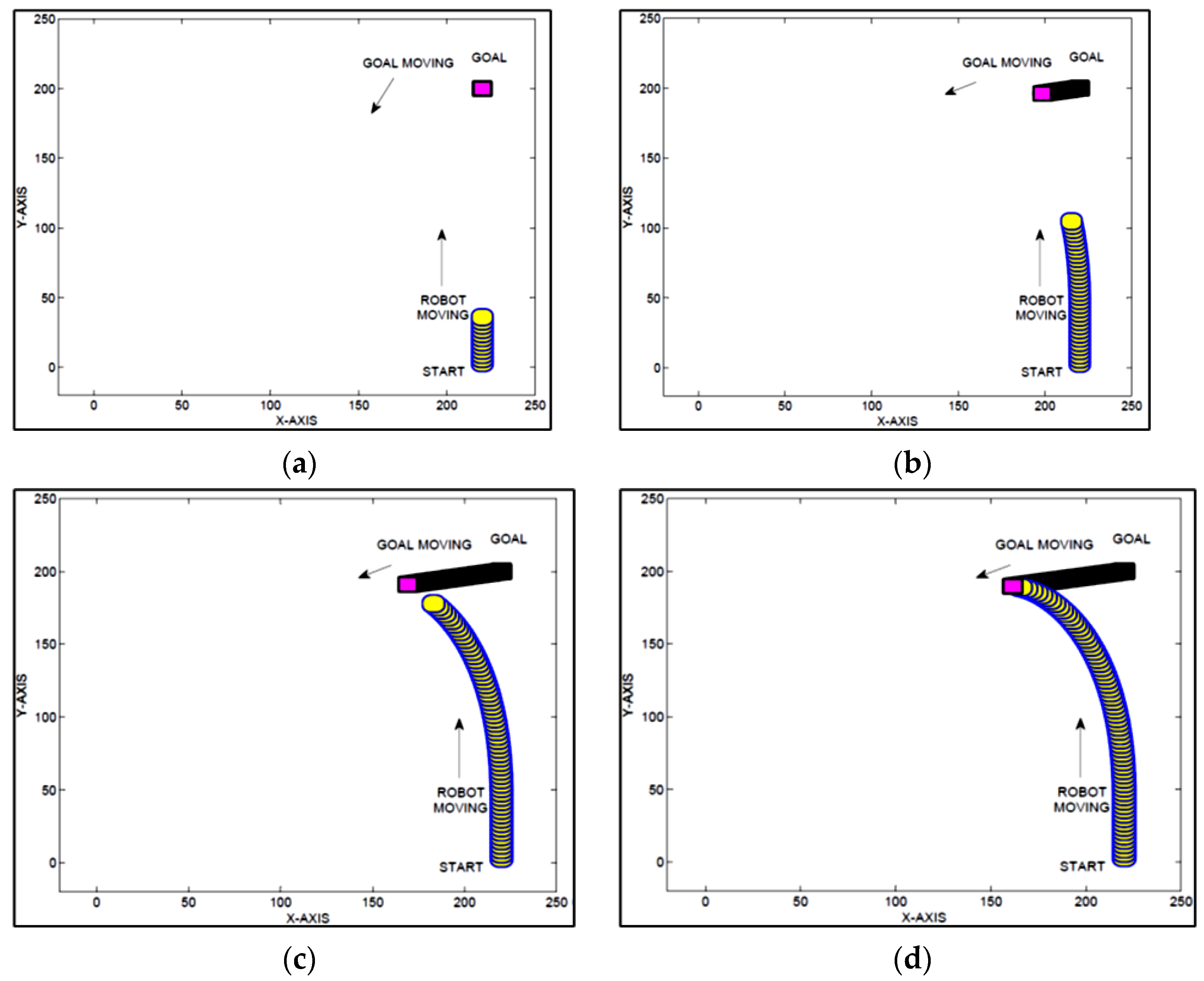
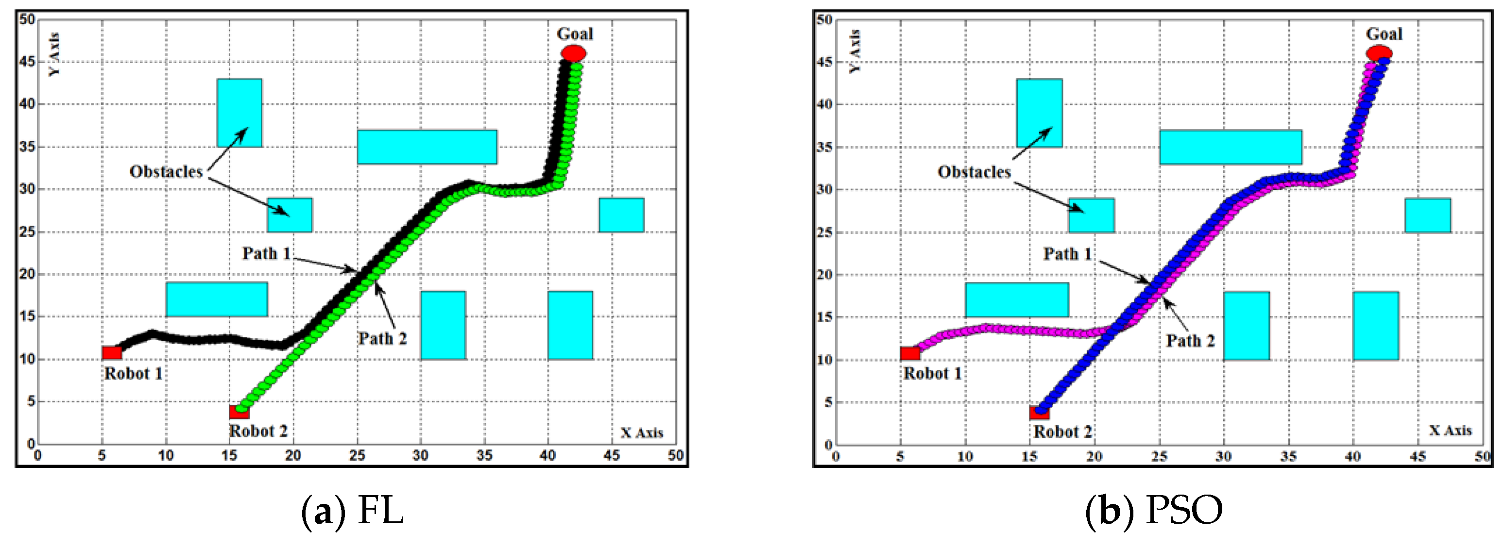
4.1. Mobile Robot Navigation Simulation Results
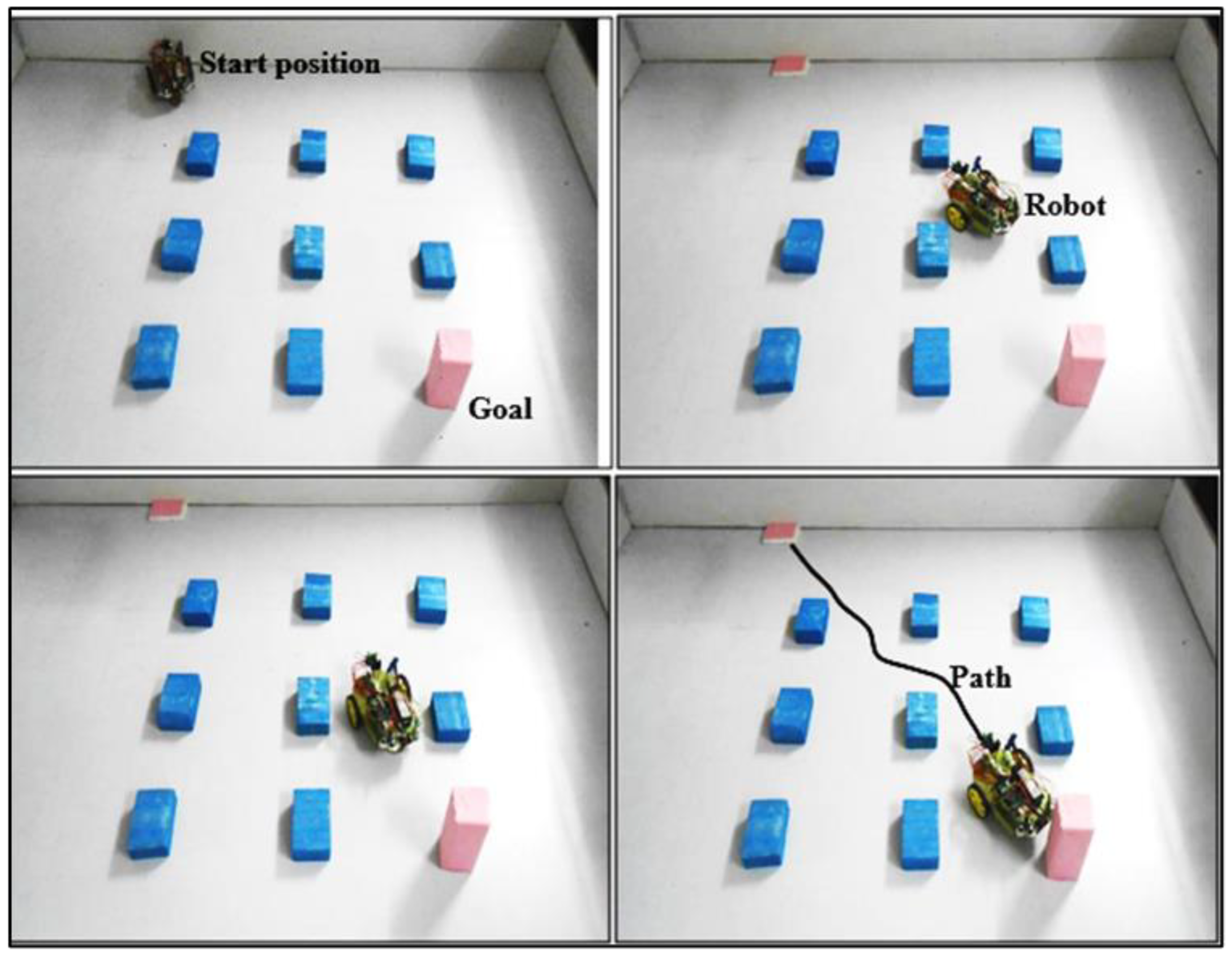
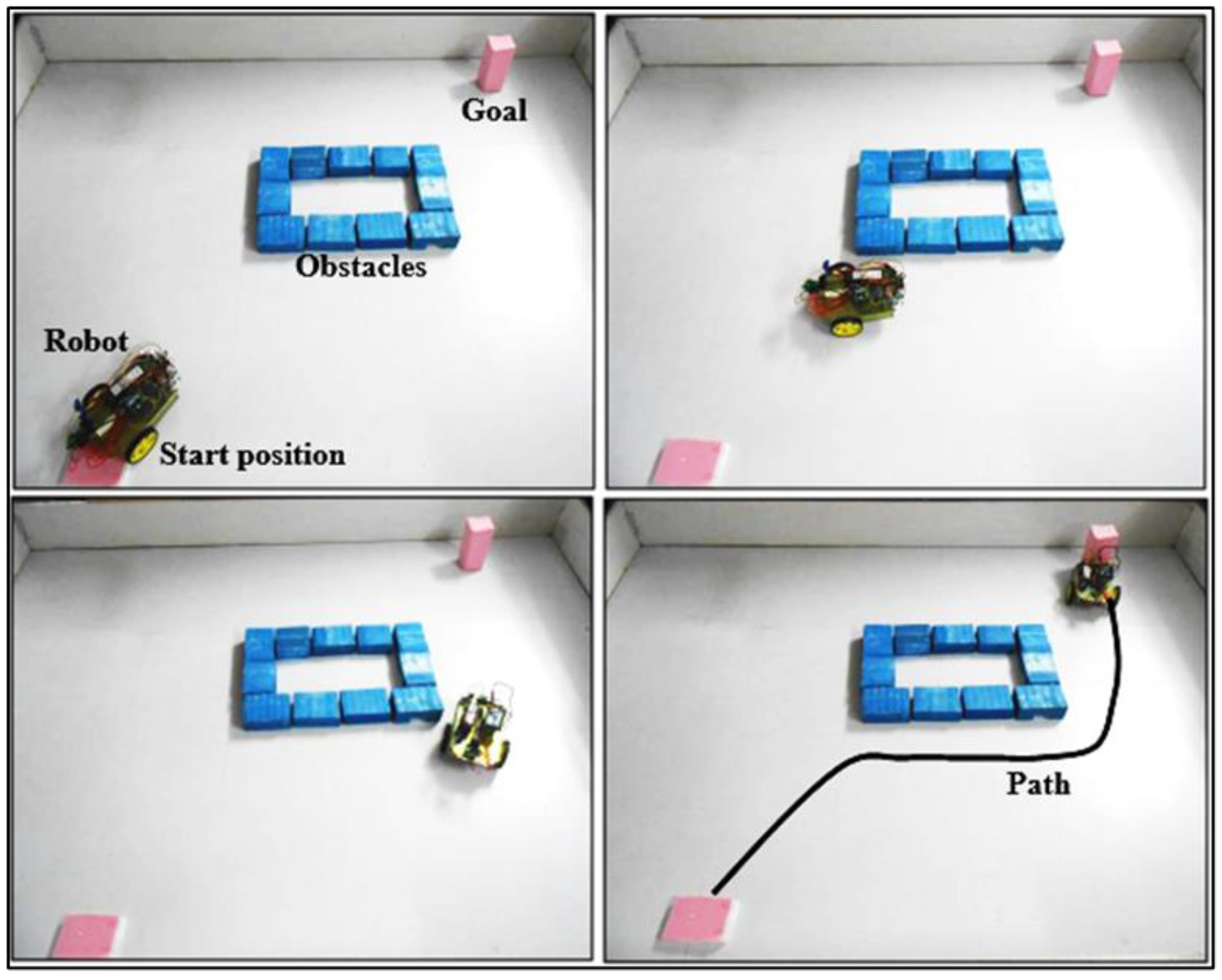
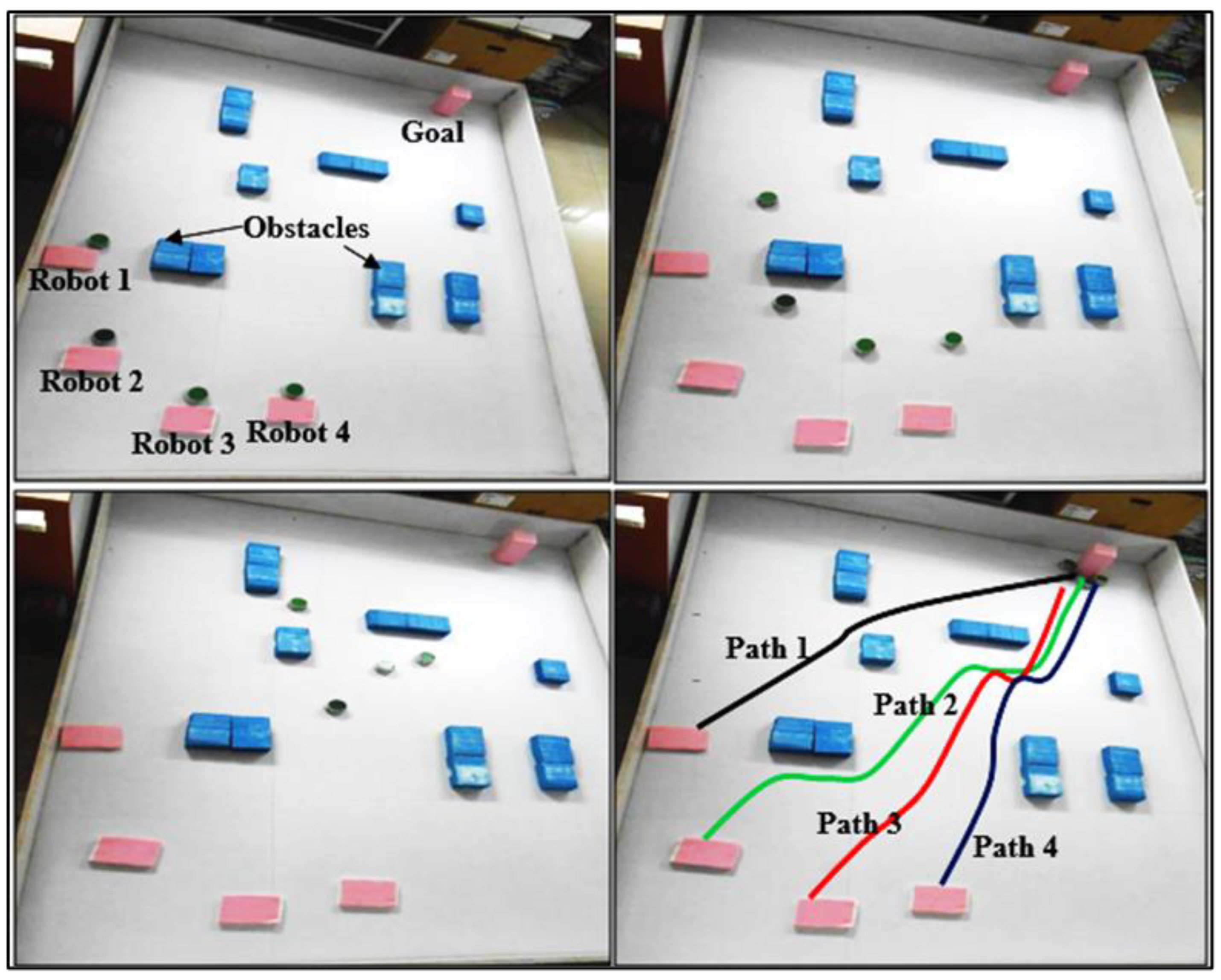
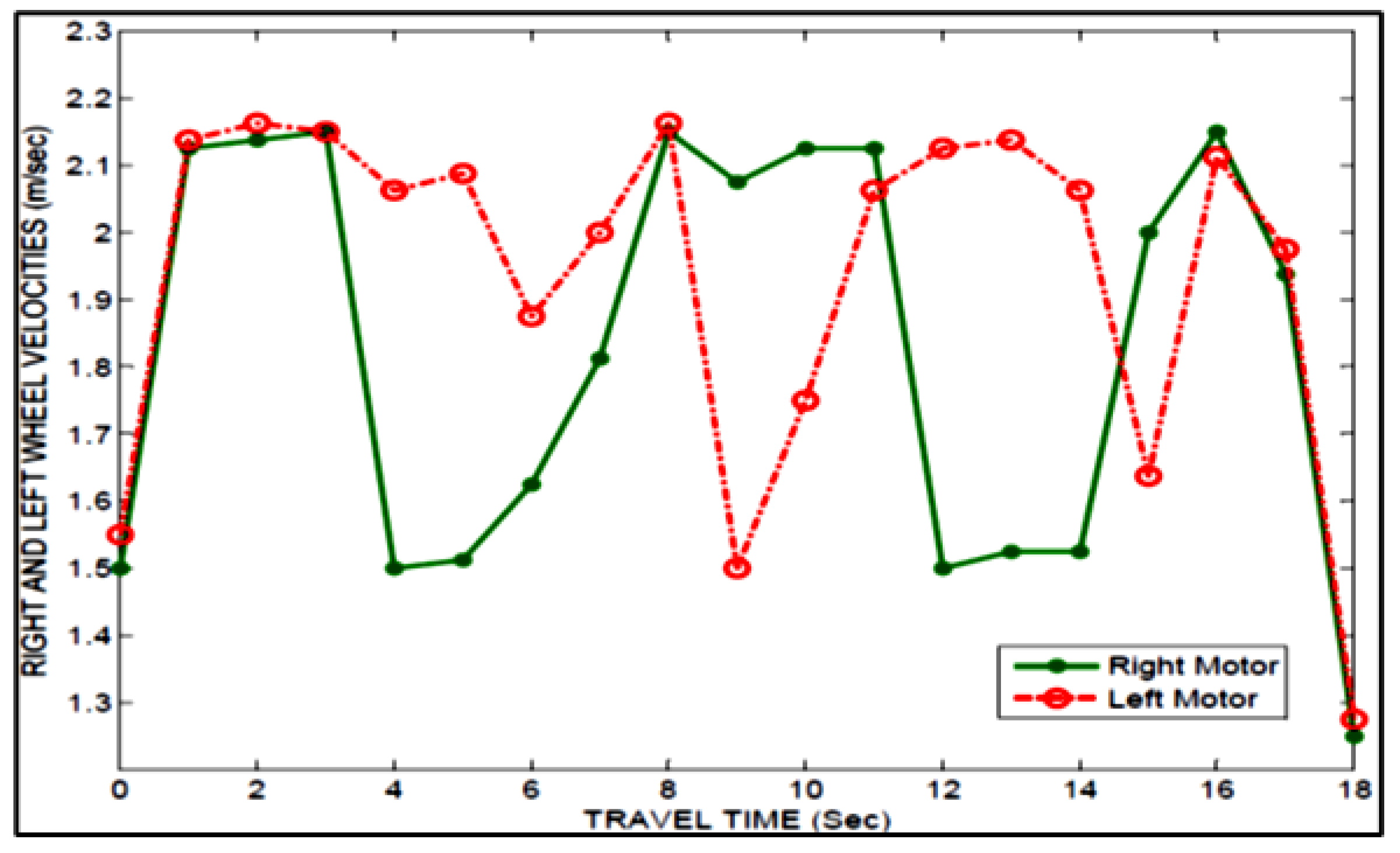
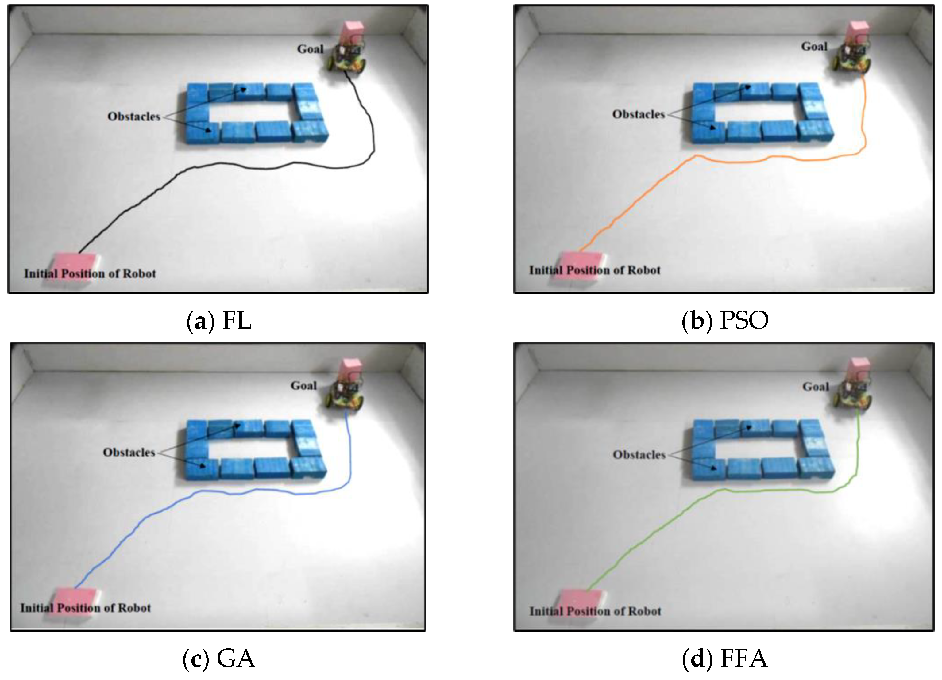
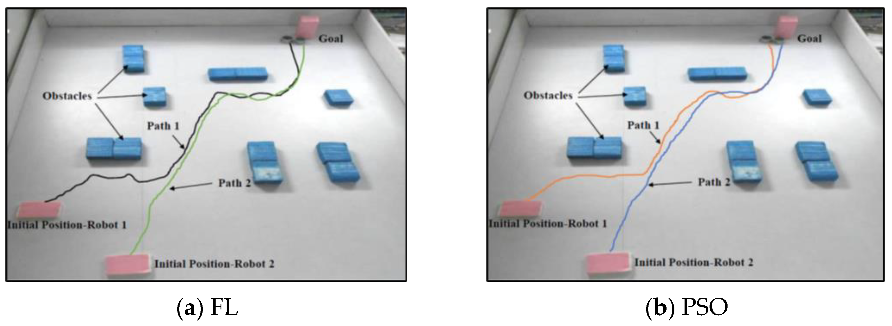
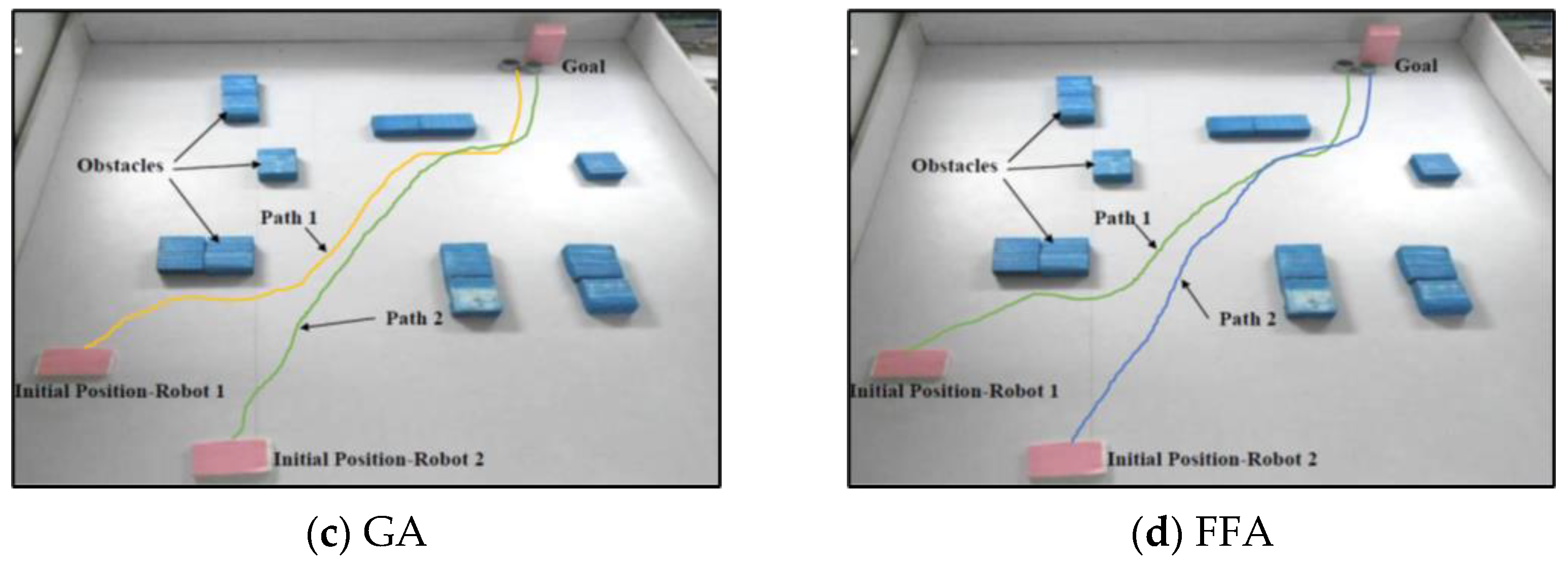
4.2. Mobile Robot Navigation Experimental Results
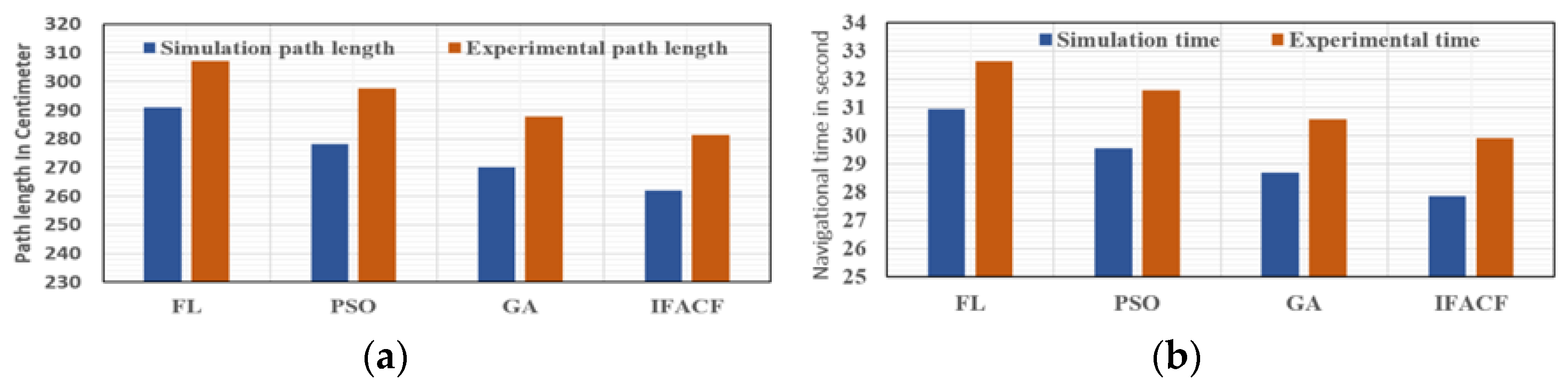
4.3. Comparative Analysis of Experimental vs. Simulation
4.4. Proposed FFA Controller versus Another Intelligent Controller over the Same Environmental Setup

| Sl. No. | Name of Controllers | Simulation Path Length (cm) | Simulation Time (s) | Real-Time Path Length (cm) | Real-Time (s) |
|---|---|---|---|---|---|
| 1 | FL | 291.06 | 30.93 | 307.23 | 32.65 |
| 2 | PSO | 278.12 | 29.55 | 297.528 | 31.62 |
| 3 | GA | 270.03 | 28.69 | 287.82 | 30.58 |
| 4 | FFA | 261.97 | 27.84 | 281.35 | 29.90 |
| Sl. No. | Name of Controllers | Simulation Path Length (cm) | Simulation Time (s) | Real-Time Path Length (cm) | Real-Time (s) | |
|---|---|---|---|---|---|---|
| 1 | FL | Robot-1 | 245.78 | 26.12 | 252.2 | 26.802 |
| Robot-2 | 213.44 | 22.68 | 226.38 | 24.05 | ||
| 2 | PSO | Robot-1 | 239.08 | 25.40 | 247.08 | 26.25 |
| Robot-2 | 210.50 | 22.37 | 216.67 | 23.02 | ||
| 3 | GA | Robot-1 | 229.61 | 24.40 | 232.84 | 24.74 |
| Robot-2 | 207.21 | 22.02 | 210.21 | 22.34 | ||
| 4 | FFA | Robot-1 | 223.14 | 23.71 | 230.38 | 24.48 |
| Robot-2 | 205.97 | 21.89 | 208.74 | 22.18 | ||
| Sl. No. | Name of Controllers | Simulation Path Length (cm) | Simulation Time (s) |
|---|---|---|---|
| 1 | FL | 244.55 | 26 |
| 2 | PSO | 237.69 | 25.62 |
| 3 | GA | 232.84 | 24.74 |
| 4 | FFA | 228.76 | 23.87 |
| Sl. No. | Name of Controllers | Simulation Path Length (cm) | Simulation Time (s) |
|---|---|---|---|
| 1 | FL | 161.70 | 17.18 |
| 2 | PSO | 153.61 | 16.32 |
| 3 | GA | 142.90 | 15.18 |
| 4 | FFA | 139.29 | 14.80 |


4.5. Proposed FFA Controller versus Published Work

5. Conclusions
Author Contributions
Funding
Institutional Review Board Statement
Informed Consent Statement
Data Availability Statement
Conflicts of Interest
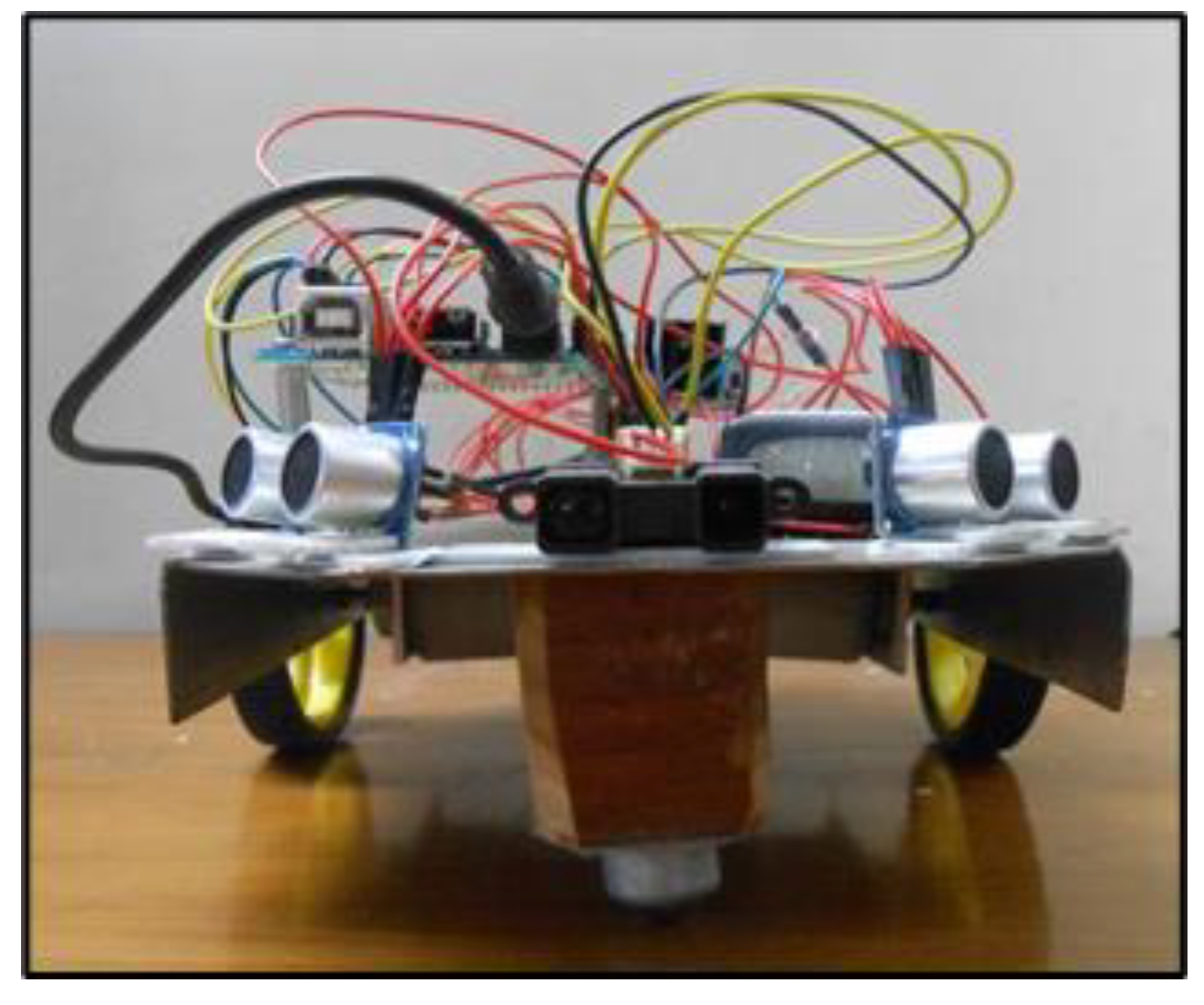
Appendix A
| Elements | Technical Specification | |
|---|---|---|
| 1 | Processor | ATmega2560 (Arduino Mega 2560, Arduino UNO, Olatus Systems, Guwahati, India) |
| 2 | RAM | 8 KB, EEROM-4 KB |
| 3 | Flash | 256 KB (8 KB used for boot loader) |
| 4 | Motors | 2-DC gear motors with incremental encoders |
| 5 | Distance sensors | (a) Infrared sensors with up to 150 cm range (b) Ultrasonic sensors with up to 400 cm range |
| 6 | Speed | Max: 0.47 m/s, Min: 0.03 m/s |
| 7 | Power | Power adapter or Rechargeable NiMH Battery (2000 mAh) |
| 8 | Communication | USB connection to the computer |
| 9 | Size | Length: 25 cm, Width: 19 cm, Height: 12 cm |
| 10 | Weight | Approx. 1100 g |
| 11 | Payload | Approx. 4000 g |
| 12 | Remote control Software via USB cable | C/C++17 ® (on PC, MAC OS 12) MATLAB R2021a ® (on PC, MAC OS 12, Linux) |
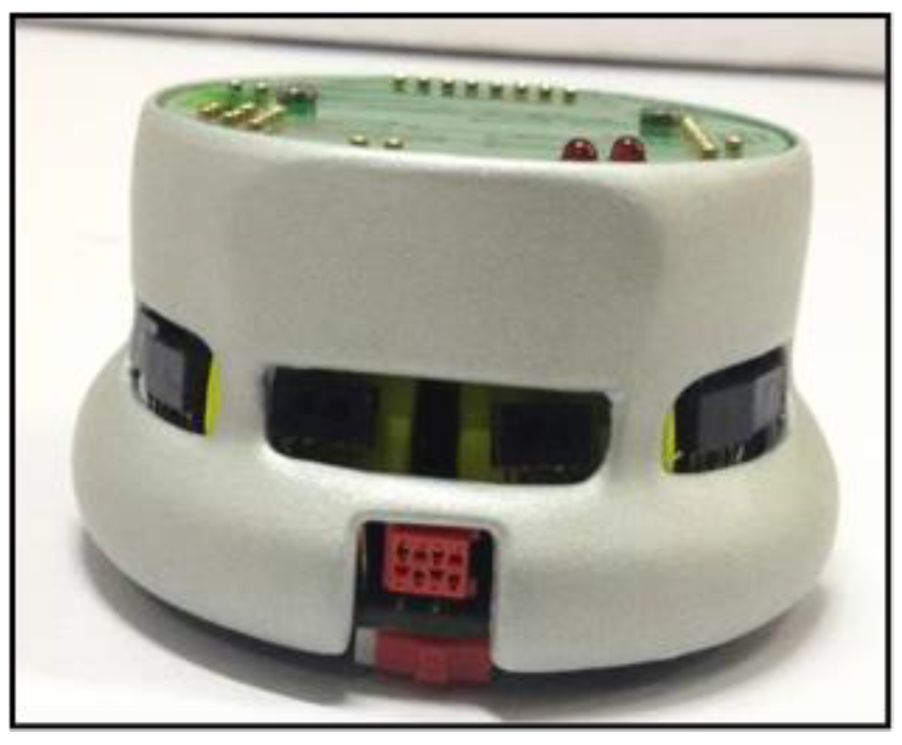
| Elements | Technical Specification | |
|---|---|---|
| 1 | Processor | Motorola 68331 CPU, 25 MHz |
| 2 | RAM | 512 KB |
| 3 | Flash | 512 KB |
| 4 | Motors | 2-DC brushed Servo motors with incremental encoders |
| 5 | Sensors | 8 Infrared proximity and ambient light sensors with up to 100 mm range |
| 6 | Speed | Max: 0.5 m/s, Min: 0.02 m/s |
| 7 | Power | Power adapter or Rechargeable NiMH Batteries |
| 8 | Communication | Standard Serial Port, up to 115 KB/S |
| 9 | Size | Diameter: 70 mm, Height: 30 mm |
| 10 | Weight | Approx. 80 g |
| 11 | Payload | Approx. 250 g |
| 12 | Remote control software via tether or radio | LabVIEW® (on PC, MAC OS 12) using RS232 MATLAB® (on PC, MAC OS 12, Linux) using RS232 Sys Quake® (on PC, MAC OS 12, Linux) using RS232 Freeware Any other software capable of RS232 communication |
References
- Patle, B.K.; Patel, B.; Jha, A. Rule-Based Fuzzy Decision Path Planning Approach for Mobile Robot. In Proceedings of the 2018 Fourth International Conference on Computing Communication Control and Automation (ICCUBEA), Pune, India, 16–18 August 2018; pp. 1–7. [Google Scholar]
- Dubey, V.; Patel, B.; Barde, S. Path Optimization and Obstacle Avoidance using Gradient Method with Potential Fields for Mobile Robot. In Proceedings of the 2023 International Conference on Sustainable Computing and Smart Systems (ICSCSS), Coimbatore, India, 14–16 June 2023; IEEE: Piscataway, NJ, USA, 2023; pp. 1358–1364. [Google Scholar]
- Patle, B.K. Intelligent Navigational Strategies for Multiple Wheeled Mobile Robots Using Artificial Hybrid Methodologies. Ph.D. Thesis, National Institute of Technology, Rourkela, India, 2016. [Google Scholar]
- Patle, B.K.; Pandey, A.; Parhi DR, K.; Jagadeesh, A. A review: On path planning strategies for navigation of mobile robot. Def. Technol. 2019, 15, 582–606. [Google Scholar] [CrossRef]
- Kanoon, Z.E.; Al-Araji, A.S.; Abdullah, M.N. Enhancement of Cell Decomposition Path-Planning Algorithm for Autonomous Mobile Robot Based on an Intelligent Hybrid Optimization Method. Int. J. Intell. Eng. Syst. 2022, 15, 161–175. [Google Scholar] [CrossRef]
- Wang, D.; Chen, S.; Zhang, Y.; Liu, L. Path planning of mobile robot in dynamic environment: Fuzzy artificial potential field and extensible neural network. Artif. Life Robot. 2021, 26, 129–139. [Google Scholar] [CrossRef]
- Wang, G.; Zhou, J. Dynamic robot path planning system using neural network. J. Intell. Fuzzy Syst. 2021, 40, 3055–3063. [Google Scholar] [CrossRef]
- Chen, Z.; Wu, H.; Chen, Y.; Cheng, L.; Zhang, B. Patrol robot path planning in nuclear power plant using an interval multi-objective particle swarm optimization algorithm. Appl. Soft Comput. 2022, 116, 108192. [Google Scholar] [CrossRef]
- Hou, W.; Xiong, Z.; Wang, C.; Chen, H. Enhanced ant colony algorithm with communication mechanism for mobile robot path planning. Robot. Auton. Syst. 2022, 148, 103949. [Google Scholar] [CrossRef]
- Muni, M.K.; Parhi, D.R.; Kumar, P.B. Improved motion planning of humanoid robots using bacterial foraging optimization. Robotica 2021, 39, 123–136. [Google Scholar] [CrossRef]
- Quan, Y.; Wei, W.; Ouyang, H.; Lan, X. New Harmony Search Algorithm for Mobile Robot Path Planning. In Advances in Guidance, Navigation and Control; Springer: Singapore, 2022; pp. 3463–3473. [Google Scholar]
- Singh, S.; Sharma, K.; Doriya, R. Minimizing Computation Time for Robot Path Planning Using Improvised Cuckoo Search Algorithm. In Advances in Electrical and Computer Technologies; Springer: Singapore, 2021; pp. 199–209. [Google Scholar]
- Syama, R.; Mala, C. A Multi-objective Optimal Trajectory Planning for Autonomous Vehicles Using Dragonfly Algorithm. In Proceedings of the 3rd EAI International Conference on Big Data Innovation for Sustainable Cognitive Computing, Online, 18–19 December 2020; Springer: Cham, Switzerland, 2022; pp. 21–36. [Google Scholar]
- Yang, X.S. Nature-Inspired Metaheuristic Algorithm; Luniver Press: London, UK, 2008. [Google Scholar]
- Christensen, A.L.; O’Grady, R.; Dorigo, M. Synchronization and fault detection in autonomous robots. In Proceedings of the 2008 IEEE/RSJ International Conference on Intelligent Robots and Systems, Nice, France, 22–26 September 2008; pp. 4139–4140. [Google Scholar]
- Liaquat, S.; Fakhar, M.S.; Kashif SA, R.; Saleem, O. Statistical Analysis of Accelerated PSO, Firefly and Enhanced Firefly for Economic Dispatch Problem. In Proceedings of the 2021 6th International Conference on Renewable Energy: Generation and Applications (ICREGA), Al Ain, United Arab Emirates, 2–4 February 2021; IEEE: Piscataway, NJ, USA, 2021; pp. 106–111. [Google Scholar]
- Nalluri, M.R.; Kannan, K.; Roy, D.S. A Novel Discrete Firefly Algorithm for Constrained Multi-Objective Software Reliability Assessment of Digital Relay. In Machine Vision Inspection Systems, Volume 2: Machine Learning-Based Approaches; Wiley: Hoboken, NJ, USA, 2021; pp. 287–321. [Google Scholar]
- Cheng, Z.; Song, H.; Chang, T.; Wang, J. An improved mixed-coded hybrid firefly algorithm for the mixed-discrete SSCGR problem. Expert Syst. Appl. 2022, 188, 116050. [Google Scholar] [CrossRef]
- Xing, H.X.; Wu, H.; Chen, Y.; Wang, K. A cooperative interference resource allocation method based on improved firefly algorithm. Def. Technol. 2021, 17, 1352–1360. [Google Scholar] [CrossRef]
- Sivaranjani, P.; Senthil Kumar, A. Hybrid Particle Swarm Optimization-Firefly algorithm (HPSOFF) for combinatorial optimization of non-slicing VLSI floorplanning. J. Intell. Fuzzy Syst. 2017, 32, 661–669. [Google Scholar] [CrossRef]
- Dash, S.; Thulasiram, R.; Thulasiraman, P. Modified firefly algorithm with chaos theory for feature selection: A predictive model for medical data. Int. J. Swarm Intell. Res. 2019, 10, 1–20. [Google Scholar] [CrossRef]
- Feng, Y.; Wang, G.G.; Wang, L. Solving randomized time-varying knapsack problems by a novel global firefly algorithm. Eng. Comput. 2018, 34, 621–635. [Google Scholar] [CrossRef]
- Liu, C.; Gao, Z.; Zhao, W. A new path planning method based on firefly algorithm. In Proceedings of the 2012 Fifth International Joint Conference on Computational Sciences and Optimization, Harbin, China, 23–26 June 2012; IEEE: Piscataway, NJ, USA, 2012. [Google Scholar]
- Hidalgo-Paniagua, A.; Vega-Rodríguez, M.A.; Ferruz, J.; Pavón, N. Solving the multi-objective path planning problem in mobile robotics with a firefly-based approach. Soft Comput. 2017, 21, 949–964. [Google Scholar] [CrossRef]
- Michael, B.; Yu, X.-H. Autonomous robot path optimization using firefly algorithm. In Proceedings of the 2013 International Conference on Machine Learning and Cybernetics, Tianjin, China, 14–17 July 2013; IEEE: Piscataway, NJ, USA, 2013; Volume 3. [Google Scholar]
- Patle, B.K.; Pandey, A.; Jagadeesh, A.; Parhi, D.R. Path planning in uncertain environment by using firefly algorithm. Def. Technol. 2018, 14, 691–701. [Google Scholar] [CrossRef]
- Kim, H.C.; Kim, J.S.; Ji, Y.K.; Park, J.H. Path planning of swarm mobile robots using firefly algorithm. J. Inst. Control. Robot. Syst. 2013, 19, 435–441. [Google Scholar] [CrossRef]
- Patle, B.K.; Parhi, D.R.; Jagadeesh, A.; Kashyap, S.K. On firefly algorithm: Optimization and application in mobile robot navigation. World J. Eng. 2017, 14, 65–76. [Google Scholar] [CrossRef]
- Patle, B.K.; Parhi, D.; Jagadeesh, A.; Sahu, O.P. Real Time Navigation Approach for Mobile Robot. J. Comput. 2017, 12, 135–142. [Google Scholar] [CrossRef]
- Wang, G.; Guo, L.; Hong, D.; Duan, H.; Liu, L.; Wang, H. A modified firefly algorithm for UCAV path planning. Int. J. Hybrid Inf. Technol. 2012, 5, 123–144. [Google Scholar]
- Sutantyo, D.; Levi, P. Decentralized underwater multi robot communication using bio-inspired approaches. Artif. Life Robot. 2015, 20, 152–158. [Google Scholar] [CrossRef]
- Sadhu, A.K.; Konar, A.; Bhattacharjee, T.; Das, S. Synergism of Firefly Algorithm and Q-Learning for Robot Arm Path Planning. Swarm Evol. Comput. 2018, 43, 50–68. [Google Scholar] [CrossRef]
- Panda, M.R.; Dutta, S.; Pradhan, S. Hybridizing invasive weed optimization with firefly algorithm for multi-robot motion planning. Arab. J. Sci. Eng. 2018, 43, 4029–4039. [Google Scholar] [CrossRef]
- Huang, H.C.; Lin, S.K. A Hybrid Metaheuristic Embedded System for Intelligent Vehicles Using Hypermutated Firefly Algorithm Optimized Radial Basis Function Neural Network. IEEE Trans. Ind. Inform. 2018, 15, 1062–1069. [Google Scholar] [CrossRef]
- Duan, P.; Sang, H.; Li, J.; Han, Y.; Sun, Q. Solving multi-objective path planning for service robot by a pareto-based optimization algorithm. In Proceedings of the 2018 Chinese Control and Decision Conference (CCDC), Shenyang, China, 9–11 June 2018; IEEE: Piscataway, NJ, USA, 2018. [Google Scholar]
- Singh, N.H.; Thongam, K. Neural network-based approaches for mobile robot navigation in static and moving obstacles environments. Intell. Serv. Robot. 2019, 12, 55–67. [Google Scholar] [CrossRef]
- Montiel, O.; Sepúlveda, R.; Orozco-Rosas, U. Optimal path planning generation for mobile robots using parallel evolutionary artificial potential field. J. Intell. Robot. Syst. 2015, 79, 237–257. [Google Scholar] [CrossRef]
- Zheng, W.; Wang, H.; Zhang, Z.; Lu, X. Hybrid position/virtual-force control for obstacle avoidance of wheeled robots using Elman neural network training technique. Int. J. Adv. Robot. Syst. 2017, 14, 1729881417710460. [Google Scholar] [CrossRef]
- Orozco-Rosas, U.; Montiel, O.; Sepúlveda, R. Parallel Bacterial Potential Field Algorithm for Path Planning in Mobile Robots: A GPU Implementation. In Fuzzy Logic Augmentation of Neural and Optimization Algorithms: Theoretical Aspects and Real Applications; Springer: Cham, Switzerland, 2018; pp. 207–222. [Google Scholar]


| Reference No. | Single Robot/Multi-Robot/Aerial Robot/Underwater Robot | Simulation | Experimental | Static/Dynamic Obstacle | Hybrid Technique Used |
|---|---|---|---|---|---|
| [20] | Single | Y | N | Static | N |
| [21] | Single | Y | N | Static | N |
| [22] | Single | Y | N | Static and dynamic | N |
| [23] | Single | Y | N | Static and dynamic | N |
| [24] | Multi-robot | Y | N | Dynamic | N |
| [25] | Multi-robot | Y | Y | Dynamic | Y |
| [26] | Multi-robot | Y | Y | Dynamic | Y |
| [27] | Aerial robot | Y | N | Dynamic | N |
| [28] | Underwater | Y | N | Dynamic | N |
| SN. | Navigation Direction | Representations |
|---|---|---|
| 1 | Left Move | |
| 2 | Straight Move | |
| 3 | Right Move | |
| 4 | Up Move | |
| 5 | Down Move | |
| 6 | Constant | |
| 7 | Left Curve Move | |
| 8 | Right Curve Move |
| Obstacle Position | Distance Classification | Choice of Axiom of (II) | Metric Decision Vector |
|---|---|---|---|
| D1….DN | A(D1),….A(DN) | Ci [A(D1), A(DN)] | |
| LOD | d11.…d1n | A(d11),.…A(d1n) | [A(d11),…, A(d1n)] |
| FOD | d21.…d2n | A(d21),.…A(d2n) | [A(d21),…, A(d2n)] |
| ROD | d31.…d3n | A(d31),.…A(d3n) | [A(d31),…, A(d3n)] |
| UOD | d41.…d4n | A(d41),.…A(d4n) | [A(d41),…, A(d4n)] |
| DOD | d51.…d5n | A(d51),.…A(d5n) | [A(d51),…, A(d5n)] |
| ULDOD | d61.…d6n | A(d61),.…A(d6n) | [A(d61),…, A(d6n)] |
| URDOD | d71.…d7n | A(d71),.…A(d7n) | [A(d71),…, A(d7n)] |
| DLDOD | d81.…d8n | A(d81),.…A(d8n) | [A(d81),…, A(d8n)] |
| DRDOD | d91.…d9n | A(d91),.…A(d9n) | [A(d91),…, A(d9n)] |
| Obstacle Position | Distance Classification (D1),…(DN) | Choice of Axiom of (II) [A(D1),… A(DN)] | Distance Decision Matrix Ci [A(D1), …, A(DN)] |
|---|---|---|---|
| LOD | VVN-VN-N-F-VF-VVF VVN—Very Very Near VN—Very Near N—Near F—Far VF—Very Far VVF—Very Very Far | [A(d11),…, A(d1n)] | |
| FOD | [A(d21),…, A(d2n)] | ||
| ROD | [A(d31),…, A(d3n)] | ||
| UOD | [A(d41),…, A(d4n)] | ||
| DOD | [A(d51),…, A(d5n)] | ||
| ULDOD | [A(d61),…, A(d6n)] | ||
| URDOD | [A(d71),…, A(d7n)] | ||
| DLDOD | [A(d81),…, A(d8n)] | ||
| DRDOD | [A(d91),…, A(d9n)] |
| Obstacle Position | Speed Classification (S1),....,(SN) | Choice of Axiom of (II) A(S1),....,A(SN) | Speed Decision Matrix Ci [A(S1),…,A(SN)] |
|---|---|---|---|
| LOD | VVF-VF-F-S-VS-VVS VVF—Very Very Fast VF—Very Fast F—Fast S—Slow VS—Very Slow VVS—Very Very Slow | A(S11)....A(S1n) | |
| FOD | A(S21)....A(S2n) | ||
| ROD | A(S31)....A(S3n) | ||
| UOD | A(S41)....A(S4n) | ||
| DOD | A(S51)....A(S5n) | ||
| ULDOD | A(S61)....A(S6n) | ||
| URDOD | A(S71)....A(S7n) | ||
| DLDOD | A(S81)....A(S8n) | ||
| DRDOD | A(S91)....A(S9n) |
| If | Then |
|---|---|
| ;; ; ; ; ; ; |
| If | Then |
|---|---|
| Sl. No. | Experimental Path Length (cm) | Simulation Path Length (cm) | % of Error |
|---|---|---|---|
| Scenario-1 | 133.61 (Figure 8) | 127.69 (Figure 3) | 4.43 |
| Scenario-2 | 261.97 (Figure 9) | 250.95 (Figure 4) | 4.20 |
| Sl. No. | Experimental Time during MRN (s) | Simulation Time during MRN (s) | % of Deviation |
|---|---|---|---|
| Scenario-1 | 15 (Figure 8) | 14.2 (Figure 3) | 4.40 |
| Scenario-2 | 27.6 (Figure 9) | 26.4 (Figure 4) | 4.34 |
| Sl. No. | Experimental Time during MRN (s) (Figure 10) | Simulation Time during MRN (s) (Figure 5) | % of Deviation | |
|---|---|---|---|---|
| Scenario-3 | Robot 1 | 133.12 | 127.5 | 4.22 |
| Robot 2 | 147.59 | 141.31 | 4.25 | |
| Robot 3 | 163.11 | 156.30 | 4.17 | |
| Robot 4 | 122.76 | 117.71 | 4.11 | |
| Sl. No. | Experimental Time during MRN (s) (Figure 10) | Simulation Time during MRN (s) (Figure 5) | % of Deviation | |
|---|---|---|---|---|
| Scenario-3 | Robot 1 | 13.60 | 13.02 | 4.26 |
| Robot 2 | 15.01 | 14.36 | 4.33 | |
| Robot 3 | 16.48 | 15.88 | 4.24 | |
| Robot 4 | 13.31 | 12.76 | 4.13 | |
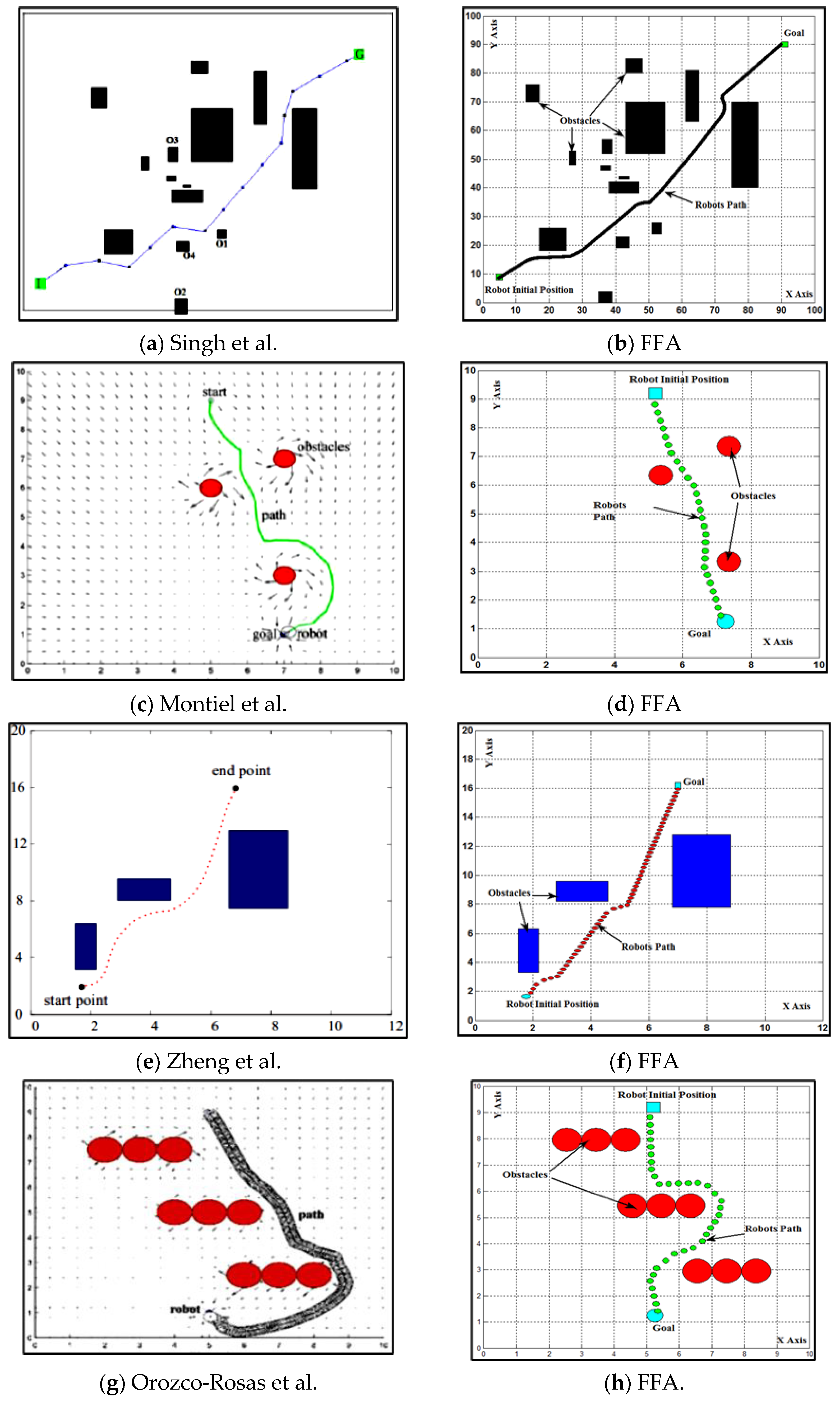
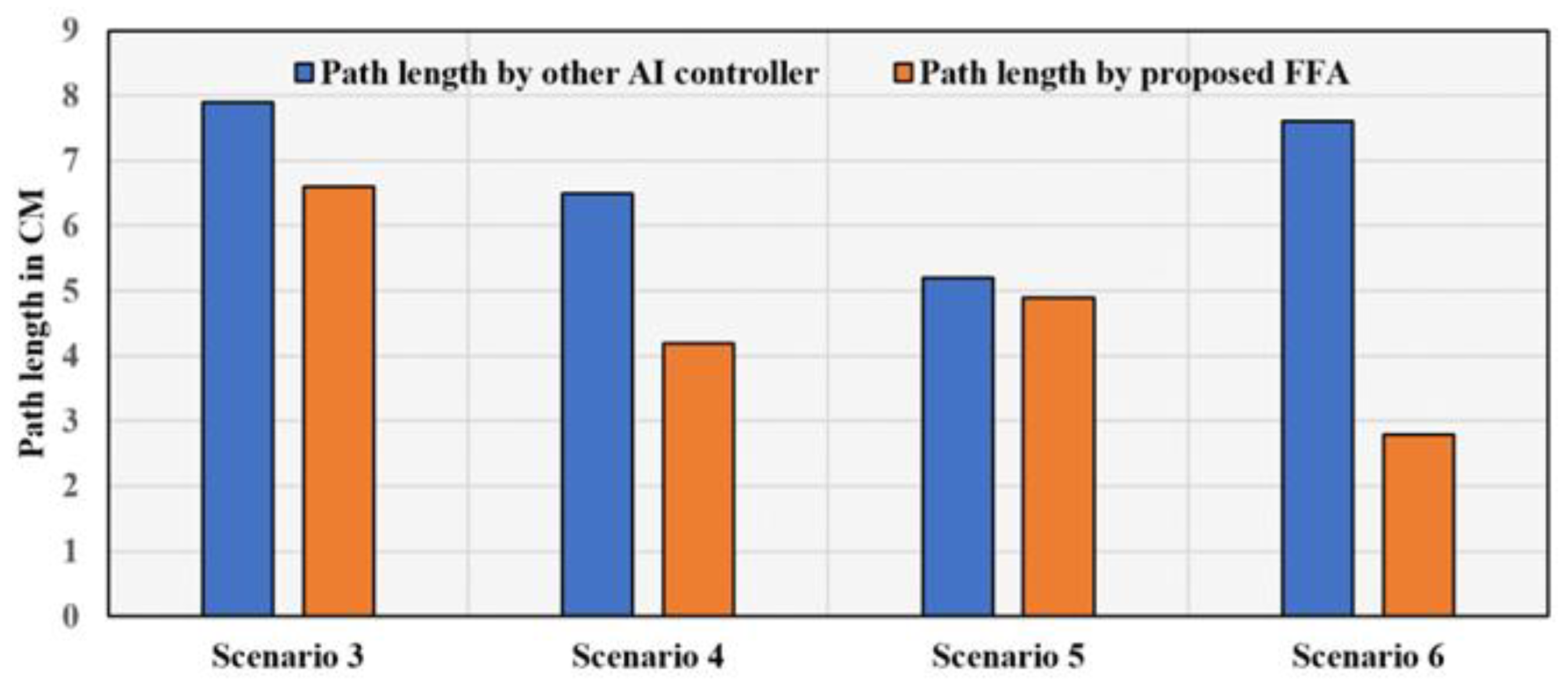
| S. N. | Start Point | Goal Point | Path Length (cm) by Other AI Controllers | Path Length (cm) by FFA Controller | % of Path Length Saved by FFA |
|---|---|---|---|---|---|
| Scenario-4 | (4,8) | (90,89) | 7.9 (Figure 21a) | 6.6 (Figure 21b) | 16.45 |
| Scenario-5 | (5,9) | (7,1) | 6.5 (Figure 21c) | 4.2 (Figure 21d) | 35.38 |
| Scenario-6 | (1.7,1.5) | (16.9,16) | 5.2 (Figure 21e) | 4.9 (Figure 21f) | 5.7 |
| Scenario-7 | (5,9) | (5,1) | 7.6 (Figure 21g) | 5.7 (Figure 21h) | 25 |
Disclaimer/Publisher’s Note: The statements, opinions and data contained in all publications are solely those of the individual author(s) and contributor(s) and not of MDPI and/or the editor(s). MDPI and/or the editor(s) disclaim responsibility for any injury to people or property resulting from any ideas, methods, instructions or products referred to in the content. |
© 2023 by the authors. Licensee MDPI, Basel, Switzerland. This article is an open access article distributed under the terms and conditions of the Creative Commons Attribution (CC BY) license (https://creativecommons.org/licenses/by/4.0/).
Share and Cite
Patle, B.K.; Patel, B.; Jha, A.; Kashyap, S.K. Self-Directed Mobile Robot Navigation Based on Functional Firefly Algorithm (FFA). Eng 2023, 4, 2656-2681. https://doi.org/10.3390/eng4040152
Patle BK, Patel B, Jha A, Kashyap SK. Self-Directed Mobile Robot Navigation Based on Functional Firefly Algorithm (FFA). Eng. 2023; 4(4):2656-2681. https://doi.org/10.3390/eng4040152
Chicago/Turabian StylePatle, Bhumeshwar K., Brijesh Patel, Alok Jha, and Sunil Kumar Kashyap. 2023. "Self-Directed Mobile Robot Navigation Based on Functional Firefly Algorithm (FFA)" Eng 4, no. 4: 2656-2681. https://doi.org/10.3390/eng4040152