Modelling Air Flow through Pneumatic Valves: A Brief Review with an Experimental Case Study

Abstract

Compressible flow models are commonly used for describing air flow through pneumatic valves. Because of the difficulties in predicting viscous losses, these models ultimately rely on experimental determination of coefficients. Different equations have been proposed for different fluid speeds, having the sonic fluid velocity as a reference mark. However, one might question whether a much simpler approach, where the fluid is considered as incompressible, would still give good results within the typical range of industrial applications. Moreover, practically all models presuppose that the valve output pressure decreases in time, as in a discharge process. This paper reviews some representative one-dimensional compressible flow models and discusses the appropriateness of using equations based solely on discharging flows. Two experimental circuits, where an air reservoir is pressurized and, subsequently, decompressed, are used for comparison between different flow models. It is shown that a simpler set of equations still produces acceptable results for practical pneumatic applications.

1. Introduction

Pneumatic valves are inherently complex in their internal geometry. The simplest spool-valve is three-dimensional by nature, which demands the complete solution of the Navier–Stokes plus the energy–balance equations to determine the pressure field within. Even in the simplest case scenario, where compressibility effects are small, still the Navier–Stokes equations, consisting of four non-linear partial, second order differential equations, are the basis for modelling the air flow through the valve. Since, to this day, no analytical solution exists for those complex equations, one needs to rely on numerical methods for modelling every other valve.

A simple approach to the problem (of modelling pneumatic valves) is to assume the flow as unidimensional, or, likewise, treat the variables involved in an averaged way. Therefore, we can simply refer to the input and output pressures with no concern about the pressure field within the valve itself. Such an approach is classical in engineering and was made possible through the Reynolds Transport Theorem. Yet, difficulties are not reduced and the price to be paid is the introduction of model constants to be experimentally determined. One model in particular has been generally adopted, even by in the ISO 6358 Standards [1], as will be described in this paper. Yet, its accuracy has been questioned [2], besides the fact that it requires the experimental determination of two constants. Our aim in this paper is to discuss the accuracy of the ISO 6358 model compared with other proposed equations.

2. Orifice Flow Theory

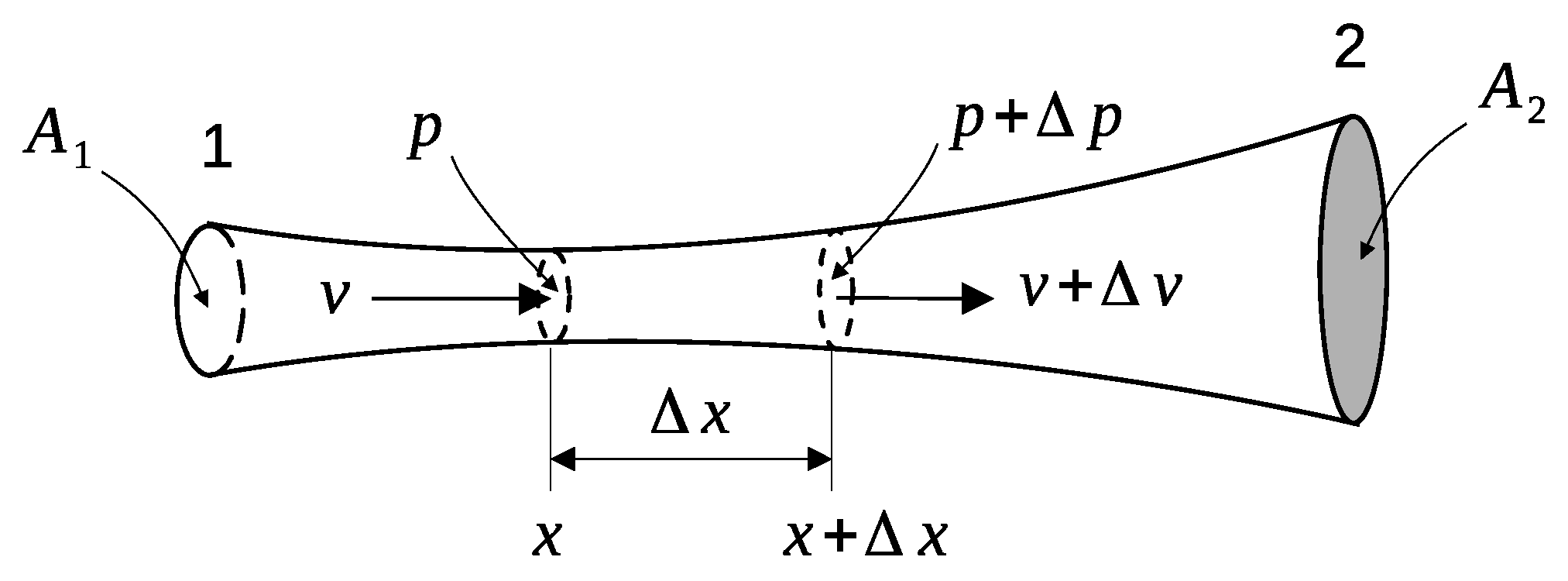
Air flows through valves and orifices are traditionally modeled after an initial application of the mass, momentum and energy balances over a small region in space, as illustrated in Figure 1, where a convergent–divergent nozzle is represented. As air flows from point 1 to point 2, there may or may not be a significant change in density. If the density does not change much, we may treat the flow as incompressible. However, this is not the general practice adopted in pneumatic valve design.

In what follows, we analyze the basis of compressible and incompressible flow modelling for the unidimensional flow represented in Figure 1 and further apply the resulting equations to the typical situation where flow is discharged and charged from and into an air tank. We begin with the incompressible flow approach.

It can be shown [3] that as long as the fluid speed remains below 0.3M (M is the Mach number), incompressible flow models can be applied and, in particular, the so-called “orifice equation” can be used; that is [4]

$$Q=\left\{\sqrt{\frac{2A_2^2}{\rho \left[1-{\left(\frac{A_2}{A_1}\right)}^2\right]}}\right\}\sqrt{p_1-p_2}=K\sqrt{p_1-p_2}$$

(1)

where Q is the volumetric flow; $p_1$ and $p_2$ are the pressures at points 1 and 2; $A_1$ and $A_2$ are the cross-sectional areas at points 1 and 2 (see Figure 1) and $\rho$ is the density of the fluid. Note that K is constant in Equation (1).

The mass flow, $\dot{m}$, can be obtained from (1) through the equation $\dot{m}=\rho Q$. Since we are considering that $\rho$ remains constant in space and in time, Equation (1) can be simplified to

$$\dot{m}=C\sqrt{p_1-p_2}$$

(2)

where $C=\rho K$. Here, the coefficient $C$ can be experimentally adjusted to include pressure losses.

If fluid compressibility is considered, Equation (2) cannot be used. Still, an analytical expression can be developed if we assume that the flow is inviscid, the process is adiabatic and the flow regime has reached the steady-state. Considering Figure 1 again, it can be shown that a momentum and a mass balance between points $x$ and $x+∆x$ produces the following equation [3]

$$\frac{dp}{\rho }+d\left(\frac{v^2}{2}\right)=0$$

(3)

where $\rho$, $p$ and $v$ are the density, pressure and velocity, respectively. As $∆x$, in Figure 1, becomes infinitesimal ($∆x\to dx$, $∆v\to dv$ and $∆p\to dp$).

The assumption of an adiabatic flow, for which $p/{\rho }^{\gamma }=C_{\gamma }$ ($C_{\gamma }$ is a constant and $\gamma$ is the ratio of specific heat capacities) allows us to integrate Equation (3) between points 1 and 2, resulting in

$$\frac{1}{2}\left(v_2^2-v_1^2\right)=C_{\gamma }^{\left(\frac{1}{\gamma }\right)}\left(\frac{\gamma }{\gamma -1}\right)\left[{p_1}^{\left(\frac{\gamma -1}{\gamma }\right)}-{p_2}^{\left(\frac{\gamma -1}{\gamma }\right)}\right]$$

(4)

Equation (4) can be written in a more meaningful form if we write $C_{\gamma }^{1/\gamma }=p_1^{1/\gamma }/{\rho }_1$. After some mathematical work, the following equation is obtained

$$v_2^2-v_1^2=2R{T}_1\left(\frac{\gamma }{\gamma -1}\right)\left[1-{\left(\frac{p_2}{p_1}\right)}^{\left(\frac{\gamma -1}{\gamma }\right)}\right]$$

(5)

Where R = 287 J/kgK is the gas constant for air and $T_1$ is the absolute temperature (K) inside the tank.

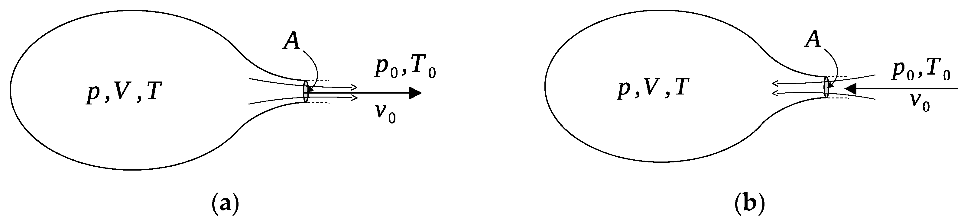
Of particular interest are the situations where air contained in a tank (a) discharges into the atmosphere through an orifice (or a valve), as illustrated in Figure 2a,b, is pressurized by an incoming flow, as shown in Figure 2b. Considering that air flows from point 1 to point 2, in Equation (4), we have that

• $v_1=0$, $v_2=v_0$, $p_1=p$ and $p_2=p_0$ for the tank discharge (Figure 2a);
• $v_1=v_0$, $v_2=0$, $p_1=p_0$ and $p_2=p$ for the tank pressurization (Figure 2b).

Substituting the values at points 1 and 2 for each case represented in Figure 2 into Equation (5), and considering the speed of sound at the tank nozzle, $c_0=\sqrt{\gamma R{T}_0}$, and the corresponding Mach number, $M_0=v_0/c_0$, it is possible to arrive at the following equations for the pressure ratio $r_p=p_0/p_1$

$$\left\{\begin{array}{ll}{r}_p={\left[1-\left(\frac{T_0}{T}\right)\left(\frac{\gamma -1}{2}\right)M_0^2\right]}^{\frac{\gamma }{\gamma -1}}& \mathrm{D}\mathrm{i}\mathrm{s}\mathrm{c}\mathrm{h}\mathrm{a}\mathrm{r}\mathrm{g}\mathrm{e} \\ r_p={\left[\left(\frac{\gamma -1}{2}\right)M_0^2+1\right]}^{-\left(\frac{\gamma }{\gamma -1}\right)}& \mathrm{C}\mathrm{h}\mathrm{a}\mathrm{r}\mathrm{g}\mathrm{e}\end{array}\right.$$

(6)

• Remarks

1.

The critical pressure ratio, b, is defined as the ratio, $r_p$, for which sonic speed is attained at the nozzle. Its value is not the same for charging and discharging, being dependent on the ratio between nozzle and tank temperatures, $T_0/T$, at discharge (but not on charge). Although this fact was recognized long ago [5], it has been ignored in most of the references on the topic (see, for example, references [6,7,8]), where in both charge and discharge, $b$ is obtained from the second equation in (6) by making $M_0=1$; that is

$$b={\left(\frac{\gamma +1}{2}\right)}^{-\left(\frac{\gamma }{\gamma -1}\right)}={\left(\frac{2}{\gamma +1}\right)}^{\frac{\gamma }{\gamma -1}}$$

(7)

2.

In spite of the fact that Equation (6) makes no reference to the nozzle geometry, the Mach number at the nozzle, $M_0$, is directly related to the cross-sectional area, A, and the way it changes along the $x$ axis (Figure 1). For instance, if pressure decreases along the flow direction, it can be shown that, for subsonic flows, the fluid velocity increases as A is reduced. An opposite effect exists when the flow becomes supersonic. At sonic speed, $A$ reaches a minimum value [9];

3.

Considering a hypothetical scenario where the pressure tank discharges into the absolute vacuum ($p_0=0$ and $r_p=0$), the first equation in (6) fails to represent the flow. To see that, we note that for a perfect gas, $p_0=0$ implies in $T_0=0$. As a result, the first equation in (6) would result in $0=1$, which is incongruent. The second equation in (6) also fails to represent the flow at $r_p=0$. In addition, liquefaction of the gaseous components of air would not allow for using the perfect-gas hypothesis at very low temperatures. These considerations pose a limitation on the use of Equation (6) for adiabatic flows through orifices.

The velocity and the mass flow at the nozzle, $v_0$ and ${\dot{m}}_0$, can be obtained from Equation (5) for both situations shown in Figure 2. Therefore, $v_0$ is given by

$$\left\{\begin{array}{ll}{v}_0=\sqrt{2RT}\sqrt{\left(\frac{\gamma }{\gamma -1}\right)\left[1-{\left(\frac{p_0}{p}\right)}^{\left(\frac{\gamma -1}{\gamma }\right)}\right]}& \mathrm{D}\mathrm{i}\mathrm{s}\mathrm{c}\mathrm{h}\mathrm{a}\mathrm{r}\mathrm{g}\mathrm{e} \\ v_0=\sqrt{2R{T}_0}\sqrt{\left(\frac{\gamma }{\gamma -1}\right)\left[{\left(\frac{p_0}{p}\right)}^{-\left(\frac{\gamma -1}{\gamma }\right)}-1\right]}& \mathrm{C}\mathrm{h}\mathrm{a}\mathrm{r}\mathrm{g}\mathrm{e}\end{array}\right.$$

(8)

To obtain the mass flow, we make $v_0=\dot{m}/\left({\rho }_{0}A\right)$

$$\left\{\begin{array}{ll}\dot{m}={\rho }_{0}A\sqrt{2RT}\sqrt{\left(\frac{\gamma }{\gamma -1}\right)\left[1-{\left(\frac{p_0}{p}\right)}^{\left(\frac{\gamma -1}{\gamma }\right)}\right]}& \mathrm{D}\mathrm{i}\mathrm{s}\mathrm{c}\mathrm{h}\mathrm{a}\mathrm{r}\mathrm{g}\mathrm{e} \\ \dot{m}={\rho }_{0}A\sqrt{2R{T}_0}\sqrt{\left(\frac{\gamma }{\gamma -1}\right)\left[{\left(\frac{p_0}{p}\right)}^{-\left(\frac{\gamma -1}{\gamma }\right)}-1\right]}& \mathrm{C}\mathrm{h}\mathrm{a}\mathrm{r}\mathrm{g}\mathrm{e}\end{array}\right.$$

(9)

The discharge equation for $\dot{m}$ has been extensively used in pneumatic circuits to simulate flow through valves and is usually represented in a different way, following the work of St. Venant and Wantzel in 1839 [6]. To modify the discharge equation, we first write $p/{\rho }^{\gamma }=p_0/{\rho }_0^{\gamma }$. Then, we obtain ${\rho }_0$ from this last expression and substitute it into the first equation in (9). Finally, we write $\rho =p/\left(RT\right)$ and, after some algebraic work, arrive at the following expression for $\dot{m}$

$$\dot{m}=pA\mathsf{\Psi }\sqrt{\frac{2}{RT}}$$

(10)

where $\mathsf{\Psi }$, known as the “flow function”, is given by

$$\mathsf{\Psi }=\sqrt{\left(\frac{\gamma }{\gamma -1}\right)\left[{\left(\frac{p_0}{p}\right)}^{\frac{2}{\gamma }}-{\left(\frac{p_0}{p}\right)}^{\frac{\gamma +1}{\gamma }}\right]}$$

(11)

The following expression is obtained for $d\mathsf{\Psi }/d{r}_p=0$ (remember that $r_p=p_0/p$)

$$\left(\frac{2}{\gamma }\right){r_p}^{\left(\frac{2-\gamma }{\gamma }\right)}-\left(\frac{\gamma +1}{\gamma }\right){r_p}^{\left(\frac{1}{\gamma }\right)}=0$$

(12)

Equation (12) can be solved for $r_p$, which yields the maximum value of the flow function, $\mathsf{\Psi }$, in Equation (11). The solution of Equation (12) is

$$r_p=b={\left(\frac{2}{\gamma +1}\right)}^{\frac{\gamma }{\gamma -1}}$$

(13)

which is the critical pressure ratio, already obtained in Equation (7) for the case where the air tank is being charged. Substituting $b$, given by Equation (13), into the first equation in (8), we obtain the maximum value of the air velocity when the tank is being discharged, $v_0=v_{max}$, as

$$v_{max}=c\sqrt{\frac{2}{\gamma +1}}$$

(14)

where $c=\sqrt{\gamma RT}$ is the speed of sound at temperature T. Note that $v_{max}$ is close to sonic speed (for $\gamma =1.4$, $v_{max}=0.913c$).

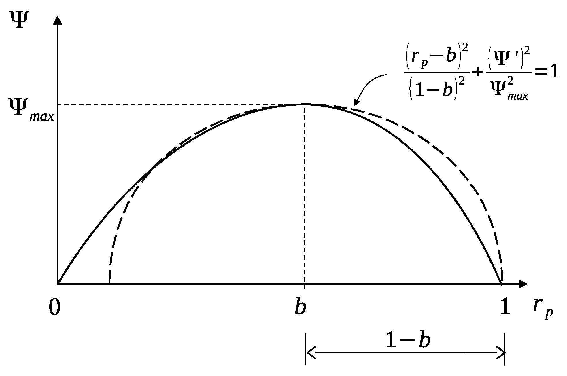
The ratio $b=p_0/p$ corresponding to the maximum value of $\mathsf{\Psi }$ has been used as a divider in compressible flow discharge. Flows where $0<r_p<b$ are termed as critical flows while flows where $b<r_p<1$ are denominated subcritical flows [10]. Figure 3 illustrates this division in a graphical manner. Observe that the function $\mathsf{\Psi }\left(r_p\right)$ resembles half of an ellipse at the interval $b<r_p<1$. Figure 3 shows the ellipse as a dashed curve and its corresponding equation.

We may write the ellipse equation in Figure 3 as ${\mathsf{\Psi }}^{\prime }\left(r_p\right)$, as follows

$${\mathsf{\Psi }}^{\prime }={\mathsf{\Psi }}_{max}\sqrt{1-{\left(\frac{r_p-b}{1-b}\right)}^2}$$

(15)

where ${\mathsf{\Psi }}_{max}$ is obtained by substituting r_p, given by Equation (13) into Equation (11), resulting in the following expression

$${\mathsf{\Psi }}_{max}={\left(\frac{2}{\gamma +1}\right)}^{\frac{1}{\gamma -1}}\sqrt{\frac{\gamma }{\gamma +1}}$$

(16)

The theory presented so far led us to two equations that describe the steady-state behavior of incompressible and compressible air flows as they discharge through a nozzle; that is, Equations (2) and (10), plus the elliptical flow function approximation (15). Although pressure losses due to viscosity effects and the influence of nozzle geometry can be factored into the coefficient $C$, in Equation (2), the compressible flow model, given by Equation (10), assumes that the flow is inviscid and makes no particular reference to the nozzle geometry. One simple adjustment aiming to correct the mass flow to include these effects consists in adding a discharge coefficient, $C_d$, to Equation (10), as follows

$$\dot{m}=C_{d}pA\mathsf{\Psi }\sqrt{\frac{2}{RT}}$$

(17)

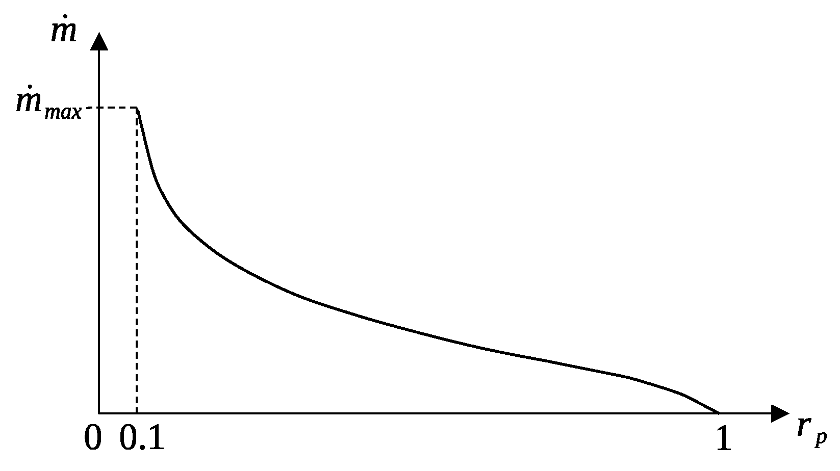
Like the fluid velocity, $v_0$, the mass flow, $\dot{m}$, has a maximum at $r_p=b$ in the case where the upstream pressure, p, is kept constant. This is very important, because in the situation depicted in Figure 2a, where no flow enters the air tank, such assumption is not correct. The fact that $\dot{m}$ achieves a maximum when $p$ is constant can be concluded by a simple observation of Equation (17), where all the terms on the right-hand side, except the flow function $\mathsf{\Psi }$, become constant, so that $\dot{m}$ has the same behaviour as $\mathsf{\Psi }$ (see Figure 3). When the upstream pressure, p, is not constant, as is the case in Figure 2a, we can write $p=p_0/r_p$ in Equation (17) so that the mass flow can then be written as $\dot{m}\left(r_p\right)$, as follows

$$\dot{m}=K_T\left(\frac{\mathsf{\Psi }}{r_p}\right)$$

(18)

where $K_T$ is given by

$$K_T=C_d{p}_{0}A\sqrt{\frac{2}{RT}}$$

(19)

Assuming that $K_T$ is constant, the mass flow, $\dot{m}$, can be plotted against the pressure ratio, $r_p$, for a vessel discharging into the atmosphere, as in Figure 2a. Here, we have assumed the typical industrial range for the pressure ratio, 0.1$\le r_p\le 1$. Figure 4 shows the curve $\dot{m}\left(r_p\right)$.

The problem in using Equation (17) in the whole range of the pressure ratio was addressed by Lord Rayleigh in 1916 [4], who experimentally proved the non-validity of Equation (18) for the interval $0\le r_p\le 0.25$, where the mass flow would, in fact, be constant for a constant value of $p$. His results contradicted a previous statement made by Osborne Reynolds, in 1885. According to Hartshorn [11], Reynolds wrote that the mass flow would remain constant within the interval $0\le r_p\le 0.53$. Hartshorn concluded that neither Rayleigh nor Reynolds were 100% correct, for experiments showed that the interval limit where the mass flow is constant depends on the type of nozzle that is used. According to his experiments, the mass flow would become constant whenever $0\le r_p\le L$, with L varying from 0.2 to 0.8, depending on the shape of the discharge nozzle. Figure 5 has been based on the experimental curves published by Hartshorn and illustrates the experimental results that he obtained.

In summary, the following equations can be used for adiabatic discharges through orifices and valves only for the case where $p$ is constant

$$\left\{\begin{array}{lll}\dot{m}=C_{d}pA\mathsf{\Psi }\sqrt{\frac{2}{RT}}& \mathrm{w}\mathrm{h}\mathrm{e}\mathrm{n} & L<r_p\le 1\\ \dot{m}={\dot{m}}_{max}& \mathrm{w}\mathrm{h}\mathrm{e}\mathrm{n}& 0\le r_p\le L\end{array}\right.$$

(20)

Attempts to find the experimental curves for $\dot{m}$ have followed ever since. For instance, in 1955, Druett obtained experimental curves for divergent conic-shaped orifices [12]. However, a somewhat common practice is to assume $L=0.528$, corresponding to the critical pressure ratio, $b$, for $\gamma =1.4$ (see, for example, [2,13,14,15,16,17,18,19,20,21]).

3. The ISO 6358 Equations

As is usually the case, the need to find a relation between mass flow and pressure has led to attempts to standardize the mathematical model for orifice and valve flows in pneumatic circuits. One known standard that has been extensively used is the ISO 6358, where the following equations are recommended for modelling pneumatic valve flows [6]

$$\left\{\begin{array}{lll}\dot{m}=\left(C{\rho }_{r}p\sqrt{\frac{T_r}{T}}\right)\sqrt{1-{\left(\frac{r_p-L}{1-L}\right)}^2}& \mathrm{w}\mathrm{h}\mathrm{e}\mathrm{n} & L<r_p\le 1\\ \dot{m}=C{\rho }_{r}p\sqrt{\frac{T_r}{T}}& \mathrm{w}\mathrm{h}\mathrm{e}\mathrm{n}& 0\le r_p\le L\end{array}\right.$$

(21)

where ${\rho }_r$ and $T_r$ are the density and absolute temperature measured at a pre-established rated condition, defined by ISO as $T_r=293.15 \mathrm{K}$, $p_r=100 \mathrm{k}\mathrm{P}\mathrm{a}$, ${\rho }_r=1.185 \mathrm{k}\mathrm{g}/{\mathrm{m}}^3$ for a relative humidity of 65% and a corresponding gas constant $R=288 \mathrm{J}/\mathrm{k}\mathrm{g}·\mathrm{K}$. The coefficient $C \left({\mathrm{m}}^3/\mathrm{P}\mathrm{a}·\mathrm{s}\right)$ is denominated “sonic conductance” and, together with the “sonic pressure ratio”, $L$, must be experimentally obtained.

The ISO standard uses the elliptical approximation, ${\mathsf{\Psi }}^{\prime }$, given by Equation (15), as can be seen in second radicand of the first equation in (21). In fact, the first equation in (21) can be obtained by first substituting $\mathsf{\Psi }$ with ${\mathsf{\Psi }}^{\prime }$, in Equation (17), as follows

$$\dot{m}=p{C}_d\sqrt{\frac{1}{RT}}\sqrt{1-{\left(\frac{r_p-L}{1-L}\right)}^2}$$

(22)

We can then use the perfect gas equation at a given reference state, $p_r={\rho }_{r}R{T}_r$, to eliminate the constant $R$ from Equation (22)

$$\dot{m}=\left(C{\rho }_{r}p\sqrt{\frac{T_r}{T}}\right)\sqrt{1-{\left(\frac{r_p-L}{1-L}\right)}^2}$$

(23)

where

$$C=A{C}_d{\mathsf{\Psi }}_{max}\sqrt{\frac{2}{p_r{\rho }_r}}$$

(24)

Equation (21) has been widely used to this date for modelling pneumatic valve flows. The usual procedure, however, is to skip the experimental determination of the sonic pressure ratio, L, and use L = 0.528, which, as we have seen in the previous section, is not a safe assumption (Figure 5). On the other hand, the ISO 6358 Standard is highly demanding, requiring the experimental determination of two coefficients (L and C). The difficulties involved in determining the exact nature of the gas compression/expansion, being generally polytropic can move $\gamma$ away from the adiabatic index ($\gamma =1.4$), thus changing the value of $b$ in Equation (13). For an assumed range $1<\gamma <1.7$, we would have $0.48<b<0.605$ [22]. In addition, as mentioned in the previous section, values of L as low as 0.2 were experimentally obtained. In fact, due to the difficulty in obtaining L, it is tempting to attribute a random value to L, perhaps based on some intuitive criteria, as can be concluded by reading some of the several works published on pneumatic circuits.

One question to be asked here is whether a simpler model such as the one given by Equation (2) could be used for modelling mass flows through valves. Bobrow and McDonell [2], for example, stated that “…nearly all previous results on pneumatic control incorrectly assume (14) is true”, where (14) is a reference to the ISO equations in their paper. They obtained better results with the following equations, used in the context of a proportional valve connected to a cylinder

$$\left\{\begin{array}{ll}\dot{m}=k_1\sqrt{p-p_0}& \mathrm{C}\mathrm{h}\mathrm{a}\mathrm{r}\mathrm{g}\mathrm{i}\mathrm{n}\mathrm{g}\\ \dot{m}=k_2\left(p-p_0\right)& \mathrm{D}\mathrm{i}\mathrm{s}\mathrm{c}\mathrm{h}\mathrm{a}\mathrm{r}\mathrm{g}\mathrm{i}\mathrm{n}\mathrm{g}\end{array}\right.$$

(25)

where the coefficients $k_1$ and $k_2$ depend on the electric current that is applied to the proportional valve, according to the original paper [2].

We would like to investigate whether Equation (25) can still be used to model air flow through valves and orifices when $k_1$ and $k_2$ are constants. In fact, the first equation in (25) is, precisely, the incompressible flow model (2), with $C=k_1$. The linear relation indicated by the second equation, on the other hand, characterizes a laminar flow [4]. If these equations are able to represent flows through actual valves, the difficulties involved in determining L in Equation (21) are bypassed. We deal with this matter in the following section.

4. Numerical Modelling and Simulation

Consider the pressurization and subsequent decompression of an air tank, as shown in Figure 6. The schematics shown in the figure include elements that will be referred to, when we describe the test rig used in the experimental procedure.

To pressurize the tank 1, in Figure 6a, the unidirectional flow–control valve 2 can be adjusted between totally closed and totally open. The manually activated directional valve 3 provides a constant pressure, p, at the input of valve 2 while the tank pressure, $p_0$, changes from 0 to 0.6 MPa (gauge). The pressure evolution in time can be visually seen with the help of gauge 5 and measured in a timely manner by transducer 4, which sends data to an analog–digital converter connected to a computer. Depressurization (Figure 6b) is performed by inverting the position of valve 2 and closing it with the air tank pressure at 0.6 MPa, while air escapes to the atmosphere through valve 6. Note that p, at the valve 6 input, is variable this time, while $p_0$ remains constant.

Mass conservation can be applied to both situations in Figure 6. Considering that the air tank volume is V and that it remains at a constant temperature, T, the following equation is obtained

$$\dot{m}+\left(\frac{V}{RT}\right)\frac{dp}{dt}=0$$

(26)

where $\dot{m}$ is negative when flowing into the air tank, as in Figure 6a, and positive otherwise (Figure 6b). If we write $C_0=\left(RT\right)/V$, Equation (26) can be written in a more convenient form as

$$\frac{dp}{dt}=-C_0\dot{m}$$

(27)

To circumvent the complexities of the analytical solutions for (27), when different expressions for $\dot{m}\left(p\right)$ are used, we have solved this equation numerically.

Table 1. Summary of the different expressions for the air mass flow.

Equation Label	Equation
Equation (2)	$\dot{m}=C_1\sqrt{p-p_0}$
Equation (21)	$\left\{\begin{array}{lll}\dot{m}=C_{2}p\sqrt{1-{\left(\frac{r_p-L}{1-L}\right)}^2}& \mathrm{w}\mathrm{h}\mathrm{e}\mathrm{n} & L<r_p\le 1\\ \dot{m}=C_{2}p& \mathrm{w}\mathrm{h}\mathrm{e}\mathrm{n}& 0\le r_p\le L\end{array}\right.$
Equation (25)	$\dot{m}=C_3\left(p-p_0\right)$

summarizes the equations for $\dot{m}\left(p\right)$ we have seen so far, for the situation where the air tank discharges into the atmosphere. In the table, we have grouped different factors as constants $C_1$ through $C_3$. Since the great majority of scientific and engineering works make use of only one model regardless of the direction of the air flow, only the equations corresponding to the tank discharge are being considered in Table 1. Incidentally, both Equation (25) are represented, given that the first equation in (25) corresponds exactly to the incompressible flow model (2).

Each equation in Table 1 demands the knowledge of a constant, which must be determined through experimental data fitting. An easy way to make any of these models describe the actual air flow, however, is to change these constants into coefficients. For instance, considering a general coefficient $C_k$, we might think of a polynomial expansion of degree $N$, $C_k=\sum _n{a}_n{r}_p^n$ ($n=0\dots N$), as proposed in [13] for the ISO Equation (21). We do not favor this approach, given that, virtually, any model in Table 1 can be adjusted to fit experimental results by correctly choosing the new constants of the coefficient $C_k$. Moreover, once the polynomial equation for $C_k$ is introduced back into its corresponding mathematical model, we end up with a totally strange equation, for which no physical background can be traced.

In Table 1, the constants $C_1$, $C_2$ and $C_3$ are given by:

$$\left\{\begin{array}{l}{C}_1=\sqrt{\frac{2A_2^2}{\rho \left[1-{\left(\frac{A_2}{A_1}\right)}^2\right]}}\\ C_2=C{\rho }_{r}p\sqrt{\frac{T_r}{T}}\\ C_3=k_2\end{array}\right.$$

(28)

The combination of the equations in Table 1 and the differential Equation (27) results in three mathematical models for the pressure inside the air tank in Figure 6, as listed in

Table 2. Mathematical models for the pressure inside the air tank.

Model	Equation
Model 1	$\frac{dp}{dt}=-C_0{C}_1\sqrt{p-p_0}$
Model 2	$\left\{\begin{array}{lll}\frac{dp}{dt}=-C_0{C}_{2}p\sqrt{1-{\left(\frac{r_p-L}{1-L}\right)}^2}& \mathrm{w}\mathrm{h}\mathrm{e}\mathrm{n} & L<r_p\le 1\\ \frac{dp}{dt}=-C_0{C}_{2}p& \mathrm{w}\mathrm{h}\mathrm{e}\mathrm{n}& 0\le r_p\le L\end{array}\right.$
Model 3	$\frac{dp}{dt}=-C_0{C}_3\left(p-p_0\right)$

.

We have solved each equation in Table 2 for $p\left(t\right)$, adjusting constants $C_1$ through $C_3$ so that $p\left(0\right)=0 \mathrm{M}\mathrm{P}\mathrm{a}$ and $p\left(12\right)=0.7 \mathrm{M}\mathrm{P}\mathrm{a}$, simulating the pressurization of the air tank in Figure 6a. In a reverse order, we also simulated the decompression of the air tank for $p\left(0\right)=0.7 \mathrm{M}\mathrm{P}\mathrm{a}$ and $p\left(30\right)=0 \mathrm{M}\mathrm{P}\mathrm{a}$. The time setting for the simulation has been based on experimental data to be introduced in the following section. Considering an air tank volume $V=0.4 \mathrm{L}$ and assuming that the air temperature is kept at $T=293 \mathrm{K}$, the constant $C_0$ can be calculated as

$$C_0=\frac{RT}{V}=\frac{287\frac{\mathrm{J}}{\mathrm{k}\mathrm{g}·\mathrm{K}}\times 293 \mathrm{K}}{\left(0.4\times {10}^{-3}\right){\mathrm{m}}^3}=\left(2.1\times {10}^8\right)\frac{\mathrm{J}}{\mathrm{k}\mathrm{g}·{\mathrm{m}}^3}$$

(29)

We have assumed $L=0.528$ and $p_0=0.1 \mathrm{M}\mathrm{P}\mathrm{a}$. Simulation results, obtained by using the 4th order Runge–Kutta method to solve the equations in Table 2, are shown in Figure 7. Figure 7a,b show the evolution in time of the pressure inside the air tank. In both cases, there is a closer match between results given by models 1 and 2. This is due to the much higher mass flow at the beginning when the linear model 3 is used, as can be seen in Figure 7c,d. Note the constant mass flow during $0\le t\le 0.528$ at pressurization when model 2 is used. This is justified by the fact that model 2 is based on the theoretical–experimental approach explained in the previous section where the mass flow becomes constant when the pressure ratio drops below a given value of $r_p$ (see Figure 5).

It is very important to observe the values of the constants $C_1$, $C_2$ and $C_3$ change significantly between decompression and pressurization. As a matter of fact, they also change with the flow–control valve adjustment, as will be seen in the following section, where we present experimental results that will help us better compare the models in Table 2.

5. Comparison with Experimental Results

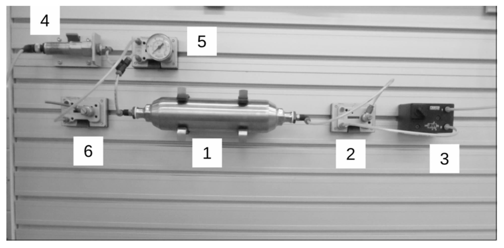
Figure 8 shows the pneumatic test rig used to obtain the curve $p\left(t\right)$ for the two situations displayed in Figure 6. The technical specifications for each component are given in

Table 3. Technical specifications for the test rig components.

Component Number	Commercial Model
1	Air reservoir FESTO. Model CRVZS-0,4 160234 (0.4 liters)
2	Flow–control valve FESTO. Model 152881
3	Festo 3/2 valve with selector switch. Model 152863
4	Pressure transmitter FESTO. Model SDET-22T-D10-G14-U-M12 (1% accuracy)
5	Pressure gauge FESTO. Model 152865
6	FESTO 152881

. All components are interconnected through plastic tubing whose external/internal diameters are 4 mm and 2.5 mm, respectively.

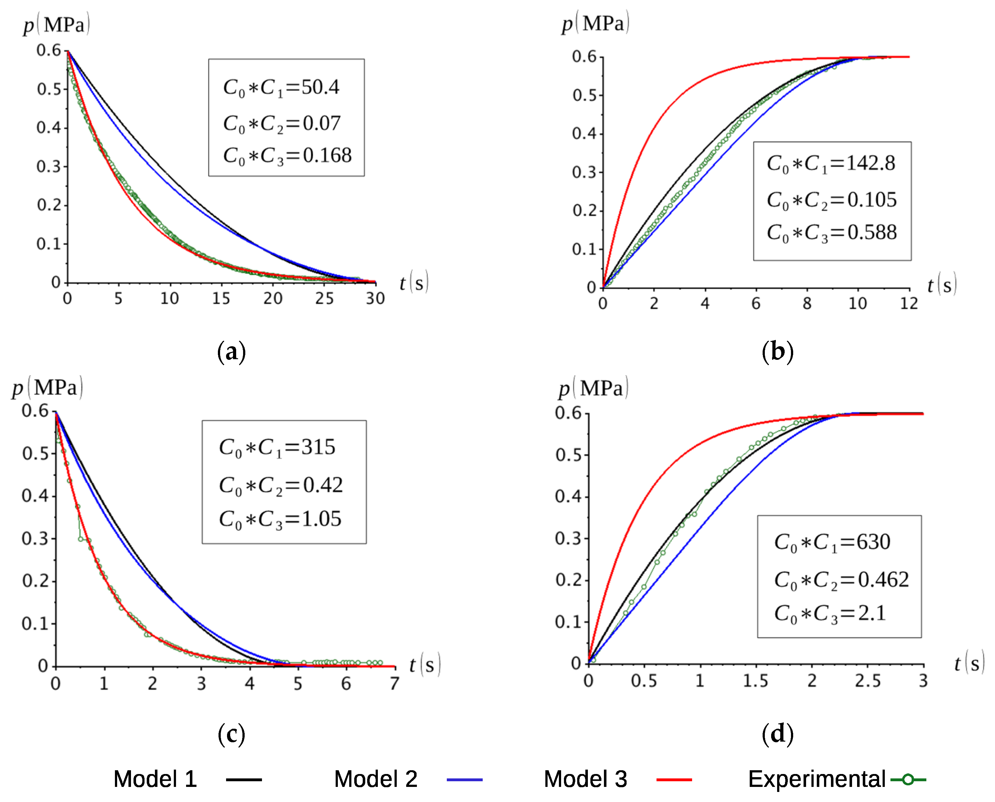
A comparison between experimental results and the theoretical curves is shown in Figure 9 for two opening states of the flow–control valves. First, the valve was approximately 5% open. The curves corresponding to the decompression and pressurization of the air tank for this first setting are shown in Figure 9a,b, respectively. The second set of experimental data was obtained for a 100% opening of the flow control valves, for which corresponding curves are shown in Figure 9c,d, for decompression and pressurization, respectively. The curves were fitted so that they would match experimental data at $p=0.6 \mathrm{M}\mathrm{P}\mathrm{a}$ and $p=0 \mathrm{M}\mathrm{P}\mathrm{a}$ (gauge).

At a first glance, we conclude that the third model produces a far better approximation to experimental data when the air tank is discharging into the atmosphere (Figure 9a,c). On the other hand, both the incompressible flow model 1 and the ISO model 2 are better when the tank is being charged (Figure 9b,d). It is, therefore, reasonable, to prefer the one-constant modelling Equation (25) instead of the two-constant ISO Equation (21).

The reason why the linear dependence between flow and pressure provides a better approximation during discharge is a challenging one. As we already mentioned, the assumption of a laminar flow on discharge would help to explain this fact. We believe that a more detailed analysis would require the numerical solution of the Navier–Stokes equations. This is certainly one possibility for further developments to be pursued in a future work.

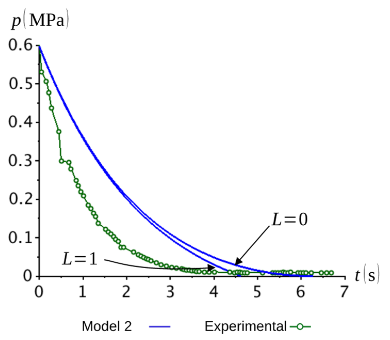
One might wonder whether the choice for $L$ in model 2 would be the reason why the ISO model does not provide the best fit during tank discharge. To verify this, we simulated the same case shown in Figure 9c using the two extreme values of $L$, 0 and 1. The results are presented in Figure 10. Even with these changes we could not obtain a better fitting, which suggests that Equation (21) is not the best option for the case where the tank is depressurized. Moreover, the simpler incompressible model 1 also provides a good approximation for the case where the tank is being charged, with only one constant to be adjusted. We thus come to the same conclusion found in reference [2] and agree that Equation (25) best fits our experimental data.

6. Conclusions

In this paper, we reviewed the most common models for pneumatic valve flow, beginning at the very foundations of the currently accepted models. We showed that equations are not the same for discharging and charging vessels and discussed the application of classical compressible-flow equations in real-life pneumatic applications, where we could see that the simple assumption of fluid incompressibility can be safely applied for the usual pressure range in industrial applications when the flow direction is towards pressurization of the receiving pneumatic element, which, in our case, was an air tank. The similarity between the results obtained using compressible and incompressible models, in this case, explains why we do not find any publication, except from the one in reference [2], where incompressible flow equations are applied. Incidentally, a numerical flow analysis carried out for a spool valve has recently shown that the internal valve flow is predominantly incompressible [23]. This fact may certainly be considered in a future analysis of the problem.

Last, it is interesting that an even simpler relation provided a more accurate match with experimental values when the flow direction was directed towards depressurizing the air tank. An actual explanation for this behavior is not in the scope of this paper and can also be an inspiring topic for future work. In the end, we have concluded that it is safe to use a simple model where only one constant needs to be experimentally determined, instead of the more complex ISO 6358 model, where two different constants are required.

References

- ISO 6358-1: 2013; Pneumatic Fluid Power–Determination of Flow Rate Characteristics of Components Compressible Fluids–Part 1: General Rules and Test Methods for Steady-State Flow. ISO: Geneva, Switzerland, 2013. Available online: https://www.iso.org/standard/56612.html (accessed on 13 October 2023).
- Bobrow, J.E.; McDonell, W. Modeling, identification, and control of a pneumatically actuated, force controllable robot. IEEE Trans. Robot. Autom. 1998, 14, 732–742. [Google Scholar] [CrossRef]
- Pritchard, P.J.; Mitchell, J.W. Fox and McDonald’s Introduction to Fluid Mechanics, 8th ed.; John Wiley & Sons: New York, NY, USA, 2011; pp. 675–680. [Google Scholar]
- Costa, G.K.; Sepehri, N. Hydrostatic Transmissions and Actuators: Operation, Modelling and Applications; John Wiley & Sons: Chichester, UK, 2015; pp. 81, 86. [Google Scholar]
- Lord Rayleigh, O.M.F.R.S. On the discharge of gases under high pressures. Lond. Edinb. Dublin Philos. Mag. J. Sci. 1916, 32, 177–187. [Google Scholar] [CrossRef]
- Beater, P. Pneumatic Drives: System Design, Modelling and Control; Springer: Berlin, Germany, 2007; pp. 29–31. [Google Scholar]
- Sanville, F.E. A New Method of Specifying the Flow Capacity of Pneumatic Fluid POWER Valves. In Proceedings of the Second Fluid Power Symposium, Guildford, UK, 4–7 January 1971. [Google Scholar]
- Pasieka, L. The applicability of the mass-flow-model according to ISO 6358 with the parameter critical conductance c and critical pressure ratio b for gases in high-pressure range up to 300 bar. In Proceedings of the 12th International Fluid Power Conference (12. IFK), Dresden, Germany, 12–14 October 2020. [Google Scholar]
- Zucker, R.D.; Biblarz, O. Fundamentals of Gas Dynamics, 2nd ed.; John Wiley & Sons. Inc.: Hoboken, NJ, USA, 2002; pp. 119–120. [Google Scholar]
- Perry, J.A., Jr. Critical Flow Through Sharp-Edged Orifices. Trans. Am. Soc. Mech. Eng. 1949, 71, 757–763. [Google Scholar] [CrossRef]
- Hartshorn, L. The Discharge of Gases under High Pressures. Phil. Mag. 1916, 32, 178–188. [Google Scholar]
- Druett, H.A. The Construction of Critical Orifices Working with Small Pressure Differences and Their Use in Controlling Airflow. Br. J. Ind. Med. 1955, 12, 65–70. [Google Scholar] [CrossRef] [PubMed]
- Pugi, L.; Malvezzi, M.; Allotta, B.; Banchi, L.; Presciani, P. A parametric library for the simulation of a Union Internationale des Chemins de Fer (UIC) pneumatic braking system. Proc. Inst. Mech. Eng. Part F J. Rail Rapid Transit 2004, 218, 117–132. [Google Scholar] [CrossRef]
- Rahman, R.A.; He, L.; Sepehri, N. Design and experimental study of a dynamical adaptive backstepping–sliding mode control scheme for position tracking and regulating of a low-cost pneumatic cylinder. Int. J. Robust Nonlinear Control. 2016, 26, 853–875. [Google Scholar] [CrossRef]
- Pawananont, K.; Leephakpreeda, T. Sequential Control of Multichannel On–Off Valves for Linear Flow Characteristics Via Averaging Pulse Width Modulation without Flow Meter: An Application for Pneumatic Valves. J. Dyn. Syst. Meas. Control. 2019, 141, 011007. [Google Scholar] [CrossRef]
- Mandali, A.; Dong, L. Modeling and Cascade Control of a Pneumatic Positioning System. J. Dyn. Syst. Meas. Control. 2022, 144, 061004. [Google Scholar] [CrossRef]
- Gibson, T.J.; Barth, E.J. Design, Model, and Experimental Validation of a Pneumatic Boost Converter. J. Dyn. Syst. Meas. Control. 2019, 141, 011004. [Google Scholar] [CrossRef]
- Richer, E.; Hurmuzlu, Y. A High Performance Pneumatic Force Actuator System: Part I—Nonlinear Mathematical Model. J. Dyn. Syst. Meas. Control. 2000, 122, 416–425. [Google Scholar] [CrossRef]
- Jiang, Z.; Xiong, W.; Du, H.; Wang, Z.; Wang, L. Energy-saving methods in pneumatic actuator stroke using compressed air. J. Eng. 2021, 2021, 241–251. [Google Scholar] [CrossRef]
- Lin, Z.; Xie, Q.; Qian, Q.; Zhang, T.; Zhang, J.; Zhuang, J.; Wang, W. A Real-Time Realization Method for the Pneumatic Positioning System of the Industrial Automated Production Line Using Low-Cost On–Off Valves. Actuators 2021, 10, 260. [Google Scholar] [CrossRef]
- Zhang, L.; Yan, Y.; Zhu, Q.; Zhao, G.; Feng, D.; Wu, J. A Pneumatic Control Method for Commercial Vehicle Electronic Brake System Based on EPV Module. Actuators 2022, 11, 316. [Google Scholar] [CrossRef]
- Urata, E.; Youn, C.; Kagawa, T. Approximate expressions for characteristics of gas-flow through orifices. In Proceedings of the 9th JFPS International Symposium on Fluid Power, Matsue, Japan, 28–31 October 2014. [Google Scholar]
- Blasiak, S.; Laski, P.A.; Takosoglu, J.E. Rapid Prototyping of Pneumatic Directional Control Valves. Polymers 2021, 13, 1458. [Google Scholar] [CrossRef] [PubMed]
Figure 1.
Unidimensional flow.
Figure 2.
(a) Air tank discharge; (b) Air tank pressurization.
Figure 3.
Flow function variation with the pressure ratio, rp, and elliptical approximation.
Figure 4.
Evolution of the mass flow, with the pressure ratio, rp, for a variable upstream pressure, p.
Figure 5.
Mass flow in a discharging air tank for three different nozzle shapes.
Figure 6.
(a) Pressurization and (b) decompression of an air tank: 1—air tank; 2,6—unidirectional flow–control valves; 3—directional 3/2 valve; 4—pressure transducer; 5—pressure gauge.
Figure 7.
Gauge pressure inside the air tank during (a) decompression and (b) pressurization. Corresponding mass flows (c) escaping from the tank during decompression and (d) entering the tank during pressurization. Constants used for decompression and pressurization are shown in (a) and (b), respectively.
Figure 8.
Test rig (pneumatic parts are numbered according to the schematics in Figure 6): 1—Air reservoir; 2, 6—Flow-control valves; 3—Directional 3/2 valve; 4—Pressure transmitter; 5—Pressure gauge.
Figure 9.
Gauge pressure in the air tank: (a,b)—decompression and pressurization at 5% opening of the flow–control valves; (c,d)—decompression and pressurization at 100% opening of the flow–control valves. The corresponding constants in Table 2 are displayed for each set of curves.
Figure 10.
Tank decompression for 100% opening of the flow–control valve. Comparison with model 2 using two different values of L.