Comparison of Three Linear Digital Filters Applied to Improve the Quality of the Measured Acoustic Field

Abstract

The measurement of acoustic fields generated by ultrasonic transducers is important for determining the focal length, lateral resolution, and amplitudes of the lateral and grating lobes. The acoustic field is commonly characterized by a set of scans using a needle hydrophone. The output of the hydrophone can be connected to an analog filter to enhance the signal. However, the analog filter might not be sufficient to avoid the noises that distort the signals. Alternatively, linear digital filters can be advantageous to improving the acoustic-field characterization. In this work, three filters were investigated: moving average (MA), band-pass Hamming window (HW), and band-pass Blackman window (BW). The filters were implemented and evaluated in terms of the root-mean-square error (RMSE) of the measured sound field, which was filtered, in relation to the simulated acoustic field (gold standard). As a compromise between effective filtering and signal non-distortion, a method to model the MA kernel length was proposed. All the filters reduced the noise of the measured acoustic field. The HW and the BW filters were more effective (RMSE = 4.01%) than the MA filter (RMSE = 4.28%). In spite of the small quantitative difference, acoustic field comparisons showed qualitative improvements.

1. Introduction

The experimental determination of the acoustic field generated by a transducer is a very important process in the design of ultrasound transducers [1,2], as well as for their maintenance and calibration. The measurement of the acoustic field is useful to obtain various characteristics of the beam, such as the focal length, beam width, and directivity pattern.

The acoustic field is normally acquired underwater using a needle hydrophone, which detects the ultrasound pulses emitted by the transducer in a region of interest using an xyz-positioning stage [1,2,3]. A waveform (i.e., a time-varying signal) associated with each grid point is obtained. The signals obtained can be represented by peak values, peak-to-peak values, average values, root-mean-square (RMS) values, or envelope peak values. Then, the generated acoustic field can be plotted in terms of the chosen values.

The needle hydrophone can be made of a piezoelectric polymer, polyvinylidene fluoride (PVDF), which has a very large sensitivity and bandwidth compared to ceramics [4,5]. In [6], a sensor for measuring acoustic waves from a high-intensity focused ultrasound (HIFU) transducer also used a PVDF polymer. While a broadband hydrophone is suitable for reliably sampling the pulse emitted by the transducer, it is also susceptible to capturing unwanted frequencies that arise from factors associated with the source and measurement setup [4,7]. These factors, which can distort the hydrophone signal and cause variation in the measured acoustic pressure, include fluctuations in electrical impedance and drive voltage, changes in water temperature (especially during long scans), alignment and positioning errors, reflections from the tank or water surface, poor water quality, electrical noise, and environmental vibrations [7,8,9].

In general, a needle hydrophone is used to detect weak acoustic signals, which have a very low amplitude. Due to this, the output of the hydrophone is commonly connected to a pre-amplifier to provide a gain stage to amplify the measured signal [4]. In addition, an analog low-pass filter can be combined with the hydrophone output to avoid aliasing and suppress the potential amplification of high-frequency noise. Although the low-pass filter can improve the performance of the measured acoustic signal, further improvement might be achieved by applying additional filtering beyond the low-pass filter [10]. As an alternative, digital filters can be applied to filter the signals after they are sampled and digitized [11].

In the literature, many studies have reported on the use of digital filters for different applications in acoustics. A digital filter was applied [12] to reduce the noise interference in radio-frequency (RF) signals, used in ultrasound elastography images. A filter was developed for medical ultrasound images, to reduce the speckle noises while maintaining the edges of the human tissue [13].

A band-pass finite impulse response (FIR) filter was used [14] to enhance the visualization of the audible sound field in real time using the Schlieren technique, such that the noise was reduced by removing unwanted frequency components. The sinusoidal sound fields of frequency 10 kHz and 15 kHz were obtained using a band-pass filter with the order parameter equal to 200 (for a Nth order FIR filter, there will be N + 1 coefficients [15]).

Second- and fourth-order moving average (MA) filters were proposed [16] to be implemented in an Arduino-based acquisition system to filter temperature and ultrasound echo signals. The higher-order filter improved the results, producing smoother signals. Another filter [17], a moving average hybrid FIR filter, which linearly combines MA and hybrid median filters, reduced noise and improved the edges of 2D ultrasound images.

Two low-pass filters, one with a Blackman window and the other with a flat top window, were designed in MATLAB Simulink [18]. The filters were 34th order and the normalized cutoff frequency was 0.2. The roll-off of the Blackman window was faster than the flat top window, which provided greater attenuation in the stopband. In another study [19], 4th- to 34th-order low-pass filters with Blackman Nuttall and Welch windowing were analyzed to remove white noise from electrocardiogram (ECG) signals. The Blackman Nuttall filter was more effective than the Welch filter, as it provided less distortion in the signal.

A band-pass Hamming-window filter at a central frequency of 2.25 MHz and bandwidth of 2.48 MHz (110%) was used to characterize an electroacoustic hydrophone developed in [20]. In [21], a band-pass Hamming window was used to filter the ultrasound signals from an underground mine detector system. The filter lower and upper cutoff frequencies were 39.9 kHz and 40.1 kHz, respectively, close to the operating frequency of 40 kHz. The transition band from each cutoff frequency to the stopband was 5 kHz and the sampling frequency was 212 kHz.

In [22], three types of window functions used for designing FIR low-pass filters were tested: the Kaiser window, Dolph–Chebyshev window, and Hamming window. In terms of frequency selectivity, the Hanning window played a better role than the others. To date, however, it seems that no systematic studies have been conducted that quantitatively compare the performance of different types of digital filters employed to filter hydrophone signals during the characterization of acoustic fields.

This work aims to test linear digital filters that can be easily implemented to improve the acoustic field characterization by reducing the unwanted frequency components from the hydrophone measurements. Three filters were evaluated: the moving average filter, band-pass Hamming window, and band-pass Blackman window. The measured acoustic field was filtered with these three filters and compared to the simulated acoustic field, taken as the gold standard.

2. Theory

Digital filters are very important for many kinds of devices such as smartphones, radios, wireless data transfer, multimedia devices, and so on [23]. They are essential for processing digital signals, being useful to separate signals that have been mixed and to re-store signals that have been distorted [24]. For example, digital filters allow obtaining a baby’s electrocardiogram still in the womb, separating the baby’s heartbeat signal from the mother’s signals, such as her breathing and heartbeat [24].

Although analog filters can perform the same functions as digital filters, they are very expensive, especially at high frequencies, as they are implemented with hardware components such as operational amplifiers, capacitors, inductors, and resistors. Furthermore, digital filters have superior performances than those obtained with analog filters [23,24]

Moreover, digital filters can be implemented through software [23], allowing them to change their performance easily, for example, by increasing or decreasing the order and changing the cutoff frequencies as needed.

However, an analog low-pass filter is required before the signal digitalization (analog-to-digital conversion) to avoid the undersampling effect, also known as aliasing. When aliasing occurs, the high frequencies are digitalized as low frequencies, distorting the information. This can be avoided by adding an analog low-pass filter with a cutoff frequency (f_c) that is lower than half of the sampling frequency (f_s). This is known as the Nyquist criterion, which says that f_s must be at least twice as high as the maximum frequency of the signal to be sampled [15]. This analog low-pass filter is known as an anti-aliasing filter. Next, the linear digital filters used in this work are introduced.

2.1. Moving Average Filter

The moving average (MA) filter operates straight in the time domain and it is the most common filter in digital signals processing (DSP) due to its ease of implementation [24]. The MA is efficient at decreasing random noise and smoothing the signal. However, MA is not suitable for separating signal components in the frequency domain. Although the MA acts as a low-pass filter, its roll-off (i.e., the transition from the cutoff frequency to stopband frequency) is large. For a given digitized temporal signal x[ ], the MA-filtered signal y[ ] is defined as [24]

$$y\left[i\right]=\frac{1}{M}\sum _{j=0}^{M-1}x\left[i+j\right] ,$$

(1)

where M is the number of samples used in the moving average. In short, Equation (1) means that each signal sample is replaced by the average of M adjacent samples, including the sample being filtered. For example, supposing a signal in the discrete time domain being operated by the MA with M = 3, the value of the signal at index 80 will be y[80] = (x[80] + x[81] + x[82])/3.

The MA filter can be implemented as a convolution using a simple filter kernel (the kernel of the filter is its impulsive response, h[ ]). For example, the kernel of an MA with M = 3 is h[ ] = {1/3, 1/3, 1/3}. The MA is a sum of the convolution of the signal with a rectangular pulse (kernel), resulting in an area equal to one. Formally, the kernel convolution sum h[ ] of length M, with the input signal x[ ], with j going from 0 to M − 1, results in the output signal y[ ], given as [24]:

$$y\left[i\right]=\sum _{j=0}^{M-1}h\left[j\right]x\left[i-j\right] .$$

(2)

2.2. Windowed-Sinc Filter

The windowed-sinc filter (also called window filter) is implemented by convoluting its kernel with the signal in the discrete time domain. However, the window filter kernel is modeled for different purposes, such as selecting and removing the amplitudes at specific frequencies, making it possible to remove noise and extract only the pertinent information from the signal. Thus, the window filter is suitable to be used as a low-pass, high-pass, band-pass, or band-reject filter (the latter is also called a notch filter [24]).

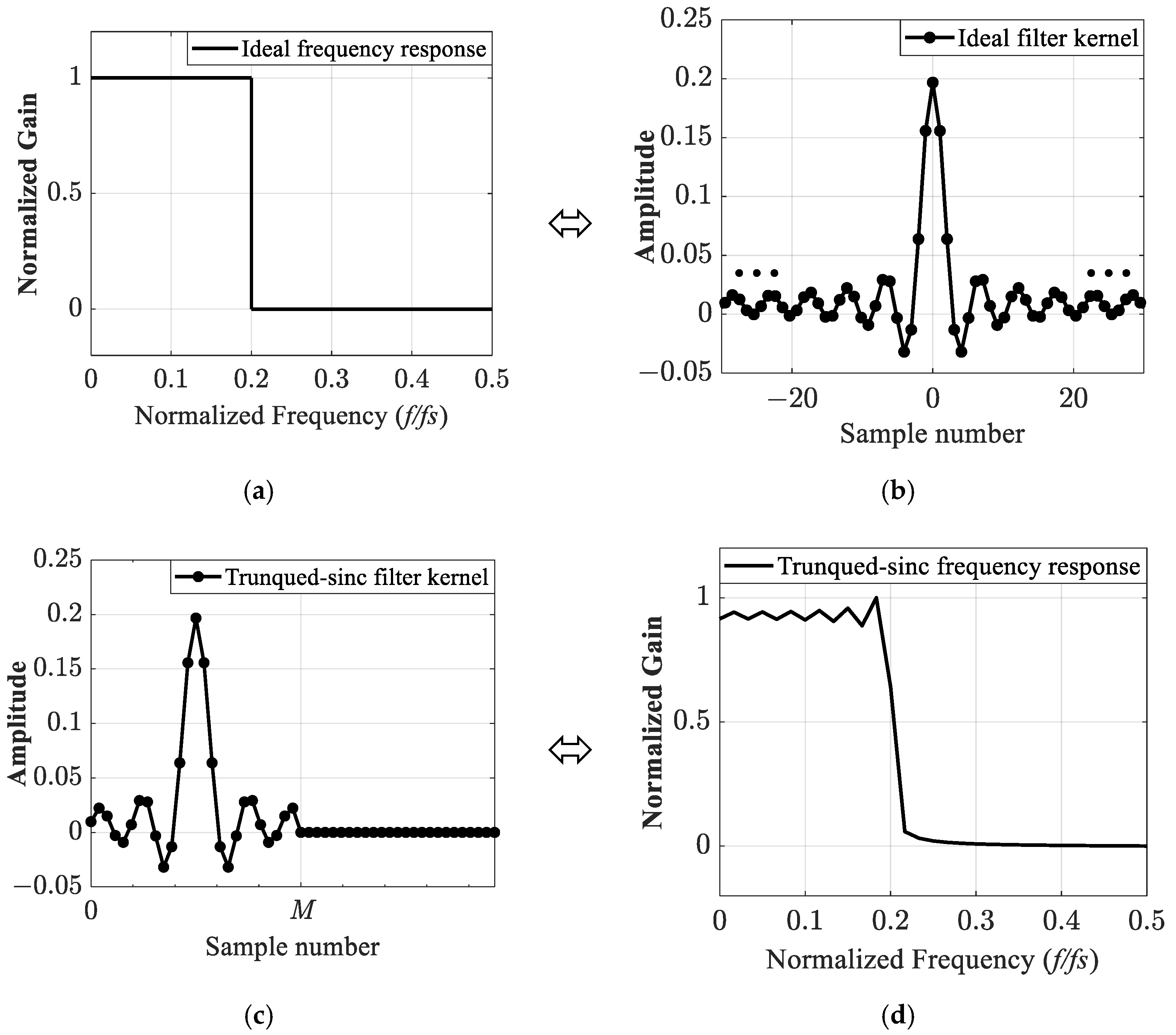
To understand how a window digital filter is obtained, one must start from the ideal filter response in the frequency domain. The kernel of the ideal frequency-domain filter is a rectangular function (Figure 1a), and its time-domain equivalent is a sinc function (Figure 1b), which is obtained by the inverse Fourier transform of the rectangular function. The idea is to give unity gain to the components of interest in the signal, and to give zero gain to the other components. This is accomplished by multiplying the kernel by the signal in the frequency domain, or convolving them in the discrete time domain, as seen in (2).

For sinc kernel to be implemented in a computer, that is, in a discrete domain, the sinc function must be limited (truncated) symmetrically around the main lobe, with M + 1 points (M must be an even number, and the sum of one is due to the central symmetry point), and all samples outside this range must be set to zero [24]. Also, the entire sequence must be shifted to the right so that the kernel can “run” from zero to M, resulting in a causal function (Figure 1c). However, the abrupt discontinuities at the ends of the truncated sinc result in unwanted ringing at the band-pass and overshoot around the cutoff frequency (Figure 1d). This distortion phenomenon is known as the Gibbs effect [15,24].

A very efficient method to reduce the distortions in the frequency domain is to multiply the truncated sinc by a weighting function, known as the apodization window (hence the name of the windowed-sinc filter). Thus, the apodization window makes the ends of the sinc function gradually decrease to zero.

There is a variety of apodization functions, but the Hamming and Blackman windows are particularly advantageous as they have higher stopband attenuation than others. While the stopbands of the rectangular (windowless), Bartlett (triangular), and Hanning (raised cosine) windows are −21 dB, −25 dB, and −44 dB, respectively, the Hamming and the Blackman windows are −53 dB and −74 dB, respectively. On the other hand, the roll-off of the Blackman window is 3 times larger than the roll-off of the rectangular window and 1.5 times larger than that of the Hamming window. Moreover, the roll-off rates are the same Hanning and Bartlett windows [15]. Therefore, for a given kernel of length M + 1, the choice of an apodization window is a trade-off between stopband and roll-off.

Although the stopband is dependent on the window type, the roll-off can be adjusted by increasing or decreasing M: the larger the M, the faster the roll-off, and vice versa [24]. This means that a Blackman window could achieve the Hamming roll-off while maintaining the Blackman stopband, but the filtering computing time also increases due to the convolution operation (2).

2.3. Band-Pass Filter with Hamming Window and Blackman Window

The Hamming window (HW) and the Blackman window (BW) filters were used in this work because they have larger stopbands than the other window filters mentioned here. The process for designing the two filters is very similar, so they were designed together in this section. A band-pass filter is suitable to improve the characterization of the acoustic field, as the transducer bandwidth has been previously characterized using the pulse-echo measurement. By fitting the frequency band of the band-pass filter within the bandwidth of the transducer, the pulse is separated from unwanted noise in the sampled window measured with the hydrophone.

In the design of a filter, the lower and upper cutoff frequencies (respectively, f₁ and f₂) must be normalized by the sampling frequency, f_s, and must be a value between 0 and 0.5 [24] (considering the Nyquist frequency).

The value of M must be an even positive integer. It can be approximated by [24]

$$M=\frac{4}{BW},$$

(3)

where BW is the frequency bandwidth of the roll-off, which is also normalized by the sampling frequency f_s. Equation (3) is a trade-off between the roll-off speed and computation efficiency: the larger the M, the faster the roll-off (because the transition bandwidth is shorter) and the longer the computation time is, and vice versa.

Afterward, the kernel of the windowed-sinc Hamming filter was calculated by [24]

$$h\left[i\right]=k\left[\frac{\sin \left(2\pi f_2\left(i-\frac{M}{2}\right)\right)}{i-\frac{M}{2}}-\frac{\sin \left(2\pi f_1\left(i-\frac{M}{2}\right)\right)}{i-\frac{M}{2}}\right]\left[0.54-0.46\cos \left(\frac{2\pi i}{M}\right)\right].$$

(4)

In (4), the arguments of the sinc functions, which are inside the left brackets, are subtracted by −M/2 to shift them to the right (see Figure 1c). In order to avoid division by zero when i = M/2, then the equation h[M/2] = k (2π f₂ − 2π f₁) is used to replace Equation (4). The k is constant for a unity gain filter. In practice, k is disregarded while the kernel is being computed and then all samples are normalized as needed [24]. This can be conducted by normalizing the kernel FFT, and the kernel filter is obtained by applying the inverse of the FFT.

The Blackman window filter is obtained by replacing the expression inside the right brackets of (4), which is a Hamming window function, with the Blackman window function, as shown here [24]:

$$h\left[i\right]=k\left[\frac{\sin \left(2\pi f_2\left(i-\frac{M}{2}\right)\right)}{i-\frac{M}{2}}-\frac{\sin \left(2\pi f_1\left(i-\frac{M}{2}\right)\right)}{i-\frac{M}{2}}\right]\left[0.42-0.5\cos \left(\frac{2\pi i}{M}\right)+0.08\cos \left(\frac{4\pi i}{M}\right)\right].$$

(5)

3. Materials and Methods

In this section, the acoustic field measurement and simulation processes, as well as the design of the filters and performance evaluation, are presented.

3.1. Quantitative Analysis

The pure qualitative analysis of the results regarding waveforms and acoustic fields can lead to misinterpretations, as the perception of the results is subjective [13]. Thus, to obtain accurate comparisons, the filter performance was numerically calculated by using the root mean square error (RMSE) equation [25]:

$$RMSE=\sqrt{\frac{1}{N}\sum _{i=1}^N{\left({AF}_{SIM}\left[i\right]-AF\left[i\right]\right)}^2},$$

(6)

where AF_SIM are the simulated values (gold-standard reference), AF are the measured values (not filtered, and filtered), i is an index of the sample of a pulse or a given point (x, z, y = 0) located at the acoustic field, and N is the number of samples or points of the respective measurement.

To quantify the point-to-point absolute error between the filtered and the gold-standard acoustic fields, the absolute error (AE) was used as a metric. This index of quality allowed comparisons of the acoustic fields by using images of errors. An error image is an image that attributes a color to a given AE[i], which was calculated by [26]

$$AE\left[i\right]=\left|{AF}_{SIM}\left[i\right]-AF\left[i\right]\right|$$

(7)

3.2. Acoustic Field Measurement

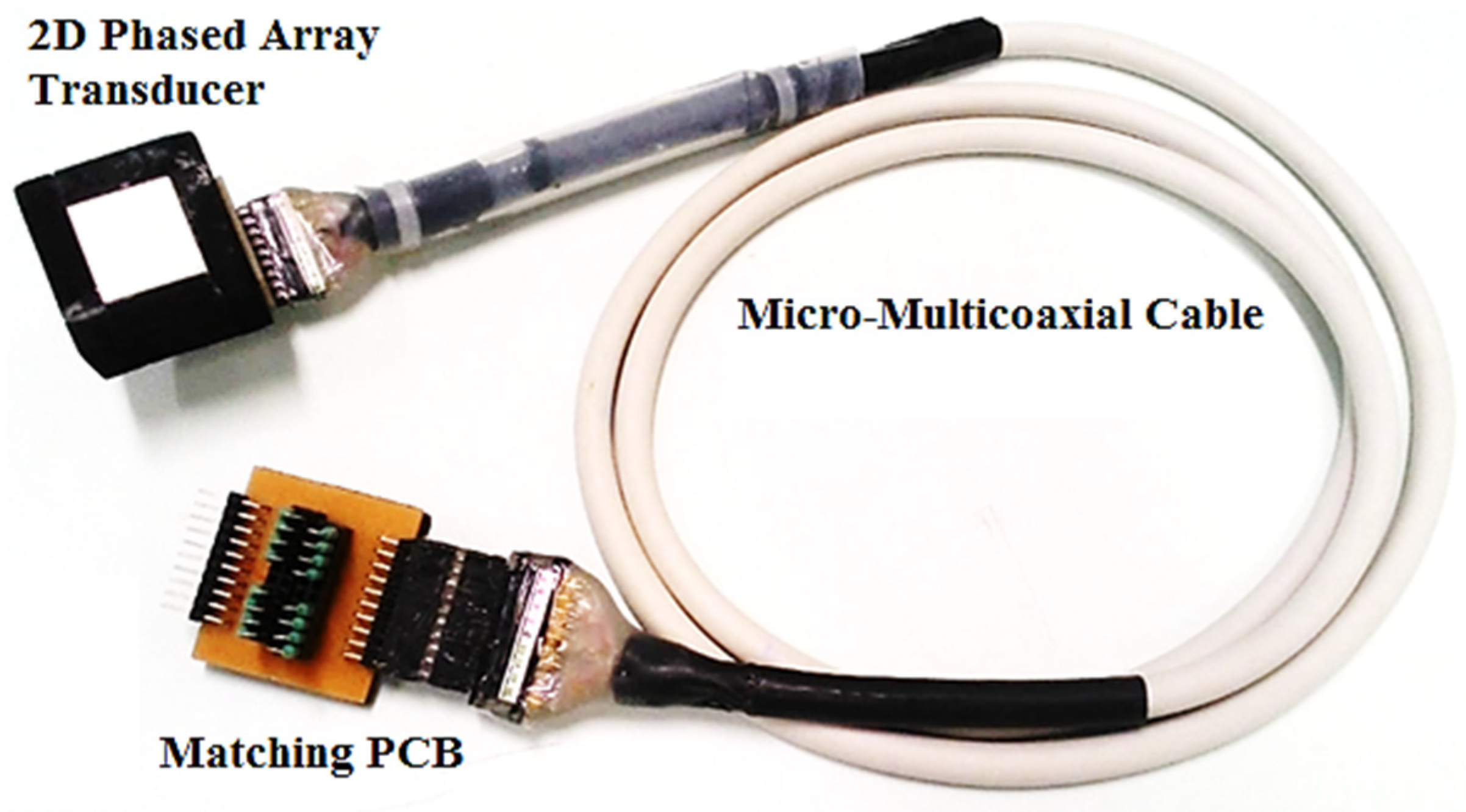
The acoustic field from a 2D phased-array ultrasound transducer (Figure 2) was measured with the self-made needle hydrophone described in [5]. Because the hydrophone was not calibrated, the measurements were normalized by the maximum amplitude of the field. The phased-array transducer used in this work is the same transducer used in [27] to make 3D acoustic images of objects immersed in water. The transducer consists of 16 squared elements with sides equal to 5 mm distributed in a 4$\times$4 matrix, which can emit and receive ultrasound pulses individually. The center frequency of the transducer is 480 kHz and its −6 dB bandwidth is 50% [27]. Both the transducer and the hydrophone were built in our ultrasound laboratory.

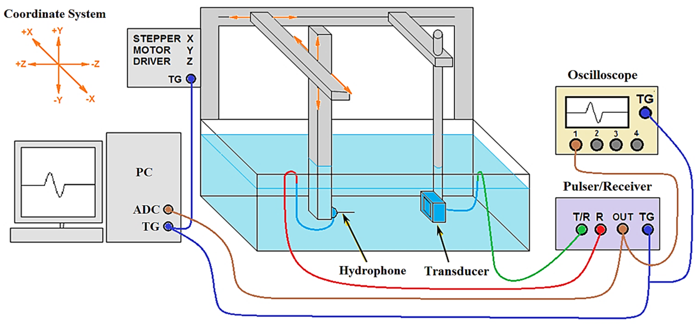
The transducer was excited by an ultrasonic pulser/receiver (5077PR, Panametrics-NDT, Waltham, MA, USA), which was adjusted to a 500 kHz squared pulse with an amplitude of 100 V, 10 dB gain, and a 10 MHz low-pass filter. The acoustic field generated by the transducer was measured in a water tank (Figure 3), with a needle hydrophone held by an automatic scanning system, sweeping the xz-plane at y = 0.

As the pulser/receiver has only one T/R channel; all the transducer elements were connected in parallel, emitting at the same time. Thus, the measured acoustic field was equivalent to that of a single-element square transducer with a 20.6 mm side.

The ultrasonic pulse emitted by the transducer reached the hydrophone at an x, z point in the field. Consequently, the hydrophone generated an electrical pulse that was received by the R channel of the pulser/receiver, which filtered the signal with a 10 MHz analog low-pass filter. This frequency was 20 times greater than the central frequency of the transducer.

The digital oscilloscope (MSO8104A Infiniium, Agilent Technologies, Englewood, CO, USA) was only used for the transducer–hydrophone alignment process, which consisted of moving the hydrophone in front of the transducer surface. This was necessary to define the position of the center of the transducer and to adjust the scanning system.

Next, the pulser/receiver sent the pre-filtered signal for its digitization, which was performed on an 8-bit analog-to-digital converter (ADC) board that had a maximum sample rate of 100 MS/s (NI PCI-5112, National Instruments, Austin, TX, USA). In order to reduce the amount of data for processing, the signals were sampled at 25 MS/s. The digitization frequency was 2.5 times higher than the analog low-pass filter. Therefore, the Nyquist criterion was observed to avoid undersampling.

After digitalizing and storing the signal in the PC, it sent a synchronized trigger pulse to the tank driver to move the hydrophone with a step of 1 mm (λ/3) in z; when the z-axis was fully swept, the hydrophone was moved with a step of 1 mm in x and the path of z was reversed. The process was repeated until the entire plane −50 mm ≤ x ≤ 50 mm by 5 mm ≤ z ≤ 150 mm was sampled.

Before the acoustic field calculation, the DC components in the signals were removed by subtracting the mean. Then, the acoustic field was obtained in MATLAB (The MathWorks, Inc., Natick, MA, USA) by assigning to each point of the mesh the maximum pulse amplitude at its respective point. Finally, the measured acoustic field was normalized.

3.3. Acoustic Field Simulation

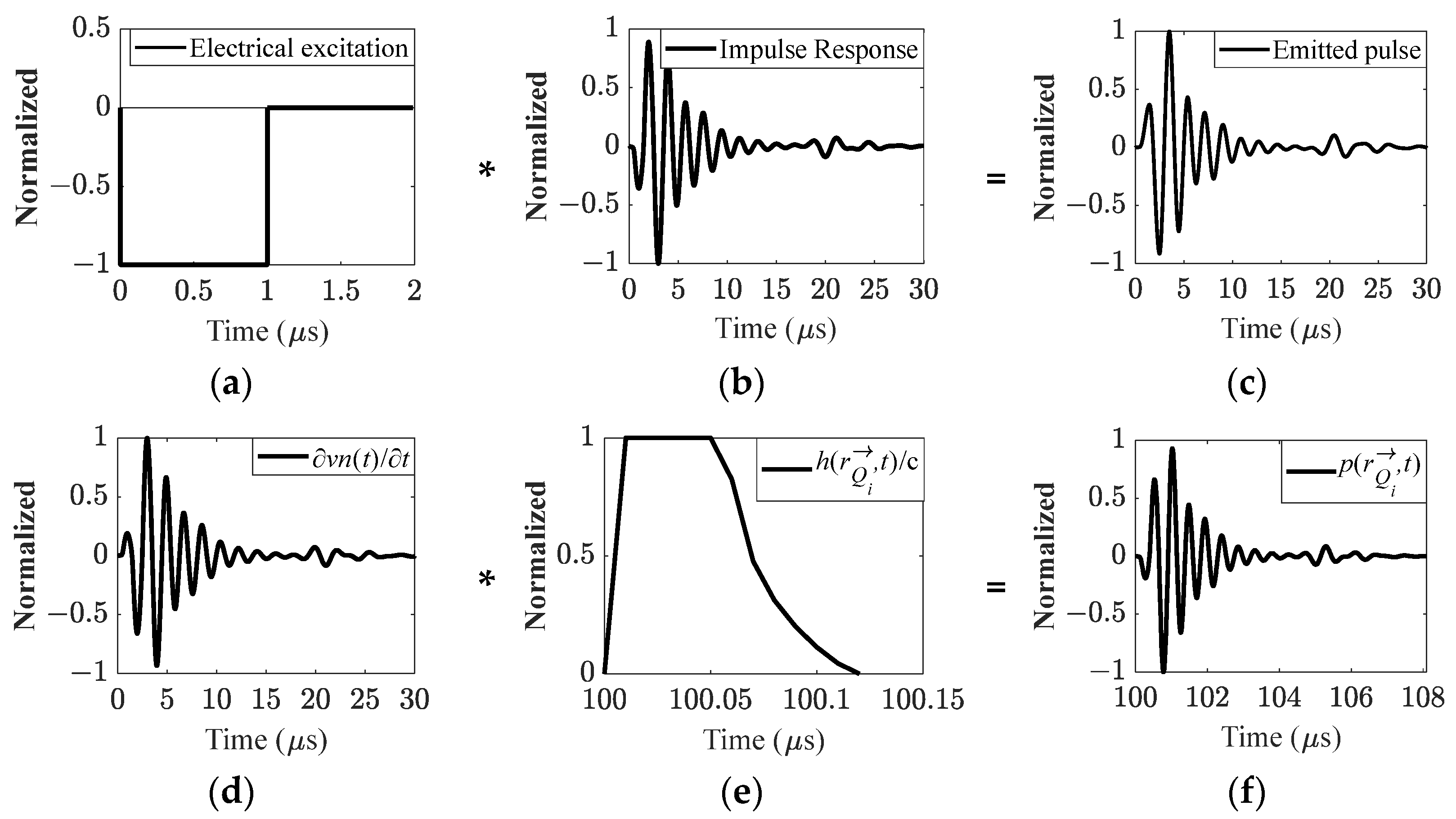
The steps taken to simulate the acoustic fields in MATLAB are presented in Figure 4. First, a pulse emitted by the transducer, called vn(t), was obtained using the modeling of the KLM and ABCD matrices (Figure 4a–c) [28,29,30]. Then, the pressure wave p(${\overrightarrow{r}}_Q$,t), at a spatial point Q in the field, was calculated with the rigid-plane piston model, where ${\overrightarrow{r}}_Q$ is the position vector of the point Q (Figure 4d–f) [25,31,32]. This linear model describes a piezoelectric transducer as a piston in which the face particles vibrate in a phase, with velocity vn(t), normal to the transducer face. The acoustic field at a position Q is the maximum amplitude of p(${\overrightarrow{r}}_Q$,t). The model used in the simulation was accurate for the purpose of the experiment, considering that the medium for measuring the acoustic field is water, which meets the boundary conditions of the model, because it is homogeneous and isotropic.

The developed algorithm took into account all parts of the transducer presented in Figure 2, such as piezocomposite elements, matching layer, backing layer, and also the micro-multicoaxial cable and series inductors, used to match the electrical impedance of the transducer with that of the pulser/receiver.

In addition, a squared negative electrical pulse (Figure 4a), similar to that generated by the pulser/receiver, was used for transducer excitation. It was possible to simulate a pulse with the same characteristics as the real transducer, a central frequency f_o of 480 kHz and 50% bandwidth (Figure 4c), making the simulation of the acoustic field more accurate.

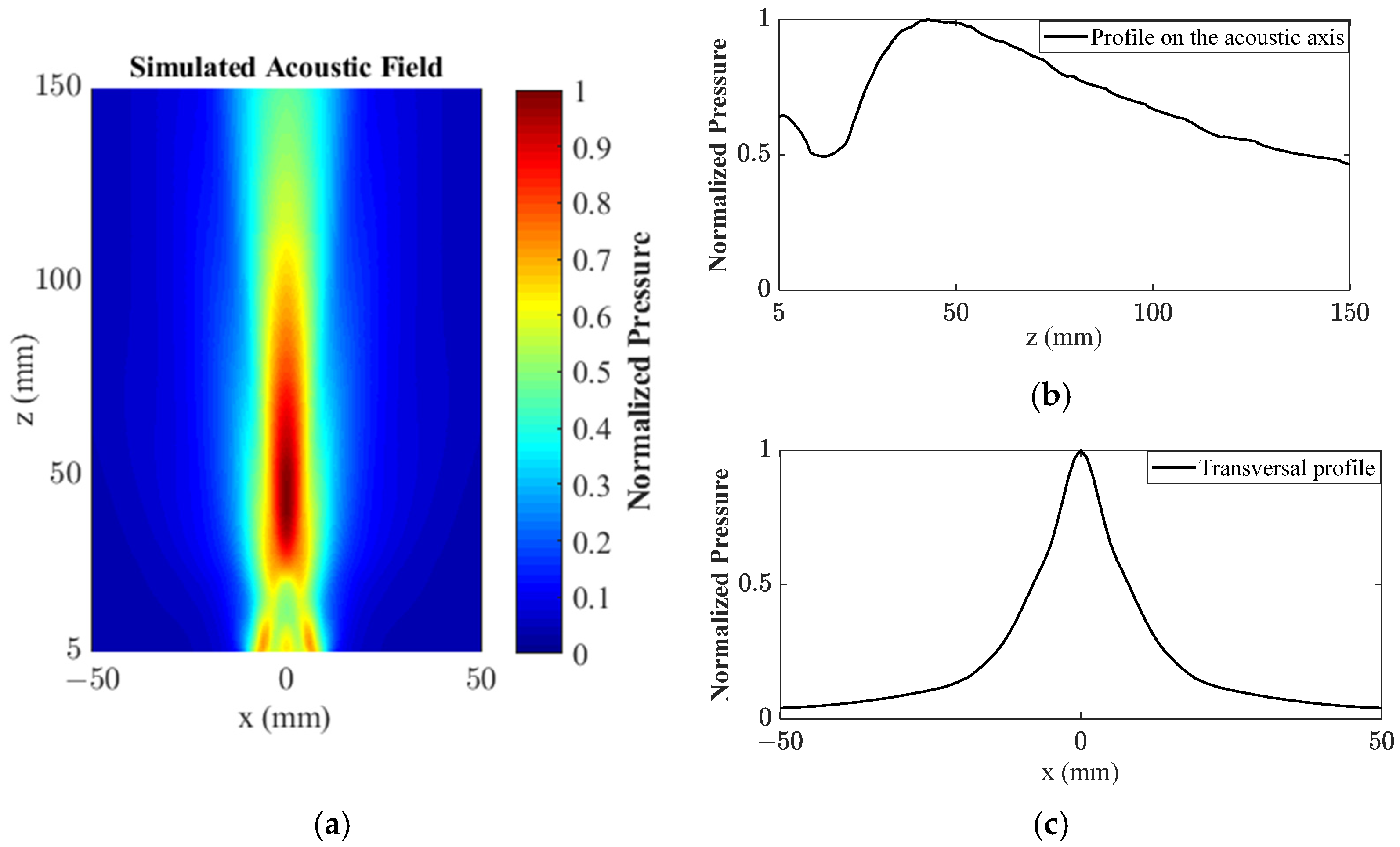
Moreover, parameters such as the grid size and its discretization, as well as the sampling frequency used to simulate the acoustic field, were equal to those used in the measurements. The ultrasound propagation velocity in water was c = 1500 m/s. The noise was disregarded in the pulses. Figure 5 shows (a) the acoustic field simulated at the xz-plane, (b) its axial beam profile, and (c) its lateral beam profile. The acoustic pressure along the acoustic axis (z-axis) is useful for determining the focal distance where the amplitude is maximum. The lateral beam profile at the focal distance is useful for determining the lateral resolution, given as the full-width at the half-maximum (FWHM).

3.4. Design of the Moving Average Filter

The length of the MA kernel, M, was varied, and the MA filter was applied to the noiseless simulated pulse (Figure 4) to analyze how it was distorted as a function of M. This was carried out by calculating the RMSE (6) of the filtered pulse with a given M, relative to the simulated pulse.

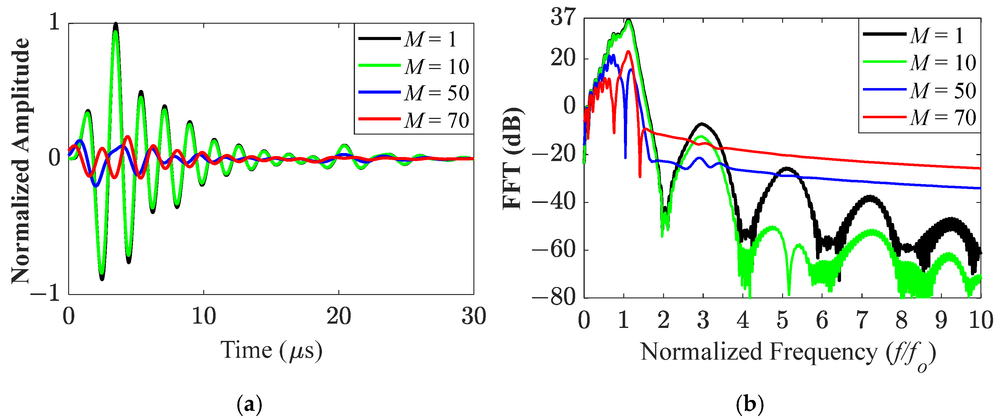
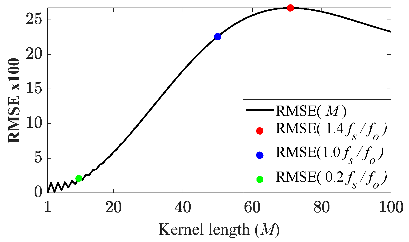
The method was started by applying the MA filter to the simulated pulse, with M from 1 (no filter) to 100 (approximately twice the number of samples of a one-cycle sinusoid at the central frequency of the transducer, f_o, such that M = 2 f_s/f_o) in steps of 1 (for better visualization, only M = {1, 10, 50, 70} pulses are shown in Figure 6). Then, the RMSE was calculated for each filtered pulse (Figure 7). The simulated unfiltered pulse was the reference to calculate each RMSE(M).

This method was useful for choosing an M that would not significantly deteriorate a filtered pulse, as shown in Figure 6a and Figure 7. The larger the kernel of the MA filter, the more uncharacterized the pulse was.

In turn, a shorter kernel could preserve the waveform while attenuating high frequencies, as shown in Figure 6a,b, respectively. This suggests that, although the MA filter acts as low-pass filter, care must be taken to choose a kernel length so as not to mischaracterize the pulse. After testing different kernel lengths, it was found that M = 0.2 f_s/f_o was a suitable kernel length for the MA filter, as the RMSE when M = 10 was only 2%.

3.5. Design of the Hamming Window and Blackman Window Band-Pass Filters

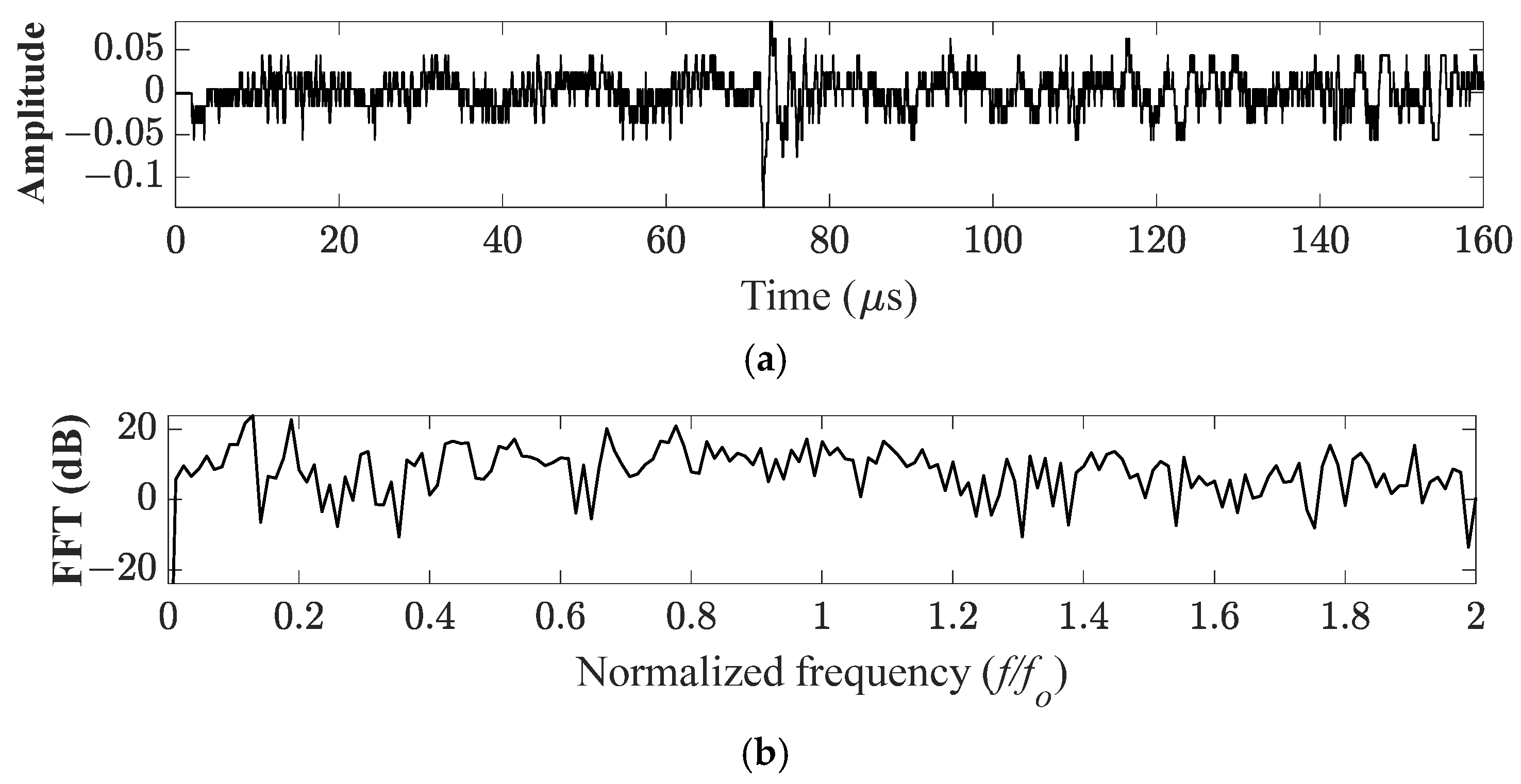
While the MA kernel filter was designed with a simulated pulse, the window filters were modeled using a measured signal. The pulse was measured at x = 25 mm, z = 100 mm, far off the acoustic axis, in the far field, and normalized by the highest of all measured pulses in the acoustic field.

This point was chosen because it was possible to locate the pulse emitted by the transducer (see Figure 8a, between 70 µs and 80 µs) as well as unwanted noise and oscillations. The oscillations that are evident below 70 µs have a frequency lower than that of the pulse emitted by the transducer. Averaging the measurements can indeed remove random noise. However, it was not possible to average the results because it would considerably increase the time for acquisition. The signal acquisition was automatic, i.e., the signals were continuously acquired while the hydrophone swept the field.

Applying the FFT to the signal, frequency components outside the transducer operating range (0.75 f_o to 1.25 f_o) were identified with magnitudes comparable to and even greater than those of the transducer operating, as noted at 0.12 f_o and 0.2 f_o in Figure 8b. The amplitude of the high-frequency noise was slightly lower than that of the pulse, but the duration of the low-frequency noise was longer than that of the pulse. As a consequence, the energy of the noise and oscillations was comparable to that of the pulse, making it impossible to identify its effective range in the frequency domain presented in Figure 8b.

In order to attenuate unwanted frequencies and, at the same time, not to mischaracterize the measured pulse of the transducer, the low and high cutoff frequencies of the band-pass filter were f₁ = 0.25 f_o (120 kHz) and f₂ = 1.50 f_o (720 kHz), respectively.

The transition band between the cutoff frequency and the stopband was chosen as BW = 0.10 f_o (48 kHz), resulting in M = 2084 (3) (considering that BW must be normalized by f_s, and M is an even number). The transducer operating band was, thus, kept within the band-pass filter band.

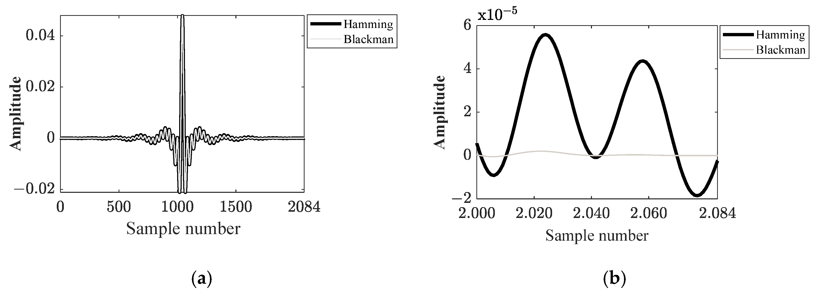
After calculating the kernel size, the kernels of the Hamming window filter and of the Blackman window filter were calculated using Equations (4) and (5), respectively.

Although the kernels look very similar (Figure 9a), the Blackman kernel truncation was smoother than the Hamming kernel truncation (Figure 9b), which can reduce ringing in the band pass range and reduce overshoot near the cutoff frequencies.

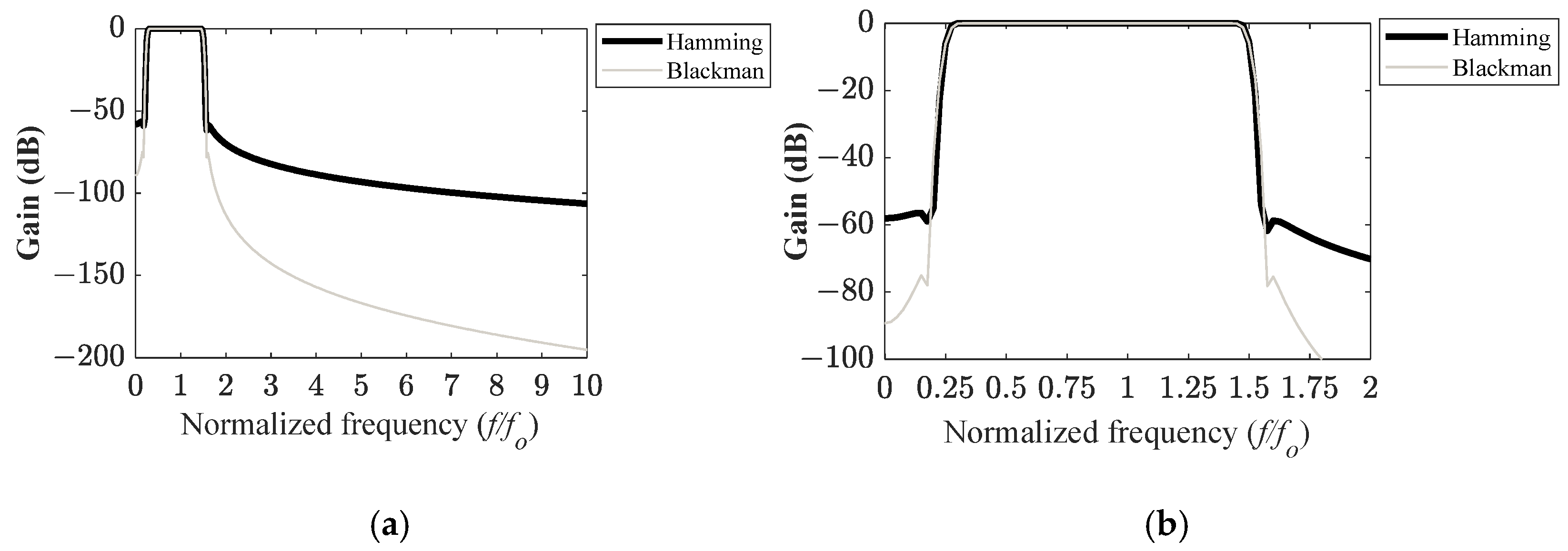
The frequency response of the band-pass filters showed that the Blackman window filter increased attenuation out of the band-pass range more than the Hamming filter does (Figure 10a). The Blackman window stopband magnitude was lower than that of the Hamming window, and the roll-off from both filters was similar (Figure 10b).

4. Results

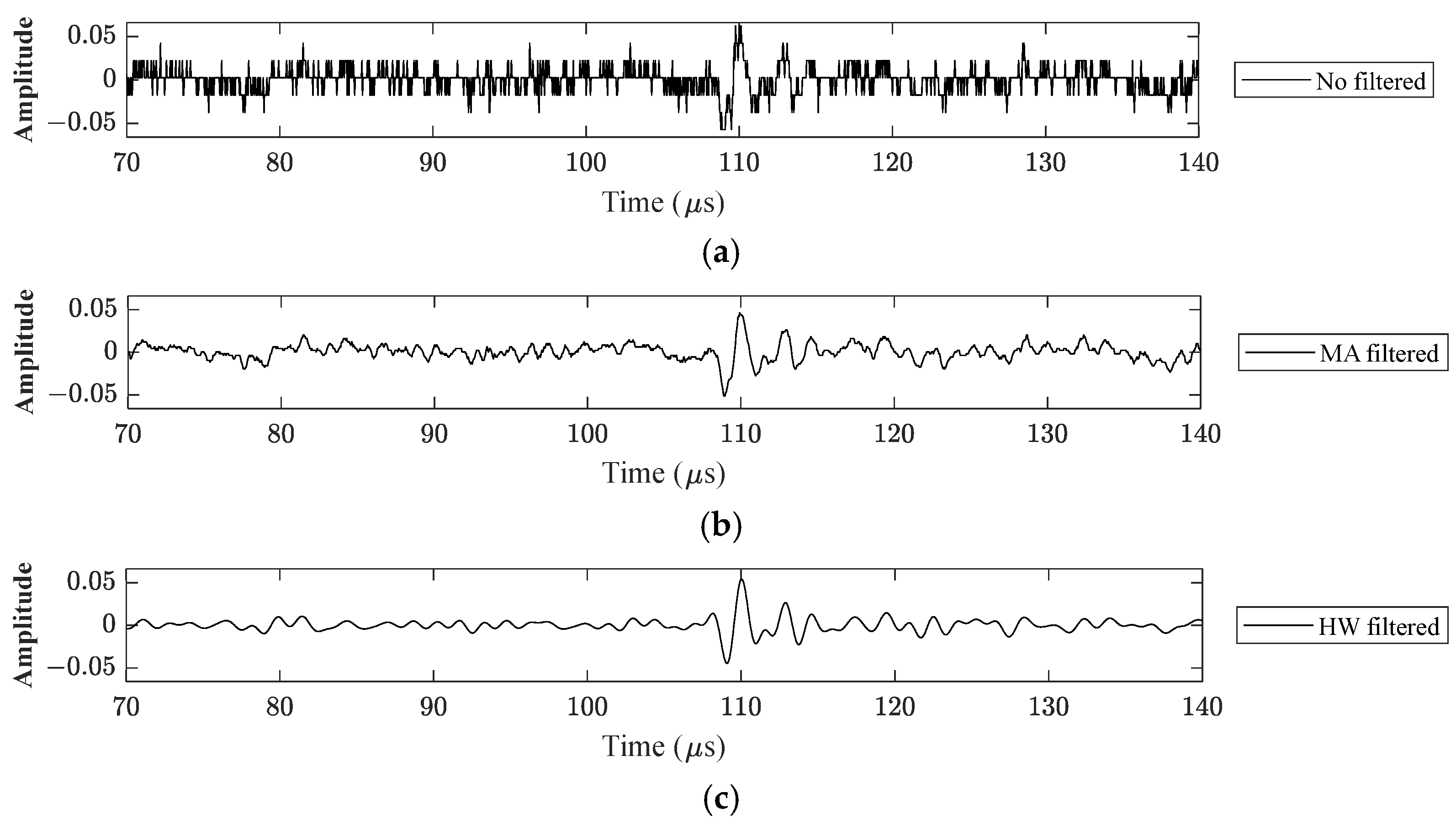
To evaluate the performance of the filters, a pulse was measured at x = 50 mm, z = 150 mm in the plane y = 0, normalized by the maximum amplitude of the field. The location chosen to acquire the signal is critical because its amplitude is greatly attenuated off the acoustic axis and in the far field, making the pulse and noise magnitudes comparable (Figure 11a). Thus, a noise could be computed as a pulse, generating an error in the determination of the acoustic field. Although the signal was limited by the 8-bit acquisition board, it was able to show that the filters actually work.

Although the MA filter with M = 10 smoothed the signal, unwanted distortions remained, with significant amplitudes around 80 µs, and from 117 µs (Figure 11b). The same MA filter applied to the simulated pulse of Figure 6a made the attenuation significant from 2 f_o on. Thus, it is reasonable to consider that the signal was smoothed when the high frequencies were filtered, and that the remaining disturbances were at frequencies in the operating range of the transducer and below that.

In turn, the HW (Figure 11c) and the BW (Figure 11d) window filters with M = 2084 were more effective than the MA filter, as they make it easier to identify the pulse around 110 µs. The frequency response of the filter kernels modeled in Figure 10 showed that frequencies below 0.25 f_o and above 1.50 f_o were greatly attenuated; one may hence assume that unwanted distortions remain at frequencies around the operating band of the transducer.

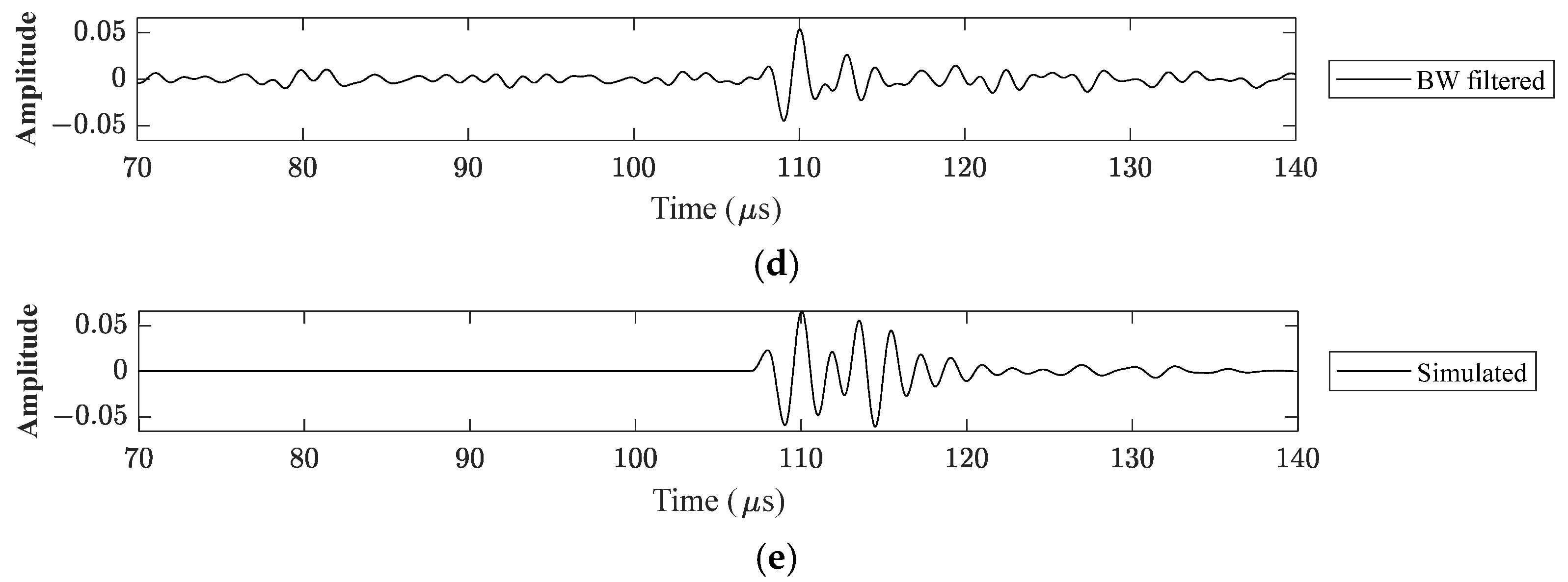
However, comparing the pulses filtered with HW (Figure 11c) and BW (Figure 11d) with the simulated noiseless pulse (gold standard—Figure 11e), some noise was removed. This suggests that unwanted frequency components are also included in the operating band of the transducer, and that the linear filters in this work cannot remove them.

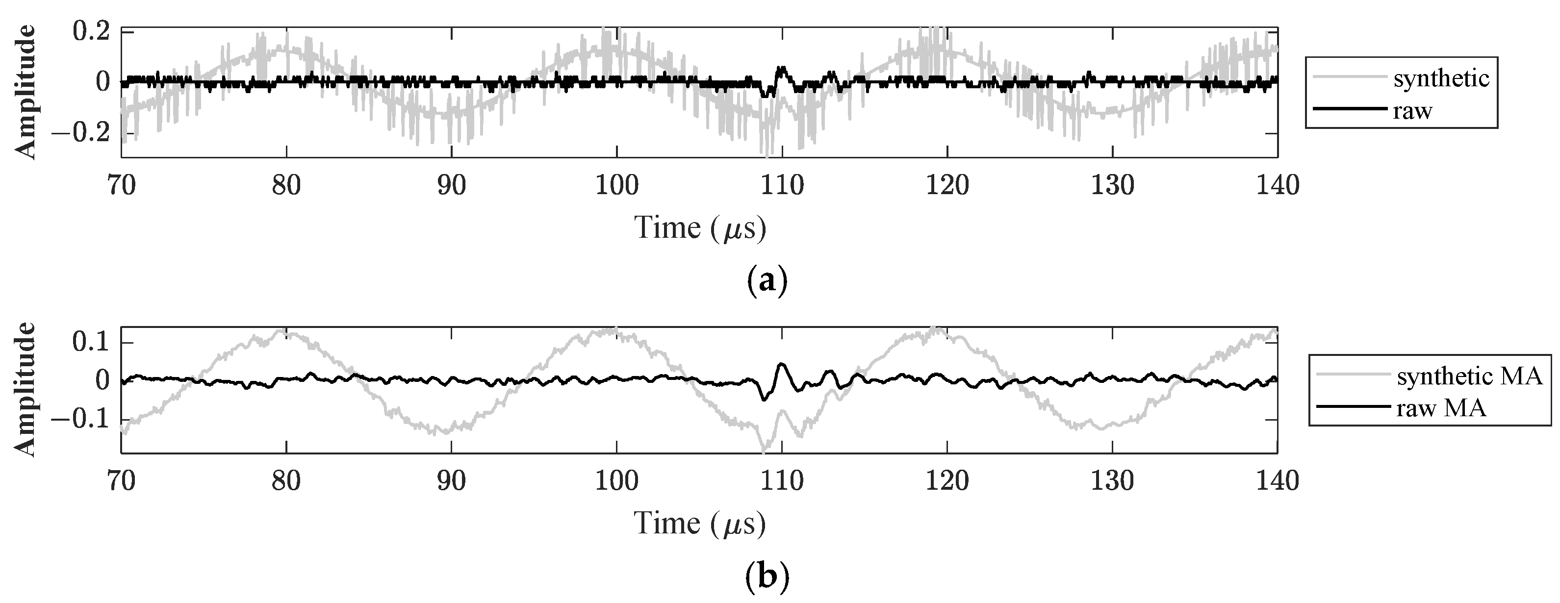
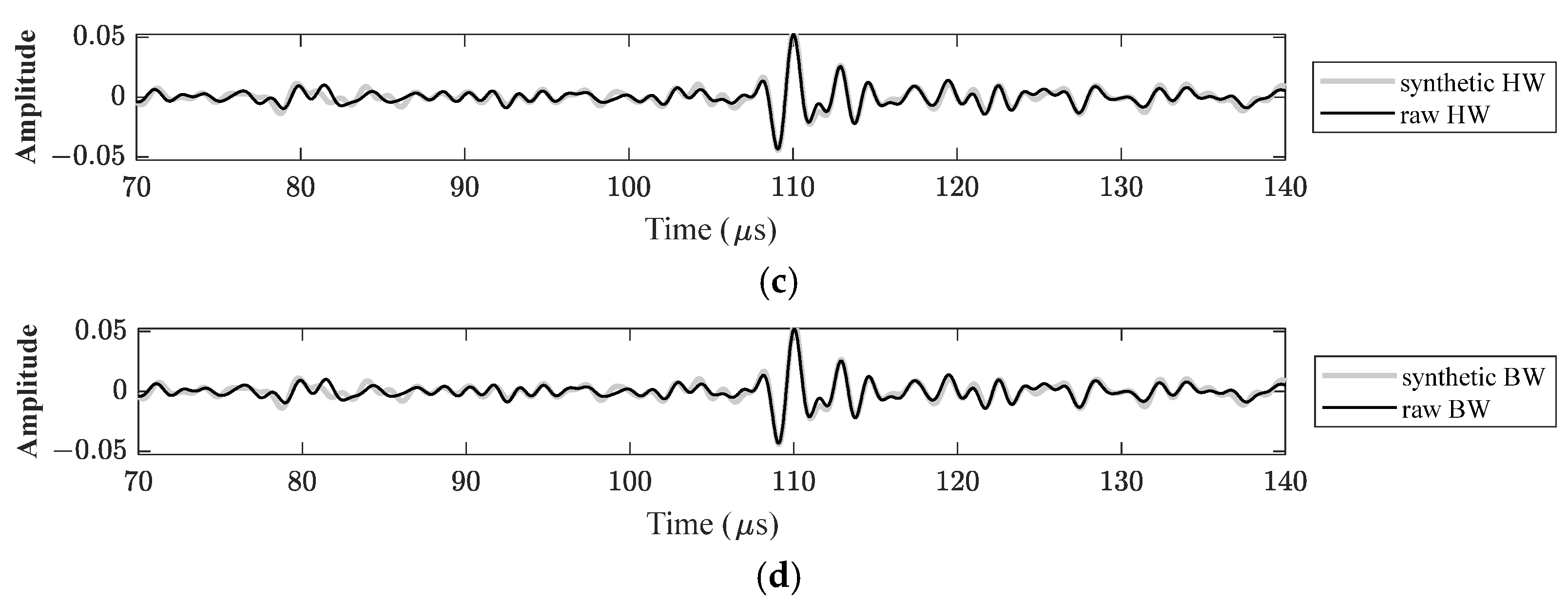
The filtering of high-amplitude noise was evaluated by adding a synthetic noise, simulated in MATLAB, to the measured signal presented in Figure 11a. The synthetic noise was the result of the sum of a 50 kHz continuous wave and 200 random pulses (single-sinusoidal cycles of 10 MHz), both with twice the maximum amplitude of the measured signal.

The 50 kHz continuous wave was low-frequency noise and the 10 MHz random pulses were high-frequency noise. The unfiltered measured signal (raw) is shown in Figure 12a, and the same signal with synthetic noise (synthetic), before and after MA, HW and BW filtering, are shown in Figure 12b–d, respectively.

As in Figure 11b, the MA filter in Figure 12b did not remove the low-frequency noise from the signal with the synthetic noise, but it did smooth out the high-frequency noise. On the other hand, the HW filter (Figure 12c) and the BW filter (Figure 12d) were very effective in removing low- and high-frequency noise.

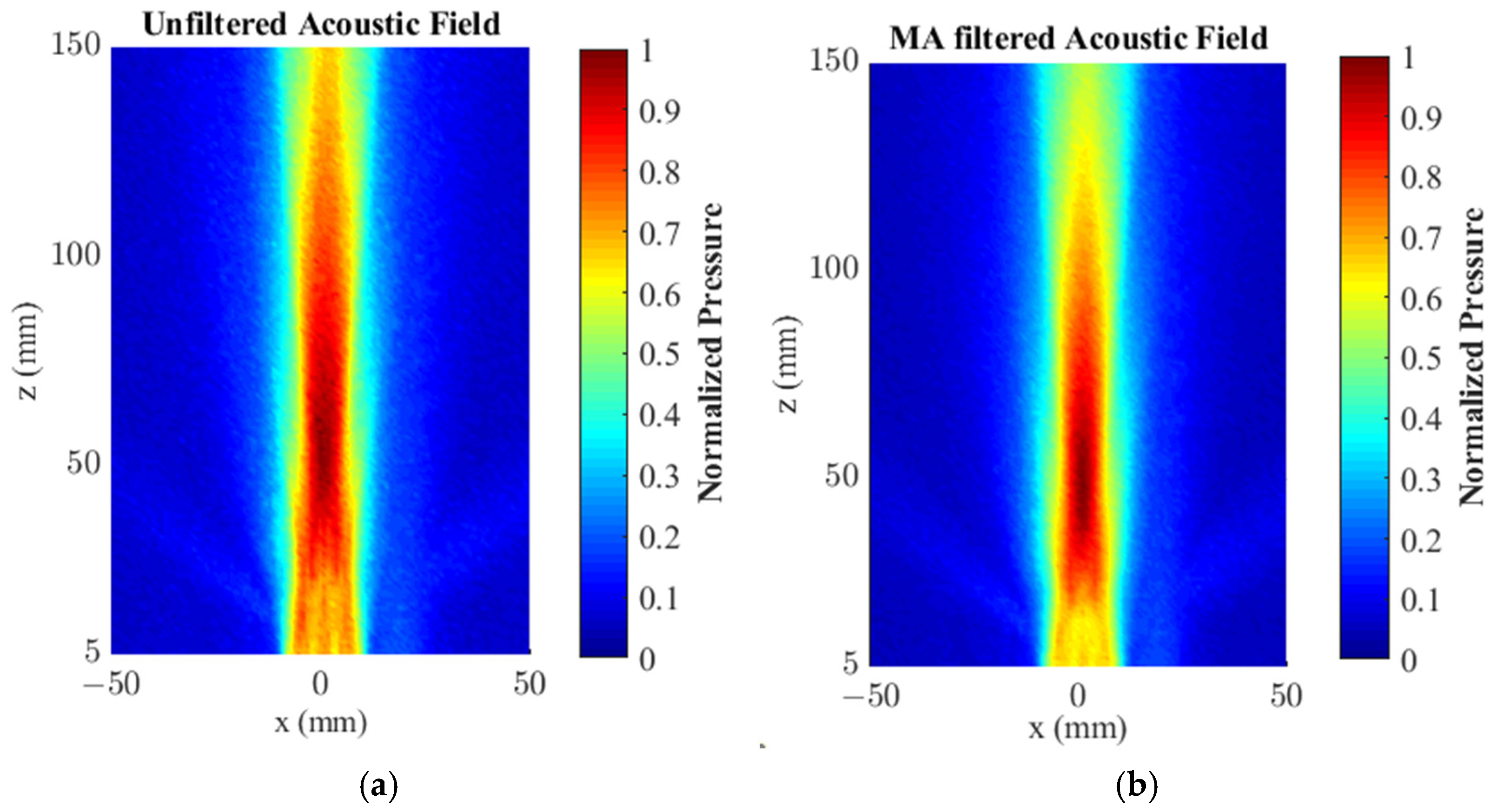
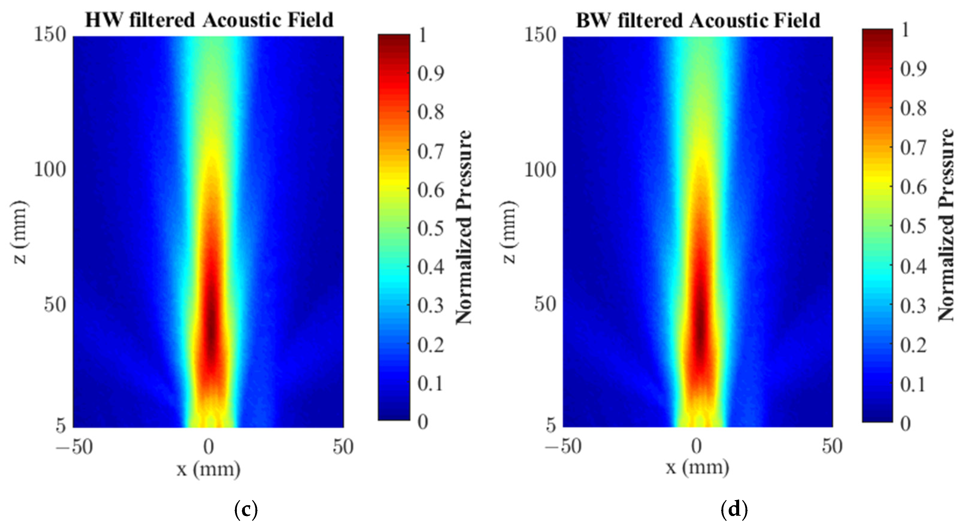
The measured acoustic field (Figure 13a) was filtered by applying the filters MA with M = 10 (Figure 13b), HW with M = 2084 (Figure 13c) and BW with M = 2084 (Figure 13d). The filter kernel was applied in each sampled signal in the mesh, and the pressure at a given x, z point was the maximum of the absolute value over the sampled signal. All values were normalized by their respective filtered acoustic field.

The RMSEs of the measured/filtered acoustic field in relation to the simulated one were 6.34% for the unfiltered, 4.28% for the MA-filtered, and 4.01% for the HW- and BW-filtered acoustic fields. Although the window filters reduced the RMSE by only around 0.27% relative to the MA filter, there was a qualitative improvement when comparing the filtered acoustic fields of Figure 13 with the simulated noiseless one in Figure 5a.

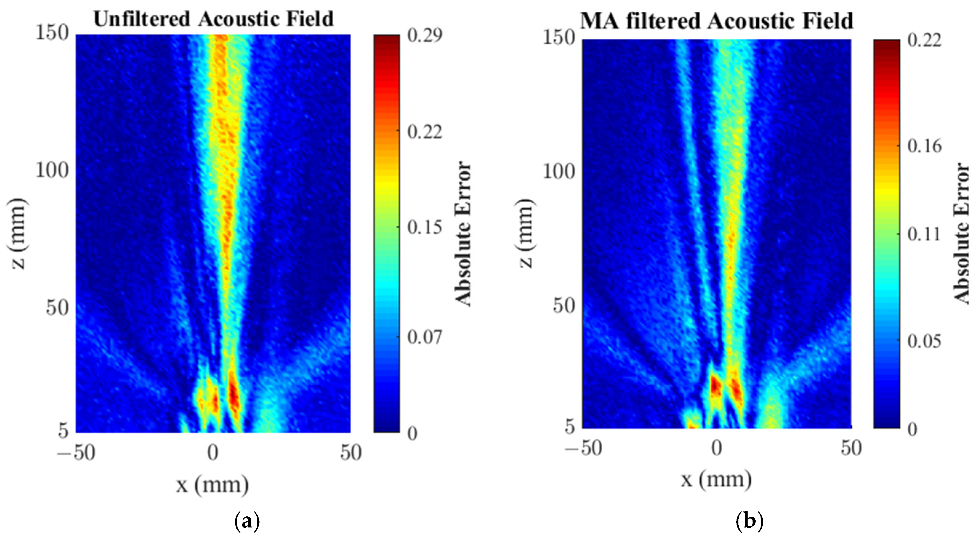
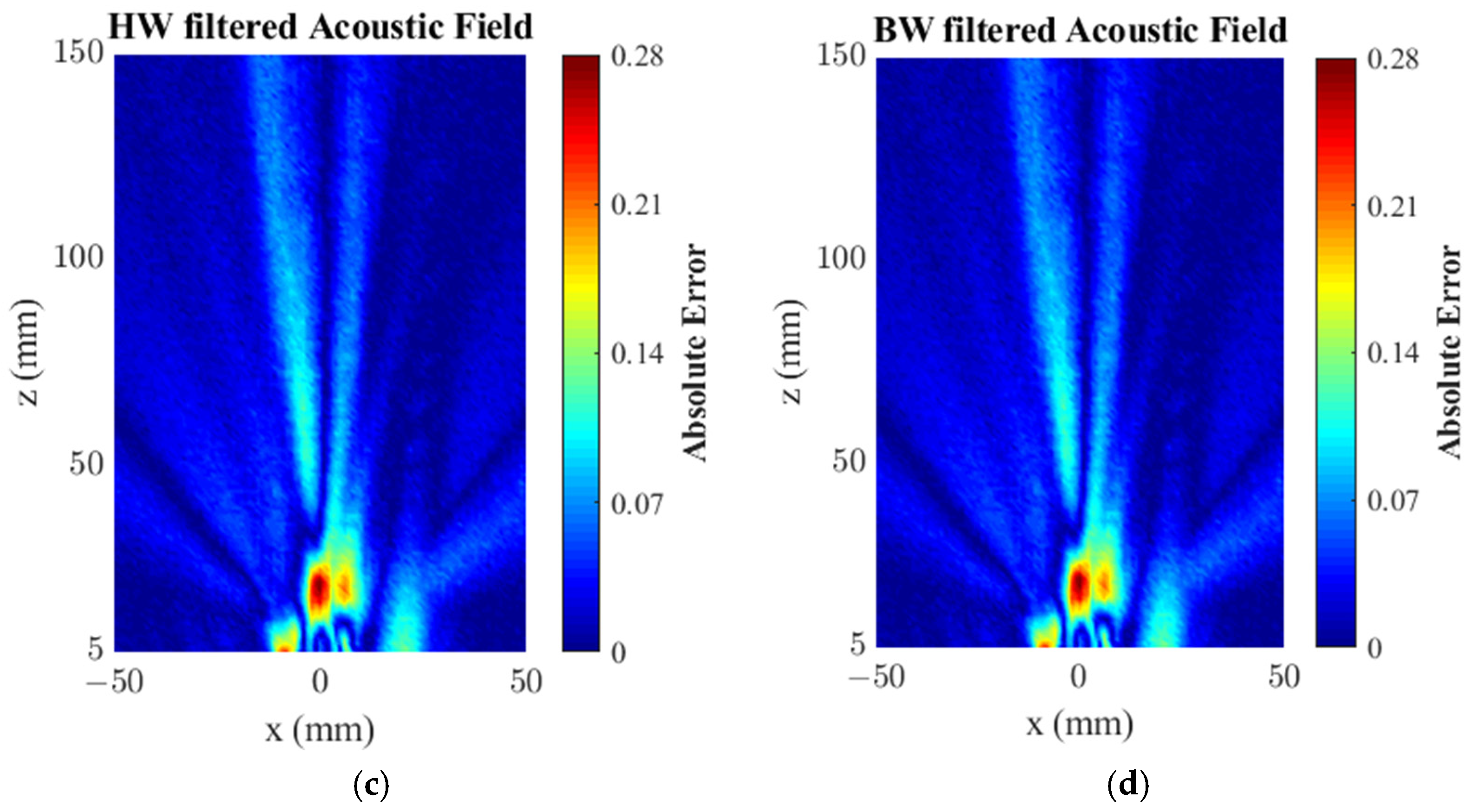
For better visualizing the measured acoustic-field error as well as the performance of the filters, images of the absolute error of the measured and filtered acoustic fields in relation to the noise-free simulated acoustic field are given in Figure 14. By calculating the absolute error AE[i] for each point (7), this figure illustrates how different the normalized pressure at each point was in respect to the gold standard. If there were no errors, the image would be all blue.

Although all the images presented large-amplitude errors in the near field (z < 43 mm), all filters improved the measured acoustic field, being more evident along the acoustic axis (x = 0), where the pressure was higher than in other directions (keeping in mind that all array elements were pulsed at the same time, therefore, without beam deflection). Both the unfiltered (Figure 14a) and the MA-filtered (Figure 14b) acoustic field present a granular aspect, while the acoustic fields filtered with the window filters, HW and BW, present smoother images (Figure 14c,d, respectively). This can be explained by the fact that HW and BW filters were capable of reducing the frequency components below the operating band of the transducer, as shown in Figure 8 and Figure 11c,d. The filters HW and BW showed equivalent error images because their RMSE values were equal to 4.01%.

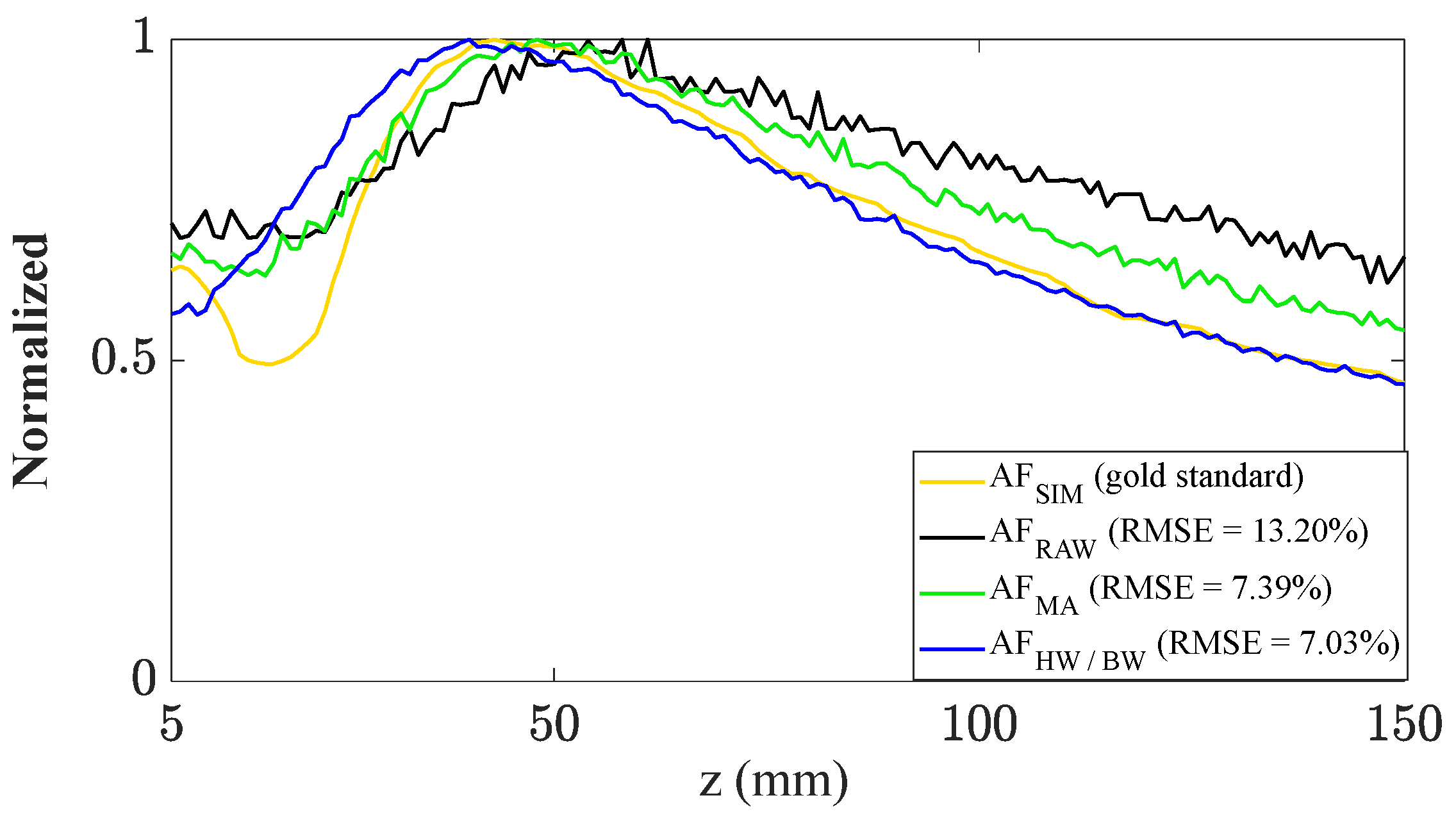
The focal length is the distance from the transducer up to the point where the maximum amplitude occurs, and from which the acoustic amplitude decays monotonically. The axial beam profile showed that the focal length of the measured acoustic field (Figure 15—black line) was further away than the focal length of the simulated acoustic fields (Figure 15—yellow line). The focal length of the simulated acoustic field was 43 mm. The focal lengths of the measured signal were 61 mm for the unfiltered (41.86% further than simulated), 48 mm for MA-filtered (11.63% further than simulated), and 40 mm for the HW- and BW-filtered (6.98% closer than simulated) acoustic fields.

Although this effect could be explained by a measurement error, Figure 15 shows that the focal distance was reduced when a filter was applied to the noised measured acoustic field. Taking into account that the focal distance is frequency-dependent (for a given geometry, the higher the frequency, the longer the focal length) and that the filters applied were low-pass and band-pass filters, the reduction in the focal length can be explained by the attenuation of the high-frequency components of the measured pulses.

In fact, the window filters HW and BW decreased the focal length more than the MA filter (Figure 15—blue line, and Figure 15—green line, respectively), as their higher cut-off frequency was 1.5 f_o, while the MA filter attenuated frequencies higher than 2 f_o (see Figure 6b). In conclusion, the high-frequency noises contributed to an increase the focal length of the measured acoustic field. The RMSE of the normalized pressure profile on the acoustic axis (x = 0 mm, y = 0 mm) were as follows: the RMSE of the unfiltered field = 13.20%, the RMSE of the MA-filtered field = 7.39%, and the RMSE of the HW-filtered and BW-filtered fields = 7.03%.

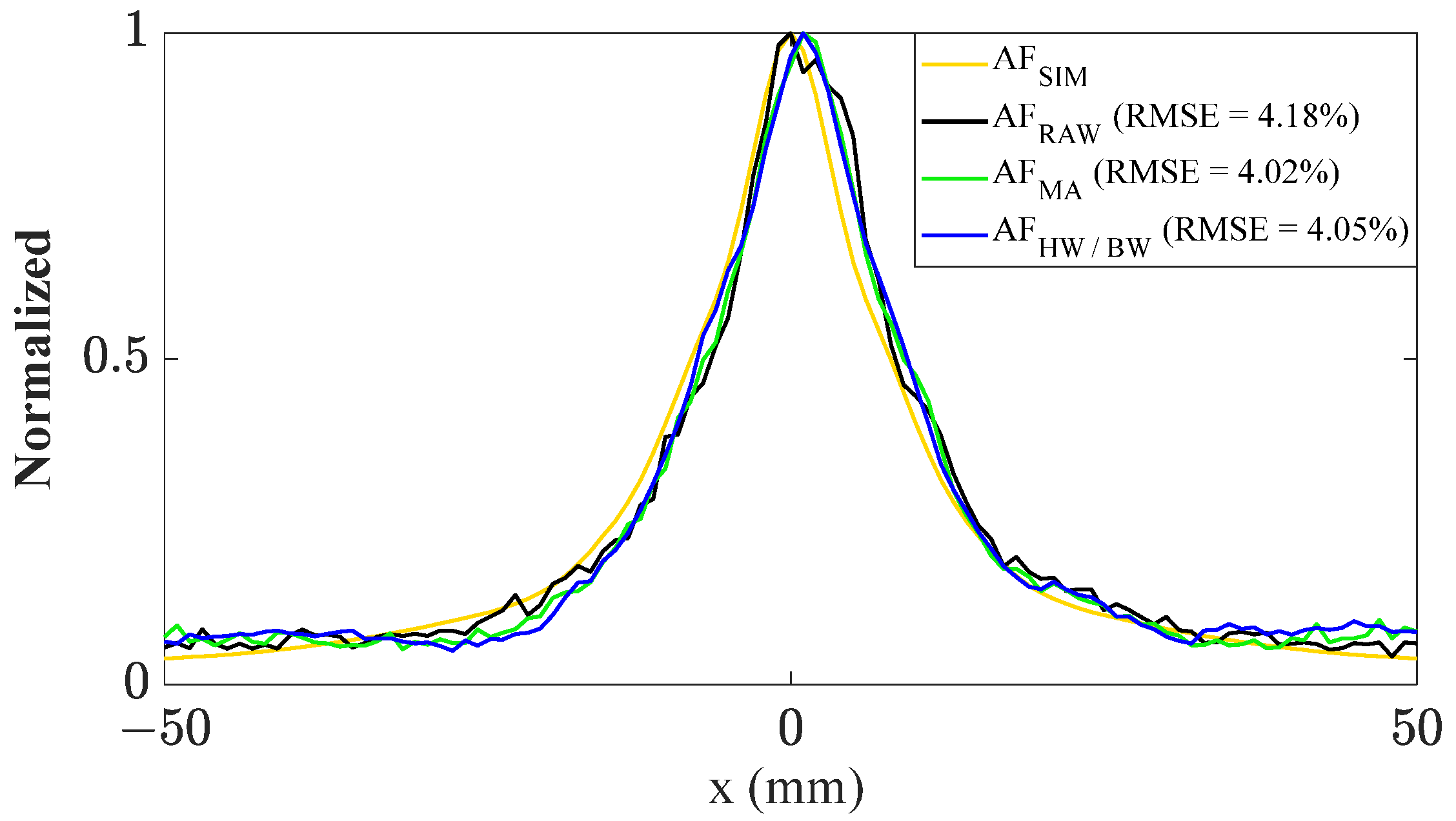
The lateral beam profiles were obtained from their respective acoustic fields (see Figure 13) at their focal points (Figure 16). All the filters improved the results, and the RMSE of the MA filter and of the window filters were equivalent. The filtering performance of the MA, HW and BW filters, summarized in

Table 1. Summary of the main results: RMSE of the measured/filtered acoustic pressure over the entire field, along the z-axis and transversal at focus; and error in focal length relative to simulated values.

Filter	Kernel Length	RMSE (%)			Error (mm)
		Acoustic field	Along z-axis	Transversal at focus	Focal length
Unfiltered	-	6.34	13.20	4.18	18
MA	10	4.28	7.39	4.02	5
HW	2085	4.01	7.03	4.05	3
BW	2085	4.01	7.03	4.05	3

, shows that all filters improved the acoustic field characterization.

5. Conclusions

Linear digital filters are extensively used for many purposes, such as electronic devices, medical images, RADAR, and signal processing. This work presented an effective, low-cost, and useful method to design and implement linear digital filters that improve acoustic-field characterization, reducing noises and unwanted distortions. Once the kernel is designed, filtering is performed through a convolution of the Kernel and the ultrasound signal in the time domain, with no complex mathematical calculations.

The MA filter with a kernel of only 10 samples acted as a low-pass filter, which attenuated frequency components from twice the transducer central frequency. To model the kernel length of the MA filter, a criterion of M = 0.2 f_s/f_o (wherein f_s is the sampling frequency and f_o is the central transducer frequency) was established to avoid unwanted distortion of the pulse. As a result, the RMSE of the measured acoustic field to the simulated acoustic field reduced from 6.34% (unfiltered) to 4.28% (MA-filtered).

The HW and BW filters were more effective than the MA filter. However, these filters are more difficult to model because there is a compromise between the computational load and the roll-off band to determine the kernel length. The longer the kernel, the wider the band of transition from the cut-off frequency to the stopband frequency. The HW and BW were more effective because their stopband attenuations are much higher than that of the MA. Furthermore, the HW and the BW make the implementation of the band-pass filter feasible using cutoff frequencies around the frequency band of the transducer, thus excluding frequencies that cause unwanted distortions. Although the BW has a stopband attenuation higher than that of the HW (−74 dB versus −53 dB, respectively), and for a given kernel length M + 1 the HW roll-off is shorter than that of the BW, their performances were equivalent (both achieved an acoustic-field RMSE = 4.01%). The better performance of window filters in comparison to the MA filter was obtained at the cost of computational load, as the kernel length of HW and BW has M + 1 = 2085.

Although the RMSE quality index for the acoustic field showed that the window filter was only 0.27% better than the MA filter, the acoustic fields filtered with HW and BW were visibly much closer to the simulated noiseless acoustic field, used as a reference of quality (see Figure 5a and Figure 13). Furthermore, the results from the window filters can be improved and customized for each transducer being characterized by adjusting the cut off frequencies and the roll-off. Thus, window filters are suitable for improving the characterization of acoustic fields generated by ultrasound transducers.

In the future, we intend to apply other filters to characterize acoustic fields, such as nonlinear filters and adaptive filters, which can change the weighting coefficients according to the local statistics. These filters will be compared to the window filters presented herein.