1. Introduction
Various techniques are used in musical composition to add expressiveness to the performance; the most common being those generated by subtle variations in dynamics and pitch. In musical instruments, the intensity variations in the impulse (tension in the strings or air pressure) and/or variations in the frequency of the pulsation produce secondary waves of sounds that propagate through the musical instrument: in the boxes and resonance tubes of chordophones and aerophones, respectively. When sound propagates in the resonant cavities of musical instruments, reflection, diffraction, and interference phenomena take place, which generally produce secondary sound waves, which overlap the fundamental frequency of the natural vibration mode (characteristic of each musical sound). Therefore, there will be slight timbre variations between two musical instruments of the same type that were manufactured differently (between two violins or between two flutes, etc.). Such timbre variations are due to changes in the envelope of the wave that forms the musical sound.
The most common variation in dynamics in music is the crescendo or gradual increase in the intensity of the sound, that is, a transitional dynamic nuance [
1,
2]. From an acoustic point of view, a crescendo occurs in aerophones when the musician gradually increases the amount of air blown into the instrument, thereby increasing the amplitude of the sound waves that are produced. The intensity of the sound produced depends on the amount of air entering the instrument and the pressure exerted by the musician’s lips and tongue. As the musician increases the intensity of the musical note, they can change the pressure exerted by the lips and tongue to maintain the desired tonal quality. Similarly, in chordophones, the crescendo is produced when the musician gradually increases the pressure exerted on the strings of the instrument, which increases the amplitude of the sound waves that are produced. The intensity of the produced sound will depend on the pressure exerted on the strings and the position and speed of the musician’s hand on the fingerboard and frets. When a musician uses the crescendo technique on bowed string instruments, the musician gradually increases the pressure exerted by the bow on the strings, increasing the amplitude of the sound waves produced. The crescendo technique can also affect the tonal quality of the produced sound. As the player increases the intensity of the note, the musician can slightly change the position of their hand on the fingerboard to maintain the desired tonal quality.
In addition, in acoustic terms, vibrato [
1,
3] occurs when the player oscillates the frequency of the played note by a small amount compared to its fundamental frequency. The frequency of the musical note produced in aerophones depends on the length of the tube and the tension of the musician’s lips. When the musician uses the vibrato technique, she or he modulates the tension of the lips and the speed of the blowing air, which alters the frequency of the note. Vibrato on aerophones produces a series of additional formants and harmonics that overlap the fundamental note. These secondary transverse waves can be stronger or weaker depending on the speed and amplitude of the vibrato, and can contribute to the tonal quality and harmonic richness of the sound. In chordophones, the sound frequency depends on the length, tension, and mass of the strings, as well as the way they are played. When the musician uses the vibrato technique, they slightly move their finger up and down the string in the fingerboards, which alters the effective length of the string and, therefore, the frequency of the note. Consequently, a series of additional formants and harmonics are produced that are superimposed on the fundamental note as a result of the interaction of the string pulse with the resonant box. These harmonics can be stronger or weaker depending on the speed and amplitude of the vibrato and can contribute to the tonal quality and harmonic richness of the produced sound. In addition, vibrato can also affect the intensity and duration of the note, since the movement of the finger on the string can influence how much energy is transmitted to the string and how it is released.
On the other hand, the main timbral characteristics of the digital audio records must be somehow inscribed within the FFT through the succession of the pairs of amplitude and frequencies that comprise the sinusoidal components and that enable the recording and subsequent reproduction of musical sound. The collection of amplitude and frequency pairs in the FFT represents the intensities and tonal components of the audio recordings. Consequently, the timbre characteristics of digitized musical audio, which allow for discrimination between musical sounds, octaves, instruments, and dynamics, must be contained in some way in the FFT [
4,
5]. Several representations of timbre descriptors can be computationally derived from statistical spectrum analysis (FFT). As many of them are derivatives or combinations of others and, in general, are correlated among themselves [
6,
7], we adopt the dimensionless acoustic descriptors proposed in [
4,
8] to describe the timbral variations in the playing techniques associated with the only existing magnitudes in the FFT: amplitudes (crescendo) and frequencies (vibrato).
The objective of this paper is to use acoustic descriptors to compare timbre variations in a sample of monophonic audio recordings, corresponding to the aerophones clarinet, transverse flute, and trumpet, as well as the chordophones violin and violoncello. We will describe the methodology in the next section. Then, the results and a brief discussion are shown in
Section 3, covering the comparison of this family of instruments (
Section 3.1) by musical dynamics (
Section 3.2) according to timbre variations in amplitude or crescendo (
Section 3.3) and timbre variations in frequencies or vibrato (
Section 3.4). The accuracy of the FFT acoustic descriptors is then compared with other timbral coefficients of statistical features through the Random Forest machine learning algorithm (
Section 4), and the conclusions are provided in the last section.
2. Databases and General Formalism
We used the Good-Sounds dataset [
9], which contained monophonic recordings of single notes with different timbral characteristics (in mezzo-forte musical dynamics:
mf, crescendo, and vibrato modes). Only the fourth-octave musical was used, C4, C#4, D4, D#4, E4, F4, F#4, G4, G#4, A4, A#4, and B4, in the musical scale of equal temperament, the most typical in western music. The selection of musical instruments corresponded to the aerophones clarinet, transverse flute, and trumpet, and the chordophones violin and violoncello. The Tynisol database [
5,
10] in dynamic pianissimo (
pp) and fortissimo (
ff) was also used as a comparison reference for these musical instruments. The dynamic messoforte (
mf) corresponds to a sound intensity in the order of 10
−5 W m
−2. The
ff and
pp dynamics are equivalent to average intensities of the order of 100 times higher and lower, respectively. Also, the Tynisol database is used in
Section 4 for the Random Forest algorithm of automatic classifications and is compared with other timbral features.
For each audio record, we obtained the FFT spectrum normalized by the ratio of the greatest amplitude of each spectrum. Note that all the audio records are monophonic and have the same duration (5 s), so the complete FFT was performed with a constant window function (unit step). Noise in the spectrum was also reduced by considering only amplitudes greater than 10% of the maximum amplitude. Then, each monophonic audio record was digitized by FFT as a discrete, finite, and countable collection of pairs of numbers that represent the relative amplitudes and frequencies, in Hertz, of the spectral components and the fundamental frequency (f0).
Digital audio records store a set of pairs of numbers that represent the frequencies and amplitudes of the FFT of the corresponding monophonic sound. Then, all the relevant timbre information must be contained in that register. Thus, the musical Timbre can be defined operationally as the set of amplitudes and frequencies that accompany the fundamental frequency in the FFT of the audio recordings.
To describe the timbre in each FFT spectrum, we used the fundamental frequency (
f0) and its amplitude (
a0), plus a set of six dimensionless magnitudes denominated timbral coefficients [
4,
5,
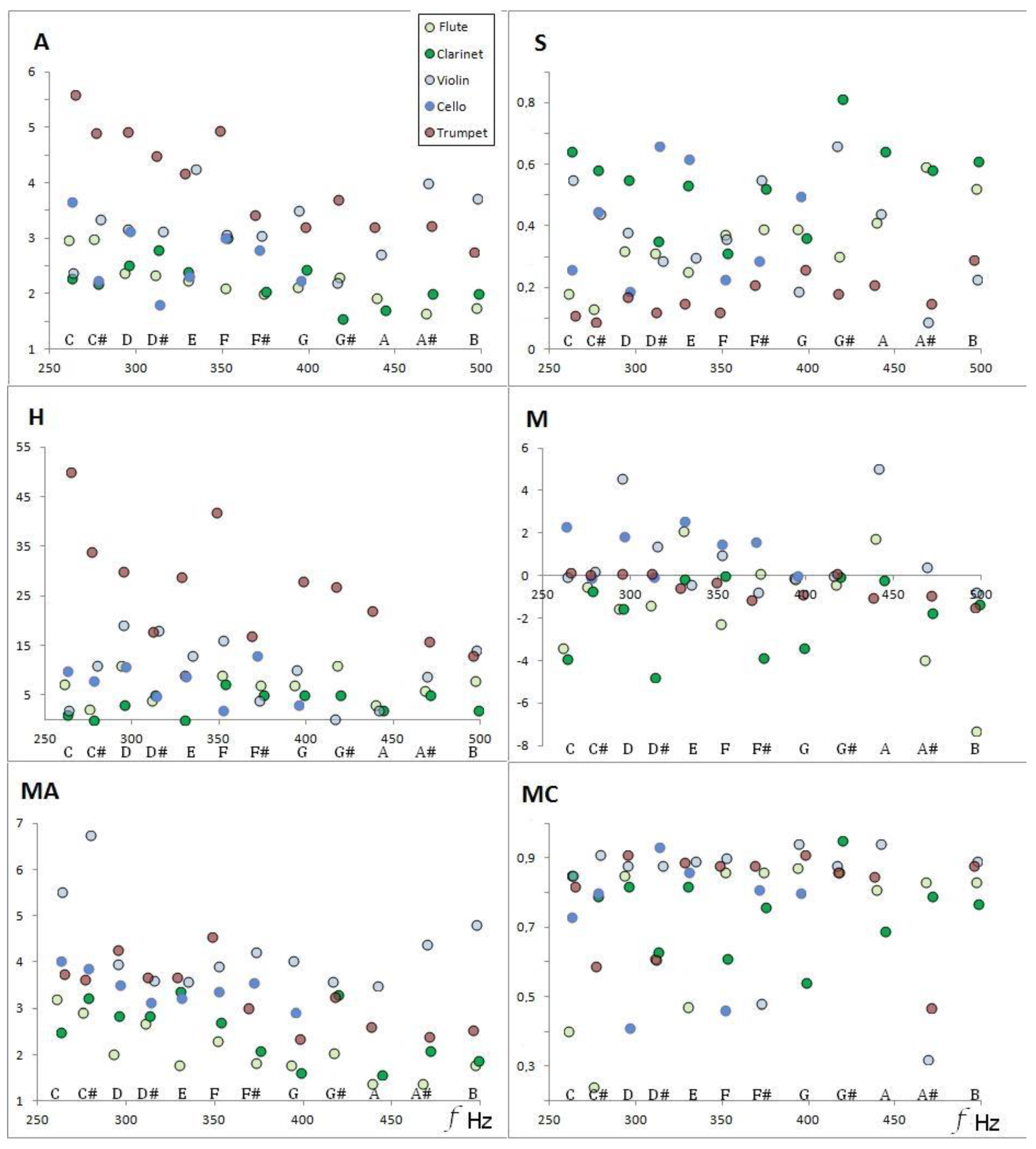
8]: “Affinity” A, “Sharpness” S, “Mean Affinity” MA, “Mean Contrast” MC, “Harmonicity” H, and “Monotony” M. The A and S timbral coefficients provide a measure of the frequency and relative amplitude of the fundamental signal with respect to the FFT spectrum. The coefficient H is a measure of the quantity and quality of the harmonics present in a spectral distribution. The coefficient M describes the average increase–decrease in the spectrum envelope. The MA and MC coefficients provide a measure of the mean frequency and mean amplitude of the spectral distribution, respectively (see
Table 1).
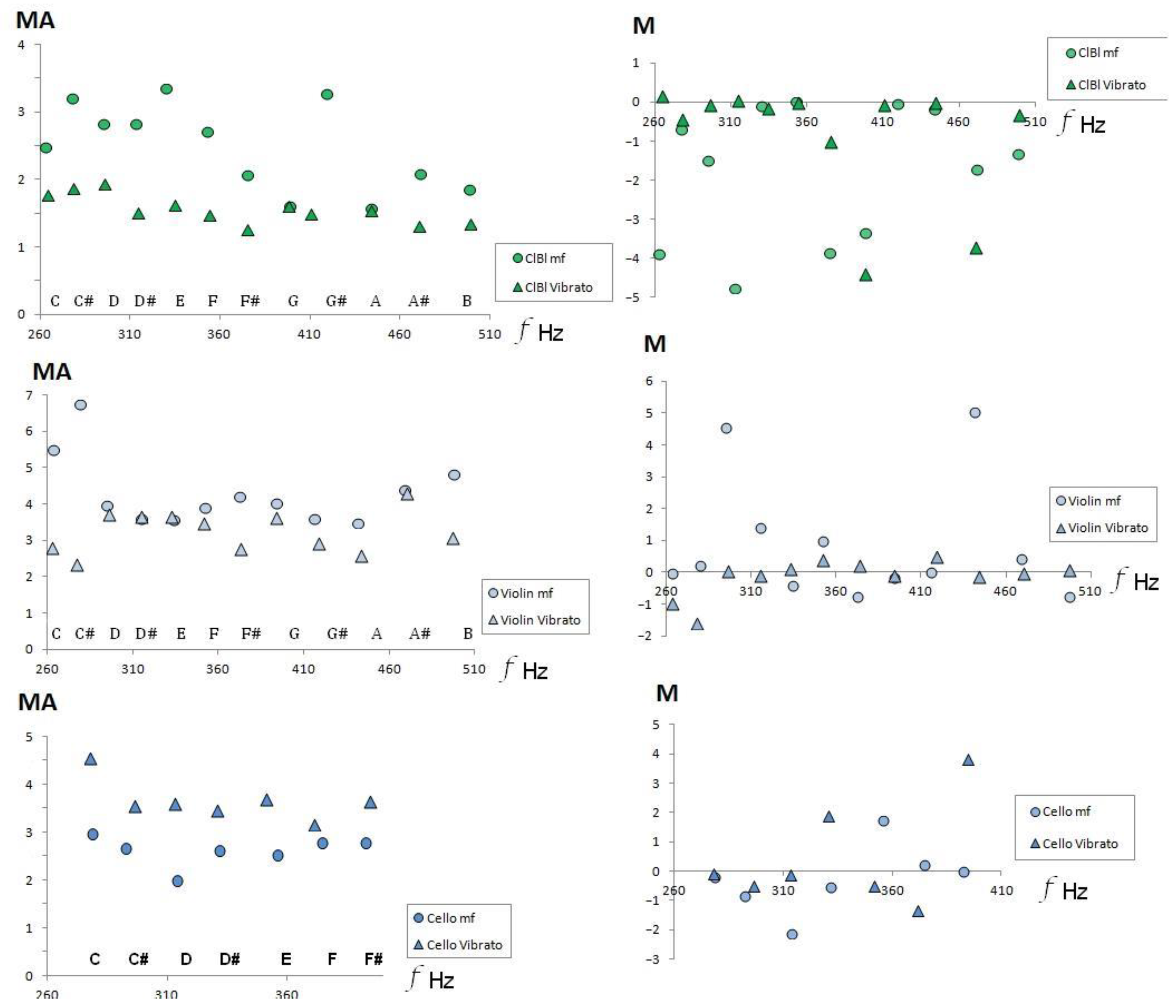
Figure 1 shows the timbral coefficients as a function of musical sounds and frequencies for the instruments selected from the Goodsound database, fourth octave, and mezzo-forte.
Then, each FFT spectrum can be represented by a mean 7-tuple (
f0,
A,
S,
H,
M,
MA,
MC) in an abstract configurational space. These 7-tuples that characterize the amplitude-frequency distribution present in each FFT spectrum provide a morphism between the frequency space and the seven-dimensional vector space. This 7-space can be called timbral space, since the musical timbre consists precisely of the set of spatial frequencies (formants and harmonics) that accompany each musical sound produced by a certain musical instrument, a certain dynamic, and the set of techniques of the performing musician. Note that the 7-tuples are real numbers and admit the definition of a module or Euclidean norm along with equivalence relations; therefore, they formally constitute a Moduli space, represented by a geometrical place that parametrizes the family of related algebraic objects [
11].
3. Euclidean Metric in Timbral Space
The timbral variations in the same musical sound due to the considered instrument (
Section 3.1), the musical dynamics (
Section 3.2), and the musical performance techniques used by the player, crescendo (
Section 3.3) and vibrato (
Section 3.4), are shown below through the Euclidean distance between the characteristic vectors of each FFT of the audio record, classified by musical sound (among the 12 possible in the fourth octave of the tempered scale).
All audio registers form a 7-tuple
,
A,
S,
H,
M,
MA,
MC) in abstract timbral space. So, any two audio records (subscripts
i and
j) can be timbrically compared via Euclidean distance as:
where ∆ represents the algebraic difference between timbral coefficients.
Although this distance is mainly governed by the difference in frequency values, it should be noted that, for the purposes of comparing musical timbres, it is assumed that the audios being compared have the same tone, that is, they correspond to the same musical sounds. Therefore, in practice, the difference in the fundamental frequencies of the real audios (first sum of the radical in Equation (1)) is small, of the order of tens. In general, it is evident that the timbral similarity cannot be provided only by the distance; the orientación with respect to the axes of the 7-dimensional space is also required. Its spatial location in the abstract space of seven dimensions is important. However, for sufficiently small distance values (i.e., fundamental frequencies very close) between the position of two audios in Timbral space, timbral proximity criteria can be established.
3.1. Instruments
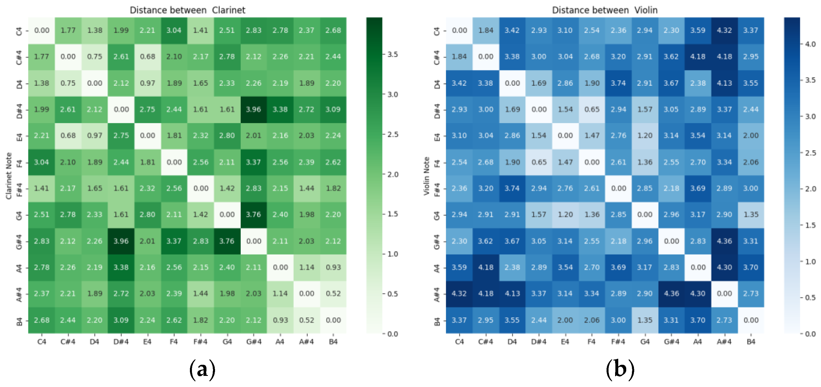
Figure 2 shows the standardized distances between monophonic audio recordings of instruments grouped by musical sounds. We observe that the registers are separated by notes, and the distance is a function of the tempered-scale sequence. The difference between the tables is due to the specific values of the timbral coefficients, as shown in
Figure 1. Each musical sound corresponding to an instrument occupies a single point of timbre space.
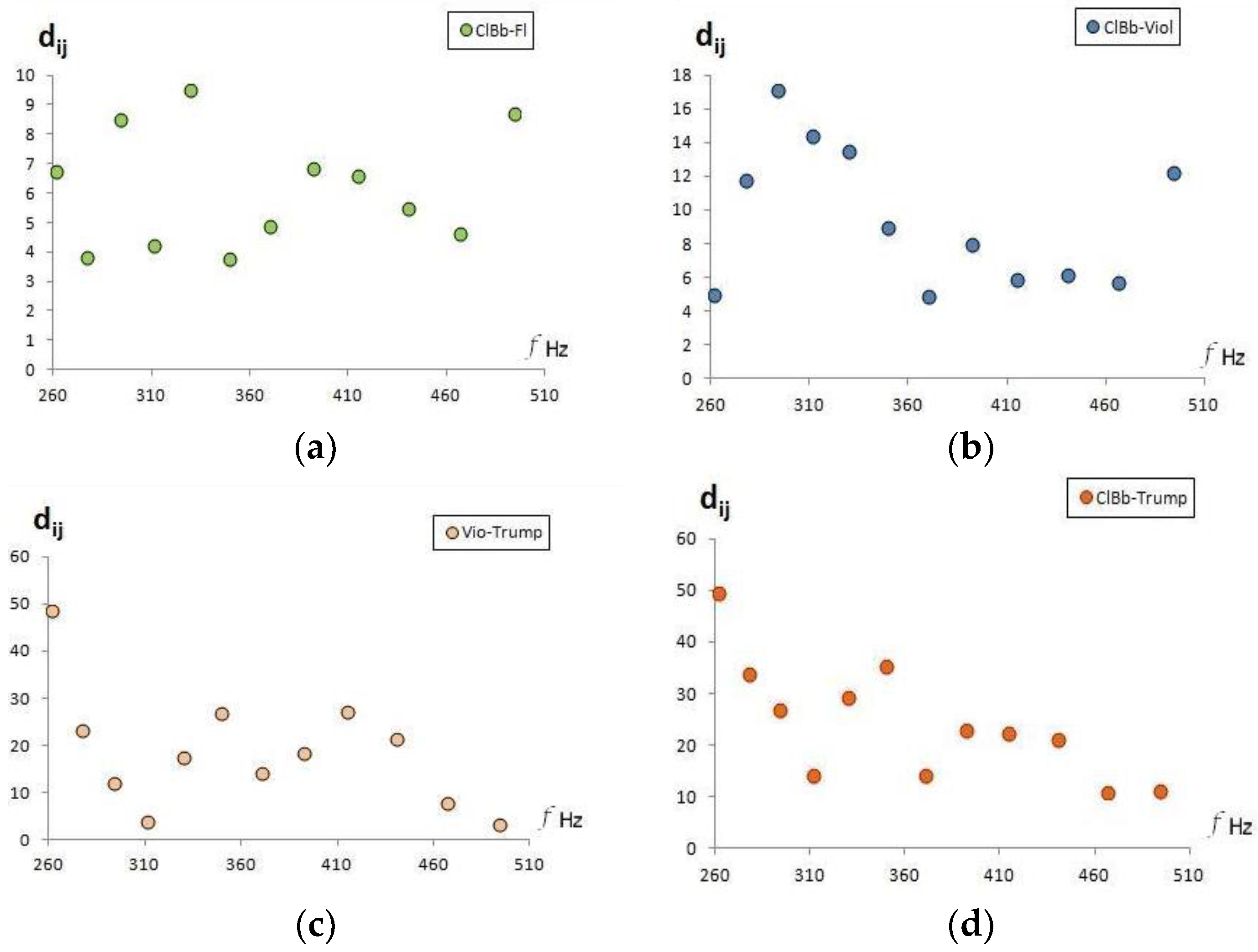
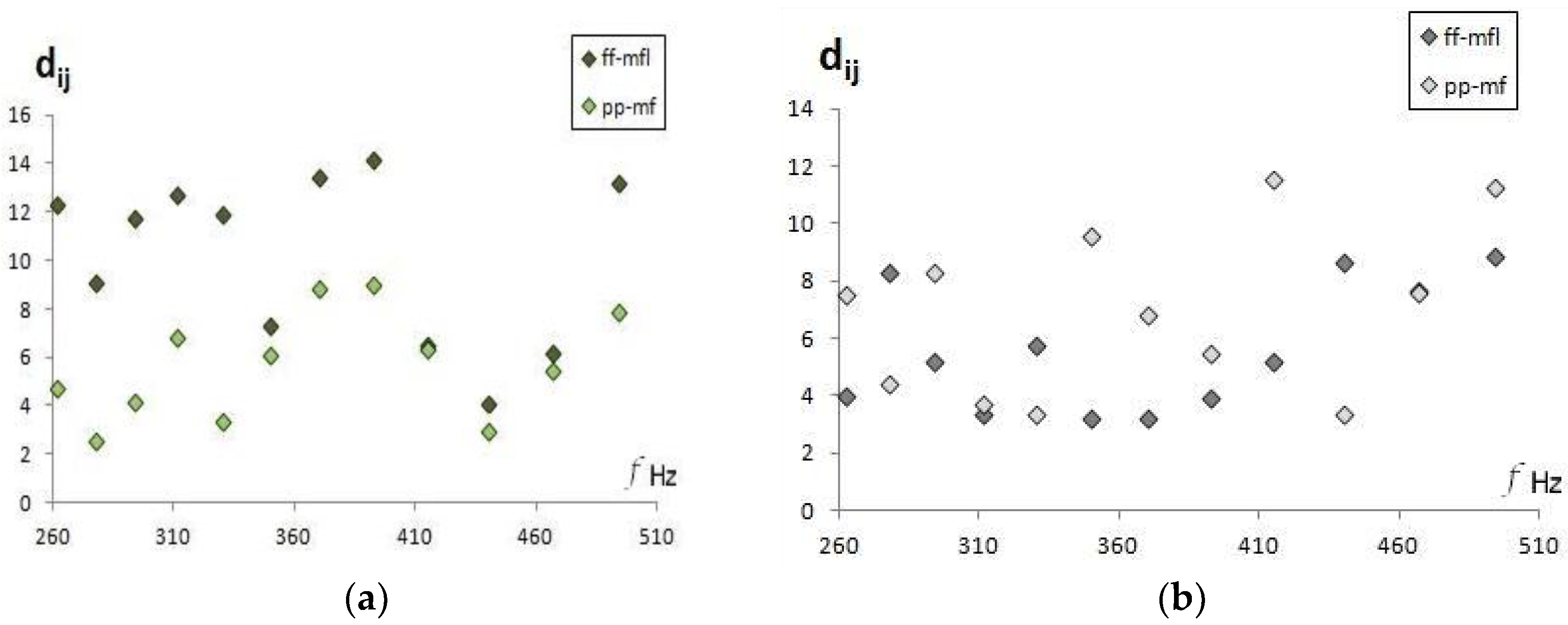
The distances between different instruments, grouped by musical sounds, are illustrated with various examples in
Figure 3. Note that for the same musical notes, the distances are smaller between instruments of the same type: flute and clarinet, both wooden aerophones (panel a). It is greater between aerophones and chordophones (panel b), between the chordophone and the wooden aerophone (panel c) and between the metal aerophone and the wooden aerophone (panel d).
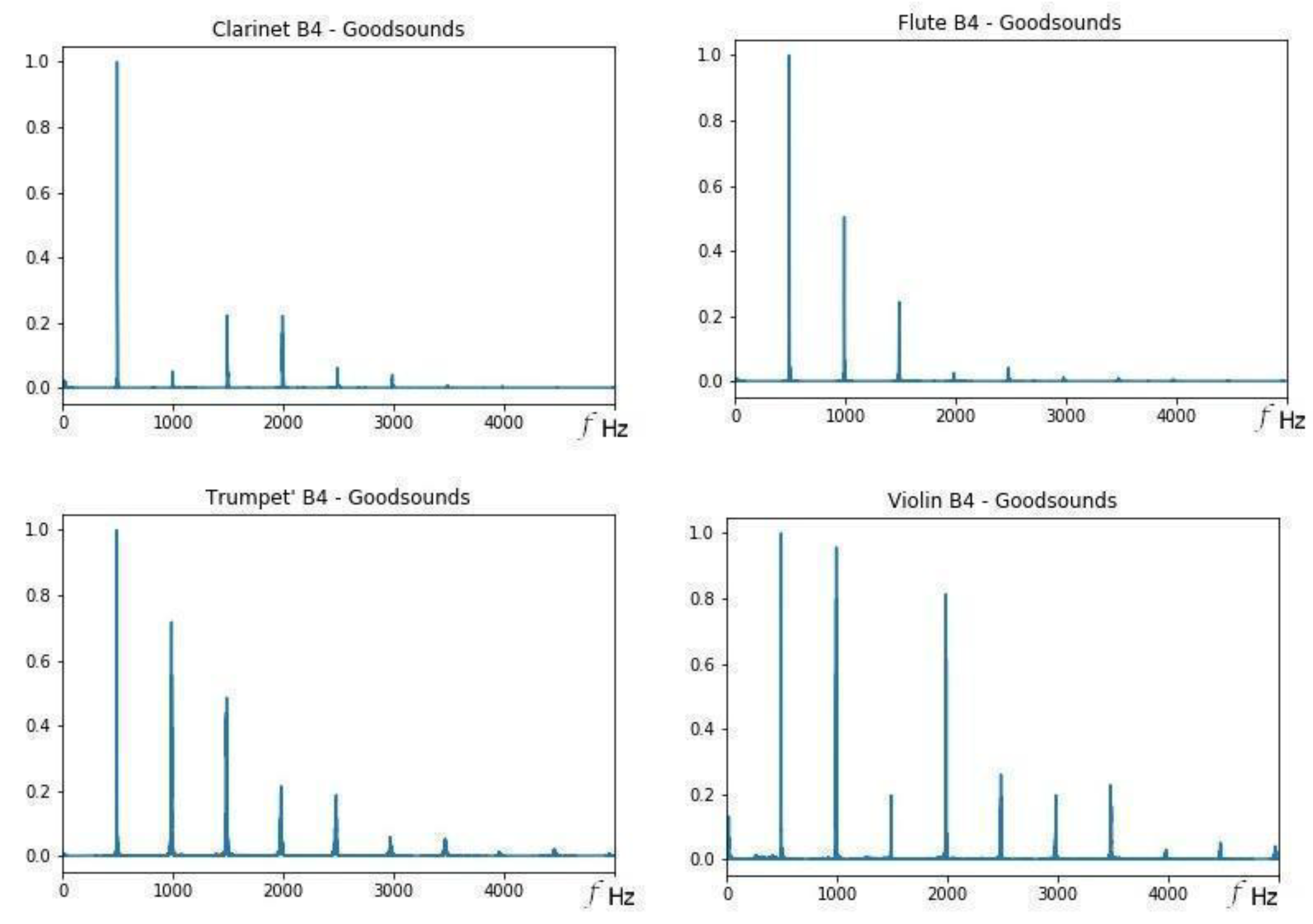
On the other hand, the results show that some sounds seem close to each other, although they were from different musical instruments with different classifications, for example, the B4 sound.
Figure 4 shows the FFTs for that sound. Notice the decrease in pulses, as well as the number and position of the partial frequencies. It cannot be affirmed that there is timbre similarity only because of the distance, since what defines the timbre is the vector and not only its module, and although the distance is equivalent between violin–trumpet and clarinet–trumpet, the sounds of these three instruments are in different regions of the timbre space (different clusters). To have timbral similarity, the sounds must be in the same cluster or region of the timbral space and must also be close to each other [
4]. This is equivalent to saying that they must be from audio recordings of the same instrument or type of instrument, and also have a distance that is less than the distance between adjacent musical sounds.
3.2. Musical Dynamics
Given a musical sound and an instrument, the variations in the intensity of the performance (musical dynamics) should produce timbrally similar sounds, and consequently, their timbral representation should be close to the mezzo-forte sound. Indeed, that is what is observed in
Figure 5 for the sounds in the Goodsound database compared to the Tinysol database records for different dynamics. Note that the minimum distances are always equal musical sounds and are less than 15.6, which is the minimum separation between two different musical notes of the tempered scale (between C4 and C#4), and therefore is also less than any other pair of sounds (in the fourth octave).
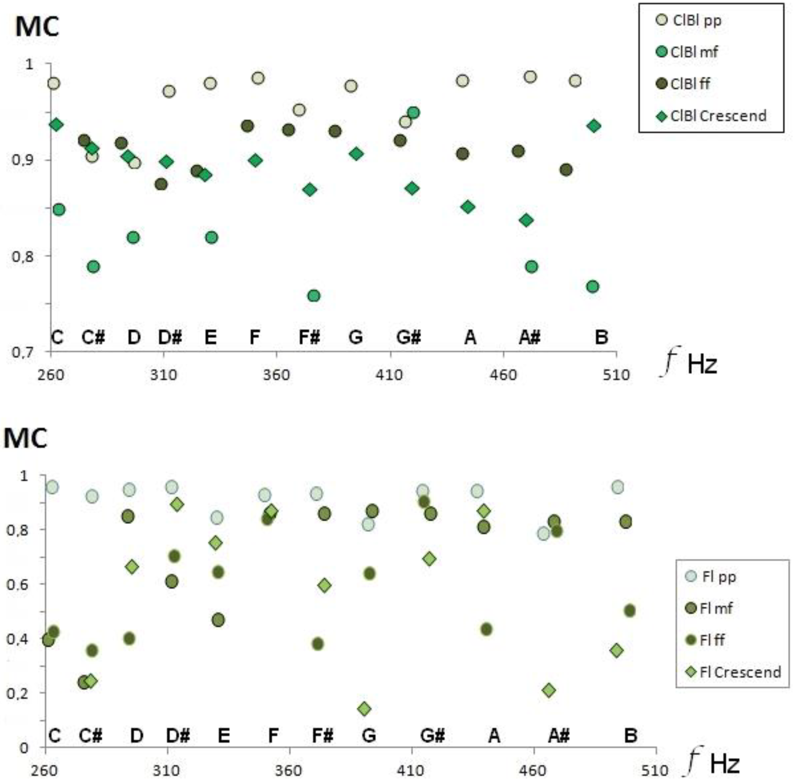
Timbral variations due to musical dynamics are shown by the increase in formants and harmonics in the FFT as we increase the intensity. Thus, the envelope of the FFT spectrum must be more extended, and the average value of the amplitudes changes. Hence, the acoustic descriptor of medium contrast, timbral coefficient MC, must vary in all musical sounds for the same instrument, as shown in
Figure 6 for clarinet and flute.
3.3. Crescendo
The crescendo is an instrumental performance technique that consists of the gradual variation in the musical dynamics. Consequently, the timbre effect with respect to timbre in the mezzo-forte audio recordings should be similar. For the flute and the clarinet, we can see in
Figure 6 how a decrease in the Mean Contrast (MC) occurs when we compare the dynamics of the pianissimo and mezzo-forte, also observing that the behavior of the crescendo effect decreases in the clarinet when we advance the frequencies.
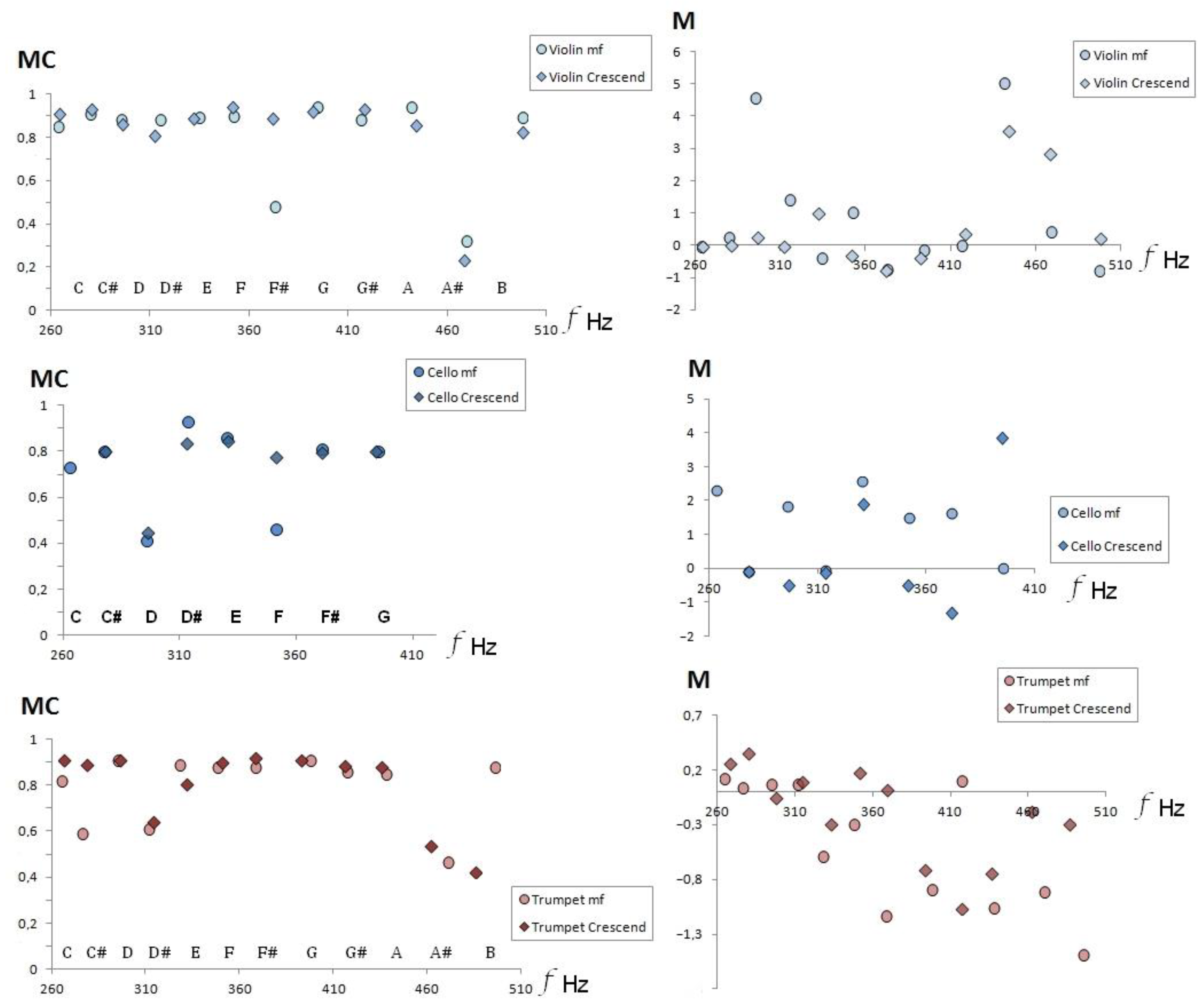
Figure 7 shows the same effect for the other instruments in the sample, so we can conjecture that, in general, the crescendo modifies the timbre coefficient of MC by incorporating more secondary frequencies in all instruments.
The right panel of
Figure 7 shows the values of the timbre coefficient M in the crescendo technique with respect to mezzo-forte audio recordings for both aerophones and chordophones. We notice that the timbral variation in the crescendo reduces the monotony value, which is a timbre coefficient that quantifies the envelope in the FFT. A decrease in the absolute value of monotony implies that the envelope softens, that is, that the average value of the variations in amplitude with respect to the fundamental frequency decreases.
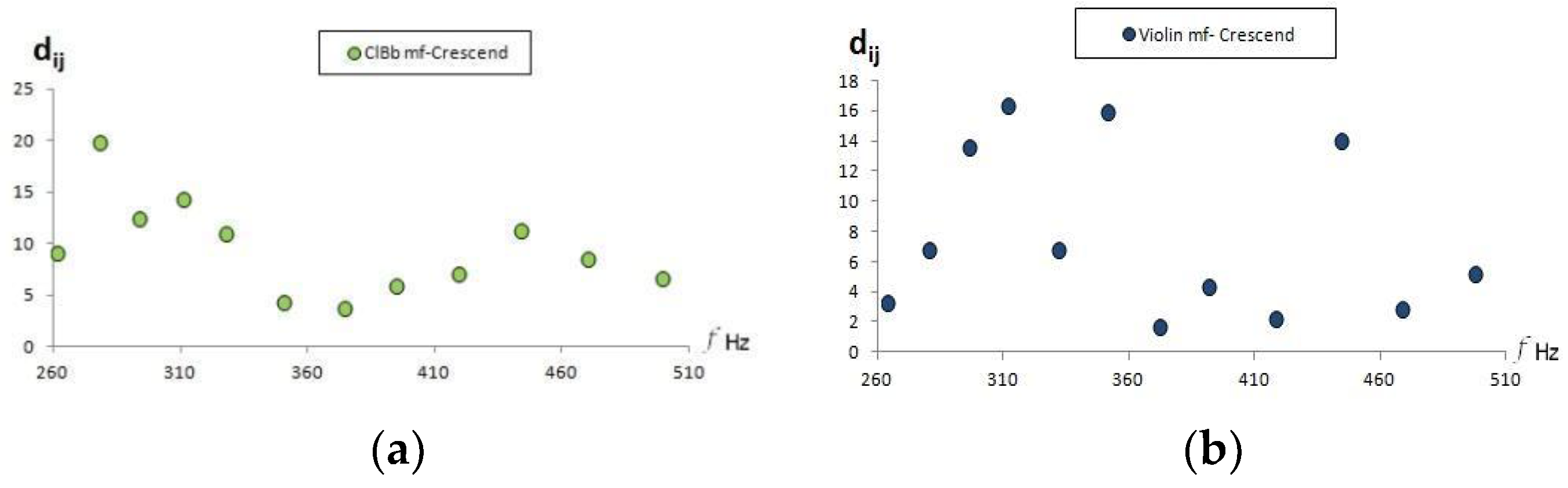
The audio recordings made with the crescendo technique must, similar to the dynamic musical variations, be close to the corresponding sounds in mezzo-forte. To illustrate this proximity, the Euclidean distances between each crescendo sound are shown in
Figure 8. Note again that all distances are less than 15.6 (separation between C4 and C#4 sounds).
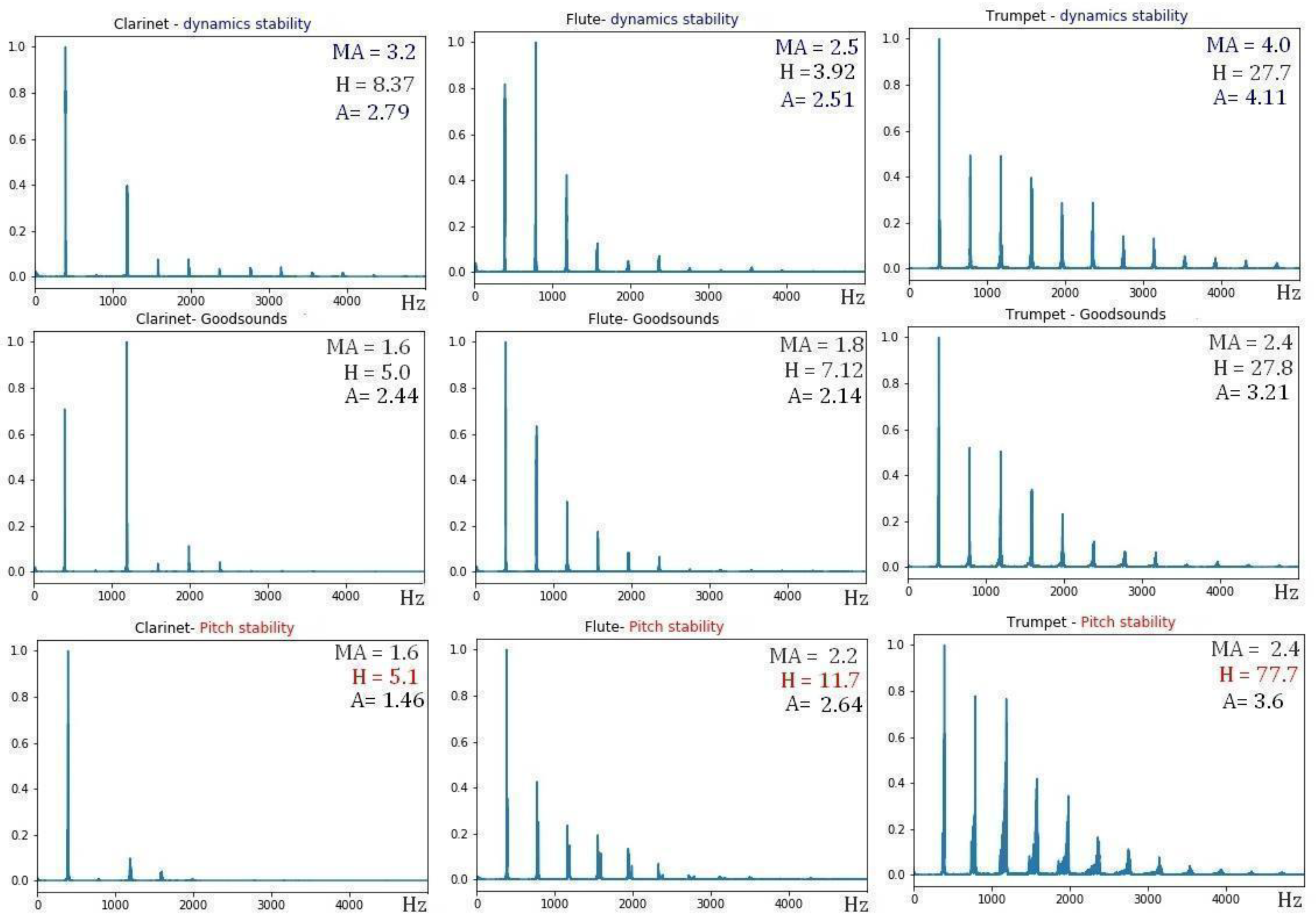
The crescendo technique increases the average intensity of the sounds; this implies that the formants and harmonics increase in intensity and, therefore, the value of the timbral coefficient of Affinity (A), Mean Affinity (MA), and Harmonicity (H) increases with respect to the values in mezzo-forte dynamics, as observed in the FFT of the audio recordings of
Figure 9 for the aerophones.
3.4. Vibrato
During vibrato, there is a slight variation in the fundamental frequency of the corresponding musical sound. Consequently, secondary frequencies that accompany the fundamental must appear; then, the Affinity (A) and Mean Affinity (MA) coefficients must change since they explicitly depend on the frequency values of the audio recording.
Figure 9 compares the Mean Affinity values with the Goodsound mezzo-forte records. Although the change in the value of MA is uniform with respect to the musical sounds of the fourth octave, it is not the same for all instruments. Vibrato increases the MA value on the cello and decreases it on the clarinet and violin. Similarly,
Figure 10 shows that vibrato also modifies monotony, as expected, because an increase in partial frequencies leads to a change in the envelope of the FFT spectrum.
The details of why some instruments increase the average of the partial frequencies (MA) and others decrease them are related to the geometry of the chordophone resonance box. The acoustics of chordophones are especially complicated because the wave generated by the vibration of the strings propagates in the air as a transversal wave, but in the sound-box, this pulsation originates transversal and longitudinal waves in the solid of the resonant cavity in addition to the transversal sound waves inside the air chamber. Therefore, it is beyond the objectives of this communication to elucidate this issue.
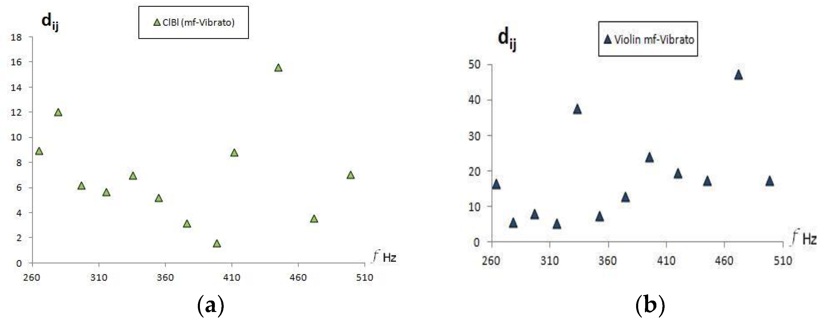
Also, since the variations in the frequency of the vibrato are less than the variation between adjacent musical notes in the tempered scale, it would be expected that the vibrato audio recordings would occur at relatively close distances to the Goodsounds mezzo-forte recordings.
Figure 11 shows a clarinet that behaves in the described manner, but in the case of the violin, greater distances appear in some sounds. This could be due to an incorrect musical performance of the vibrato or due to the effects of the violin sound box. Unlike the cello, the violin is more diverse in its musical performance of vibrato, due to the addition of the bow to the tension placed on the string by hand and due to the influence of the jaw resting on the body of the violin, which can modify the vibration modes of the formants.
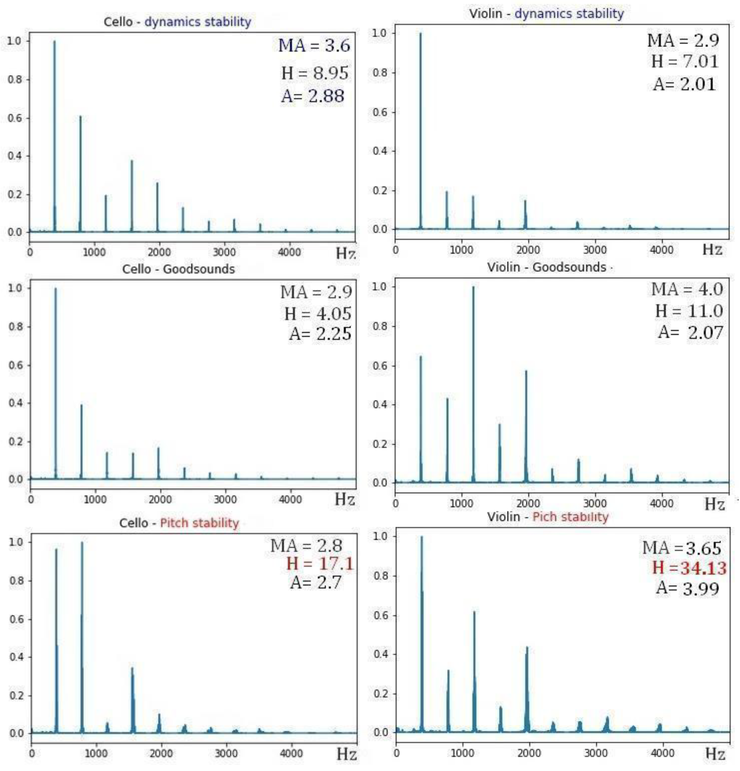
It is understandable that the oscillations in the main frequency in the vibrato increase the coefficient H since the partial frequencies that are generated will not be harmonic (greater H, less harmonicity), as can be seen in the lower panel of
Figure 9 and
Figure 12.
Figure 12 also shows that vibrato decreases the value of the Mean Affinity (MA) for chordophones.
In the upper panel of
Figure 12, it is observed that H does not always increase in the chordophones. This may be due to the interaction with the resonance box of the instrument, since the vibrations of some harmonics can cause destructive interference with the generated formants due to the geometry of the musical instrument being considered. However, the change due to musical dynamics is evidenced by the increase in Mean Affinity, even for chordophones. The variation in the Affinity is not conclusive, since, in this technique, as in vibrato, the musical performer can, according to their discretion and personal taste, modify the fundamental frequency during the performance of the crescendo; if they do this, the information will not be recorded in the Goodsound datasets.
Vibrato not only causes variations in frequency, but also oscillates the timbre of the sound, that is, causes the greater or lesser prevalence of one component or another. This oscillation in the sound quality caused by the vibrato violin is a characteristic feature of this instrument. The acoustic explanation of this feature of the violin lies in the properties of its sound box, which responds differently to very close frequency components. Finally, all instruments allow for the performer to make their own vibrato, and this resource is a very important part of characterizing the sound.
We have seen that the timbral coefficients allow for characterization of the timbral variations; however, it is worth asking how these acoustically motivated descriptors compare with other descriptors of the FFT based on statistical distributions. This is discussed in the next section.
4. Automatic Classification of Musical Timbres
The problems of classification can be resolved using supervised learning. These classification algorithms have been used in music style recognition problems through music feature extraction [
12], musical instrument classification problems [
13], and the use of an intelligent system for piano timbre recognition [
14], among other techniques. We are going to compare the classification capacities of the timbral coefficients proposed by González and Prati [
8] with some timbral features extracted using Librosa: Chroma stft, spectral contrast, spectral flatness, poly features, spectral centroid, spectral rolloff, and spectral bandwidth [
15].
For this, we use the TinySol database through the MIRDATA library [
16], which offers a standardization to work with audio attributes more efficiently. After defining the meta-attributes, we explore timbral classification capabilities by considering certain variations, such as instruments (violin, cello, transverse flute, clarinet, and trumpet), dynamics (pianissimo, mezzo-forte, and fortissimo), musical notes (considering the entire range of each instrument) and instrument families (chordophones, wooden aerophones, and metal aerophones).
We evaluated some classification algorithms, such as Random Forest (RF), Support Vector Classifier (SVC), K-Nearest Neighbor (KNN), and logistic regression, and we observed better statistical behavior in terms of classification for our subject of study with the Random Forest algorithm; this behavior occurs in benchmark tests [
17]. This is a conjoint learning method that combines multiple decision trees to create a more robust and accurate predictive model [
18].
We used the data split provided in the MIRDATA library, which divides the data into five folds. We applied a 5-fold cross-validation, where, in each iteration, one fold is used for testing and the remaining folds are used for training. The process is repeated five times, using a different test split each time. Using the Random Forest algorithm, we computed the mean accuracy using the timbral coefficients and the LibRosa features.
Table 2 presents the results.
To statistically compare the results, we use a paired T-test for each possible class. The last row of
Table 1 shows the
p-value of the test. Statistically significant differences were observed for the timbral coefficients when compared with Librosa in the classification by musical notes (pitch); this may be because the musical timbre, as an acoustic characteristic, is a frequency-independent property of the musical timbre. On the other hand, if we consider a significance interval of 99%, we can see that the timbral coefficients behave well when classifying instruments and families of instruments, and are better for the classification according to dynamics with respect to timbral features (Librosa).
5. Conclusions
Timbral variations in monophonic musical sounds can be characterized from an FFT analysis of audio recordings. More particularly, due to the techniques of musical performances of variations in amplitude (crescendo) and frequency (vibrato), these timbre variations differ between instruments according to their acoustic characteristics.
The acoustic FFT descriptors proposed by Gonzalez and Prati [
4,
8] provide a representation of the characteristic timbral space of each audio recording. Its position in the timbral space [
4] and the Euclidean distance between the registers allow for us to distinguish the timbral variations due to the family of instruments, the musical dynamics, and the variations in the execution technique. The latter can modify the envelope of the FFT and consequently change the values of monotonicity (M) and harmonicity (H). The crescendo modifies the Mean Contrast (MC) coefficient and the vibrato modifies the Affinity (A).
The Random Forest technique applied to evaluate the accuracy of the proposed classification shows statistically significant results for the FFT-Acoustic descriptors and timbral features of Librosa when classifying instruments, dynamics, and families of instruments, observing a better classification by pitch in the FFT-Acoustic descriptors when comparing them with Librosa features. It is important to perceive that Librosa does not discriminate between the dynamic variations in crescendo and vibrato, while the FFT-Acoustic descriptors do allow for them to be discriminated.
Author Contributions
Conceptualization, Y.G. and R.C.P.; methodology, Y.G. and R.C.P.; software, Y.G. and R.C.P.; validation, Y.G. and R.C.P.; formal analysis, Y.G. and R.C.P.; investigation, Y.G. and R.C.P.; resources, Y.G. and R.C.P.; data curation, Y.G. and R.C.P.; writing—original draft preparation, Y.G.; writing—review and editing, Y.G. and R.C.P.; visualization, Y.G.; supervision, R.C.P.; project administration, Y.G. and R.C.P.; funding acquisition, Y.G. and R.C.P. All authors have read and agreed to the published version of the manuscript.
Funding
This study was financed in part by the Coordenação de Aperfeiçoamento de Pessoal de nível Superior—Brasil (CAPES)—Finance Code 001.
Institutional Review Board Statement
Not applicable.
Informed Consent Statement
Not applicable.
Data Availability Statement
Conflicts of Interest
The authors declare no conflict of interest.
References
- Randel, D.M. The Harvard Dictionary of Music; Harvard University Press: Cambridge, MA, USA, 2003; p. 224. [Google Scholar]
- Gough, C. Musical acoustics. In Springer Handbook of Acoustics; Springer: New York, NY, USA, 2014; pp. 567–701. [Google Scholar]
- Almeida, A.; Schubert, E.; Wolfe, J. Timbre Vibrato Perception and Description. Music Percept. 2021, 38, 282–292. [Google Scholar] [CrossRef]
- Gonzalez, Y.; Prati, R.C. Similarity of musical timbres using FFT-acoustic descriptor analysis and machine learning. Eng 2023, 4, 555–568. [Google Scholar] [CrossRef]
- Gonzalez, Y.; Prati, R. Acoustic Analysis of Musical Timbre of Wooden Aerophones. Rom. J. Acoust. Vib. 2023, 19, 134–142. [Google Scholar]
- McAdams, S. The perceptual representation of timbre. In Timbre: Acoustics, Perception, and Cognition; Springer: Cham, Switzerland, 2019; pp. 23–57. [Google Scholar]
- Peeters, G.; Giordano, B.L.; Susini, P.; Misdariis, N.; McAdams, S. The timbre toolbox: Extracting audio descriptors from musical signals. JASA J. Acoust. Soc. Am. 2011, 130, 2902–2916. [Google Scholar] [CrossRef] [PubMed]
- Gonzalez, Y.; Prati, R.C. Acoustic descriptors for characterization of musical timbre using the Fast Fourier Transform. Electronics 2022, 11, 1405. [Google Scholar] [CrossRef]
- Romaní Picas, O.; Parra-Rodriguez, H.; Dabiri, D.; Tokuda, H.; Hariya, W.; Oishi, K.; Serra, X. A real-time system for measuring sound goodness in instrumental sounds. In Proceedings of the 138th Audio Engineering Society Convention, AES 2015, Warsaw, Poland, 7–10 May 2015; pp. 1106–1111. [Google Scholar]
- Carmine, E.; Ghisi, D.; Lostanlen, V.; Lévy, F.; Fineberg, J.; Maresz, Y. TinySOL: An Audio Dataset of Isolated Musical Notes. Zenodo 2020. Available online: https://zenodo.org/record/3632193#.Y-QrSnbMLIU (accessed on 15 May 2022).
- Kollár, J. Moduli of varieties of general type. In Handbook of Moduli; Vol. II, 131–157, Adv. Lect. Math.(ALM); Int. Press: Somerville, MA, USA, 2013; p. 25. [Google Scholar]
- Zhang, K. Music style classification algorithm based on music feature extraction and deep neural network. Wirel. Commun. Mob. Comput. 2021, 2021, 9298654. [Google Scholar] [CrossRef]
- Chakraborty, S.S.; Parekh, R. Improved musical instrument classification using cepstral coefficients and neural networks. In Methodologies and Application Issues of Contemporary Computing Framework; Springer: Singapore, 2018; pp. 123–138. [Google Scholar]
- Lu, Y.; Chu, C. A Novel Piano Arrangement Timbre Intelligent Recognition System Using Multilabel Classification Technology and KNN Algorithm. Comput. Intell. Neurosci. 2022, 2022, 2205936. [Google Scholar] [CrossRef] [PubMed]
- McFee, B.; Raffel, C.; Liang, D.; Ellis, D.P.; McVicar, M.; Battenberg, E.; Nieto, O. librosa: Audio and music signal analysis in python. In Proceedings of the 14th python in science conference 2015, Austin, TX, USA, 6–12 July 2015; pp. 18–25. [Google Scholar]
- Bittner, R.M.; Fuentes, M.; Rubinstein, D.; Jansson, A.; Choi, K.; Kell, T. Mirdata: Software for Reproducible Usage of Datasets. In Proceedings of the 20th International Society for Music Information Retrieval (ISMIR) Conference, Delft, The Netherlands, 4–8 November 2019. [Google Scholar]
- Fernández-Delgado, M.; Cernadas, E.; Barro, S.; Amorim, D. Do we need hundreds of classifiers to solve real world classification problems? J. Mach. Learn. Res. 2014, 15, 3133–3181. [Google Scholar]
- Michalski, R.S.; Carbonell, J.G.; Mitchell, T.M. Machine Learning: An Artificial Intelligence Approach; Springer: Berlin/Heidelberg, Germany, 2013. [Google Scholar]
Figure 1.
Representations in the frequency of the FFT–acoustic descriptors (timbral coefficients) for the Goodsound dataset.
Figure 1.
Representations in the frequency of the FFT–acoustic descriptors (timbral coefficients) for the Goodsound dataset.
Figure 2.
Matrix of Euclidean distances (statistically normalized by converting each value into its typical score) between musical sounds of the clusters that make up the proper subspace of each musical instrument: (a) Clarinet (b) Violin (c) Flute and (d) Trumpet.
Figure 2.
Matrix of Euclidean distances (statistically normalized by converting each value into its typical score) between musical sounds of the clusters that make up the proper subspace of each musical instrument: (a) Clarinet (b) Violin (c) Flute and (d) Trumpet.
Figure 3.
Comparison of Euclidean distances between musical sounds of different instruments: (a) clarinet–flute; (b) clarinet–violin; (c) violin–trumpet; (d) clarinet–trumpet.
Figure 3.
Comparison of Euclidean distances between musical sounds of different instruments: (a) clarinet–flute; (b) clarinet–violin; (c) violin–trumpet; (d) clarinet–trumpet.
Figure 4.
Fourier Transforms of the B4 Goodsound for different instruments. See the text for details.
Figure 4.
Fourier Transforms of the B4 Goodsound for different instruments. See the text for details.
Figure 5.
Euclidean distances between musical sounds from mezzo-forte Goodsounds and their cluster dynamics using the Tynisol dataset with the proper subspace of each musical instrument: (a) clarinet; (b) flute.
Figure 5.
Euclidean distances between musical sounds from mezzo-forte Goodsounds and their cluster dynamics using the Tynisol dataset with the proper subspace of each musical instrument: (a) clarinet; (b) flute.
Figure 6.
Variations in the MC timbre coefficient as a function of musical dynamics: clarinet, upper panel and flute, lower panel. Also, note the variation in M when performing the crescendo technique (
Section 3.3).
Figure 6.
Variations in the MC timbre coefficient as a function of musical dynamics: clarinet, upper panel and flute, lower panel. Also, note the variation in M when performing the crescendo technique (
Section 3.3).
Figure 7.
Medium contrast (left panel) and monotony (right panel) timbral coefficients, in the Goodsound database audios of violin (top), cello (center) and trumpet (bottom).
Figure 7.
Medium contrast (left panel) and monotony (right panel) timbral coefficients, in the Goodsound database audios of violin (top), cello (center) and trumpet (bottom).
Figure 8.
Euclidean distances between the musical sounds of the crescendo and mezzo-forte Goodsound audio records: (a) clarinet; (b) violin.
Figure 8.
Euclidean distances between the musical sounds of the crescendo and mezzo-forte Goodsound audio records: (a) clarinet; (b) violin.
Figure 9.
FFTs G4 sound of clarinet (Left Column), flute (Central Column) and trumpet (Right Column); normal register mezzo-forte (middle row), with crescendo technique (upper row) and vibrato (lower row). The values of the timbral coefficients of the Mean Affinity (MA), Harmonicity (H), and Affinity (A) are highlighted.
Figure 10.
Medium Affinity (left panel) and monotony (right panel) timbral coefficients, in the Goodsound database audios of clarinet (top), violin (center), and cello (bottom).
Figure 10.
Medium Affinity (left panel) and monotony (right panel) timbral coefficients, in the Goodsound database audios of clarinet (top), violin (center), and cello (bottom).
Figure 11.
Euclidean distances between the musical sounds of the vibrato and mezzo-forte Goodsound audio recordings: (a) clarinet; (b) violin.
Figure 11.
Euclidean distances between the musical sounds of the vibrato and mezzo-forte Goodsound audio recordings: (a) clarinet; (b) violin.
Figure 12.
FFTs of G4 sound: cello (left column) and violin (right column); normal register mezzo-forte (middle row), with crescendo technique (upper row) and vibrato (lower row). The values of the timbral coefficients of Mean Affinity (MA), Harmonicity (H), and Affinity (A) are highlighted.
Figure 12.
FFTs of G4 sound: cello (left column) and violin (right column); normal register mezzo-forte (middle row), with crescendo technique (upper row) and vibrato (lower row). The values of the timbral coefficients of Mean Affinity (MA), Harmonicity (H), and Affinity (A) are highlighted.
Table 1.
Timbral coefficients associated with the FFT of monophonic musical sounds.
Table 1.
Timbral coefficients associated with the FFT of monophonic musical sounds.
| Coefficient | Operational Definition | Description |
|---|
| (A) Affinity | | Relative measurement of the centroid with respect to the fundamental frequency |
| (S) Sharpness | | Relative measure of the amplitude of the fundamental frequency |
| (MA) Medium affinity | | Average deviation of the partial frequencies from the average frequency |
| (MC) Medium Contrast | | Mean deviation of the partial amplitudes from the amplitude of the fundamental frequency |
| (H) Harmonicity | | Average value of the harmony of the partial frequencies |
| (M) Monotony | | Deviation from regularity in the distribution of amplitudes with respect to frequencies |
Table 2.
Comparative results of the Random Forest classification algorithm (mean accuracy ± Standard Deviation) for category recognition: musical instrument, musical dynamics, musical note, and musical instrument families.
Table 2.
Comparative results of the Random Forest classification algorithm (mean accuracy ± Standard Deviation) for category recognition: musical instrument, musical dynamics, musical note, and musical instrument families.
| Instrument | Dynamics | Pitch | Family |
|---|
| Timbral Coefficients [8] | 0.78 ± 0.02 | 0.63 ± 0.038 | 0.65 ± 0.046 | 0.92 ± 0.017 |
| Timbral features (Librosa) | 0.89 ± 0.029 | 0.97 ± 0.011 | 0.22 ± 0.014 | 0.91 ± 0.018 |
| Test T (p-value) | 0.0000209 | 0.0000136 | 0.000115 | 0.0185 |
| Disclaimer/Publisher’s Note: The statements, opinions and data contained in all publications are solely those of the individual author(s) and contributor(s) and not of MDPI and/or the editor(s). MDPI and/or the editor(s) disclaim responsibility for any injury to people or property resulting from any ideas, methods, instructions or products referred to in the content. |
© 2023 by the authors. Licensee MDPI, Basel, Switzerland. This article is an open access article distributed under the terms and conditions of the Creative Commons Attribution (CC BY) license (https://creativecommons.org/licenses/by/4.0/).


