
Assessment of Techniques for Detection of Transient Radio-Frequency Interference (RFI) Signals: A Case Study of a Transient in Radar Test Data

Abstract
:1. Introduction
1.1. Investigation Overview
1.2. Overview of State-of-the-Art
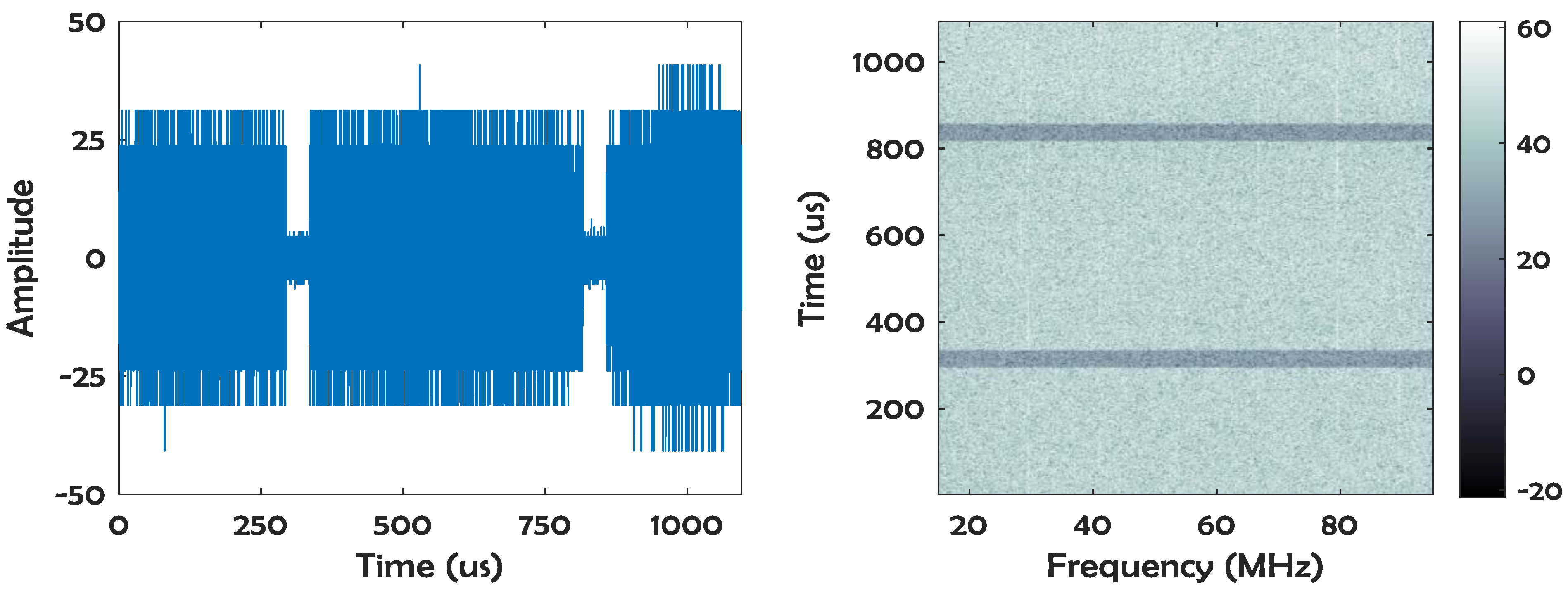
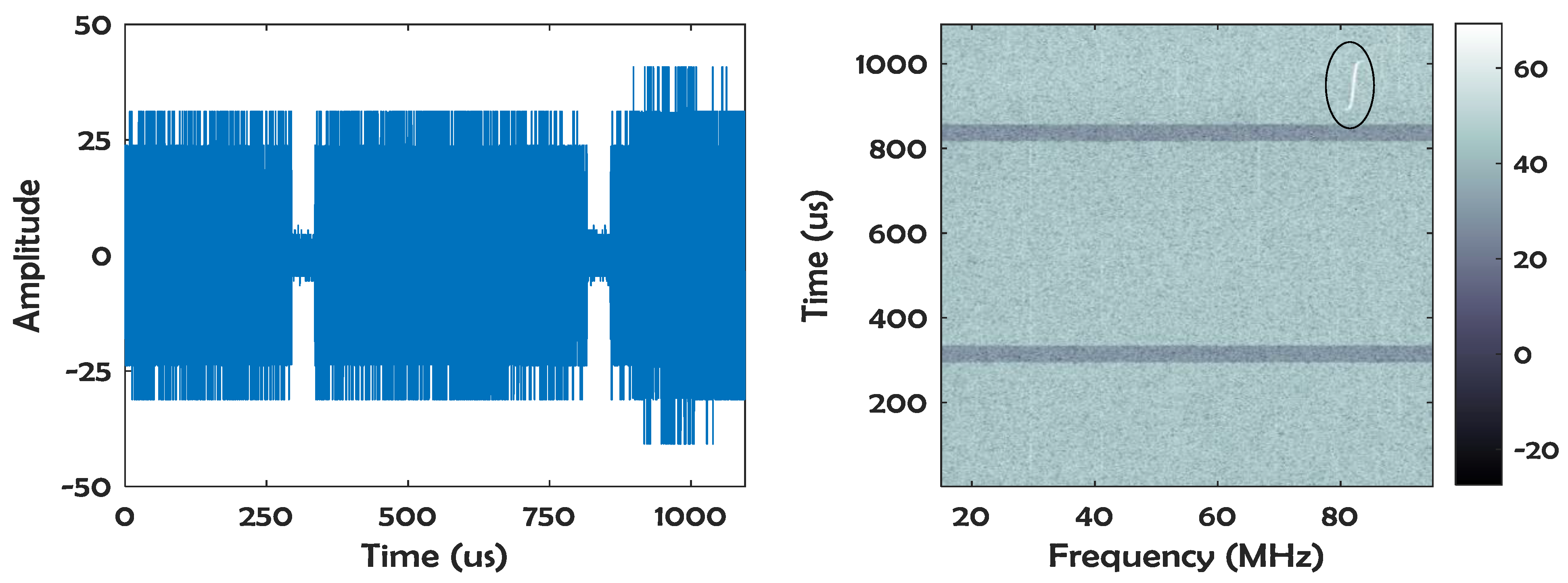
2. Data
3. Data Analysis Methodology
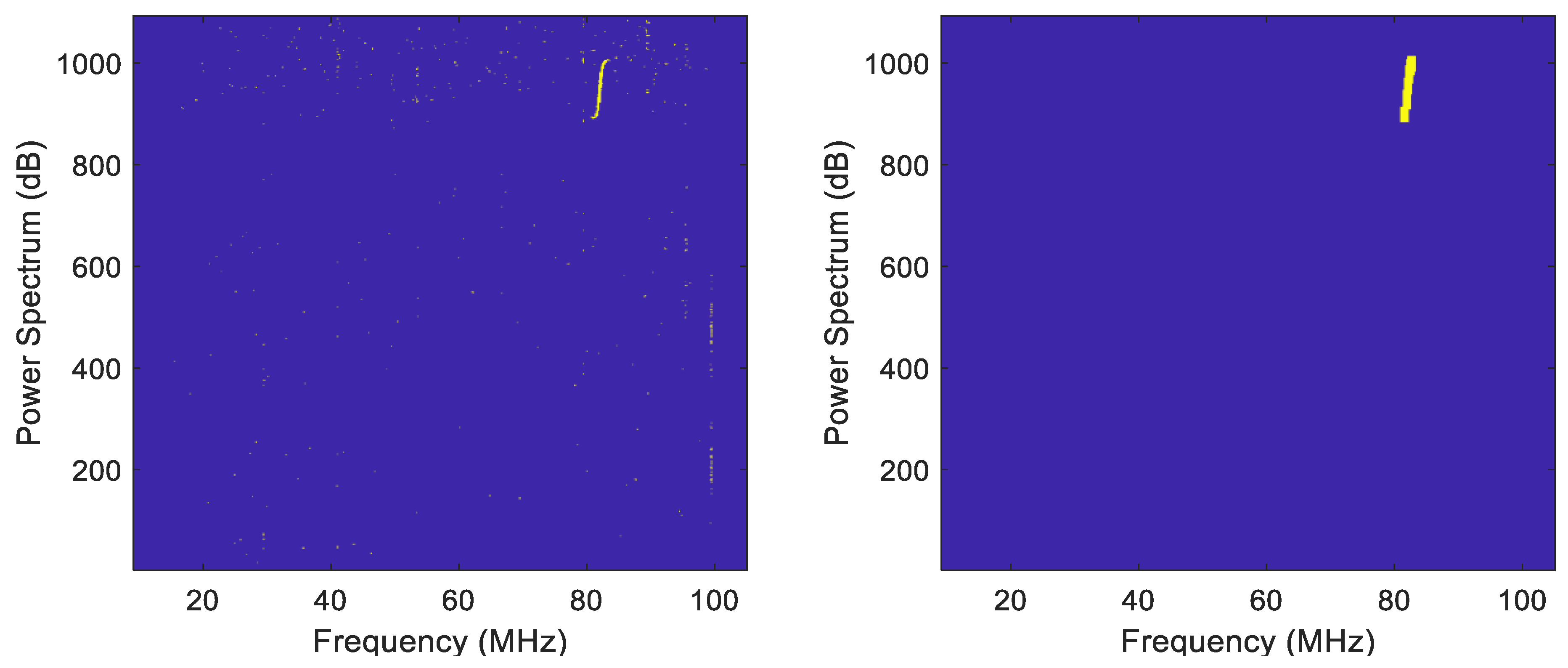
3.1. Computer Vision
3.2. Convolutional Neural Network
3.3. Statistical Decision Theory
4. Results
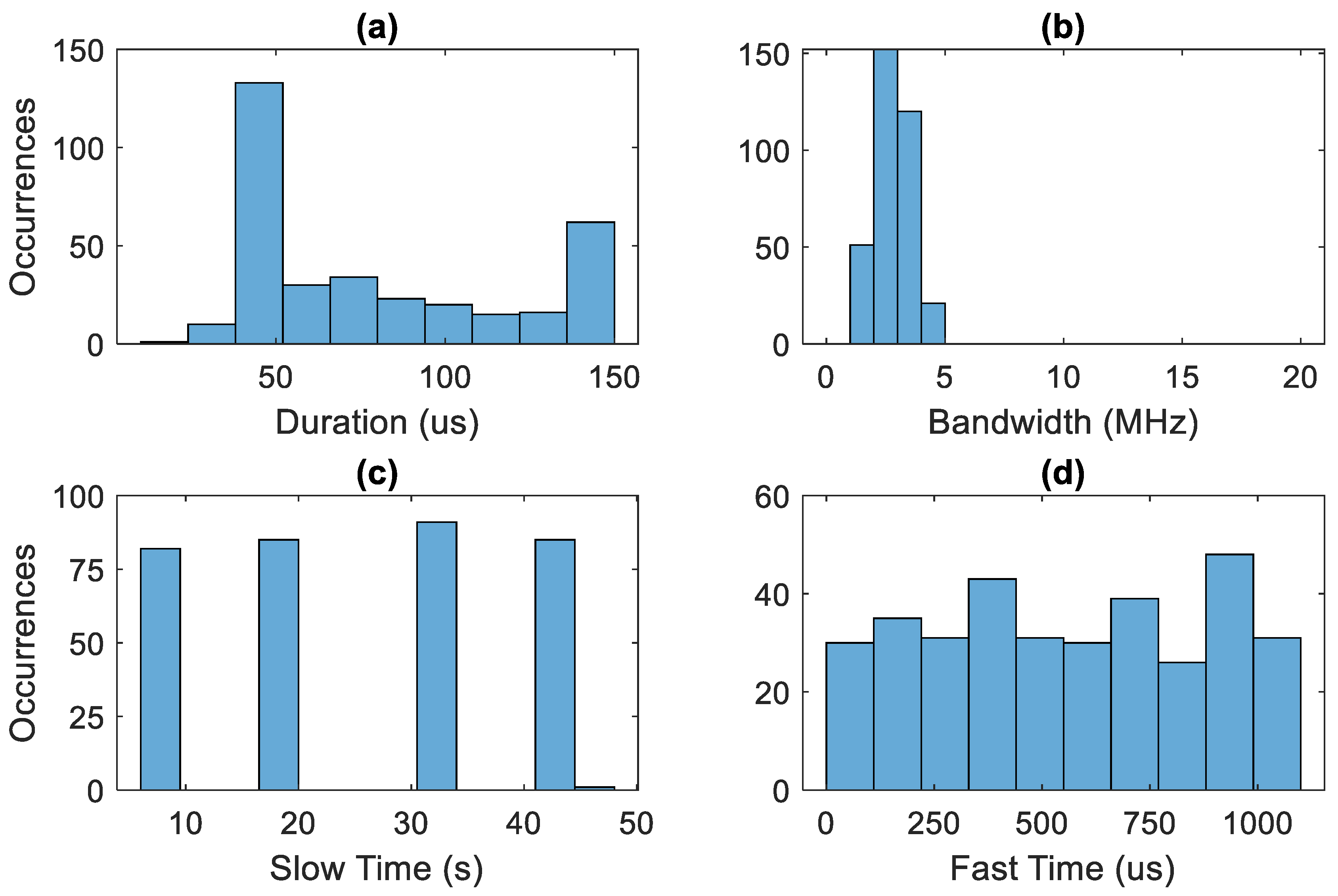
4.1. Generation of Training and Validation Data
4.2. CVA Results
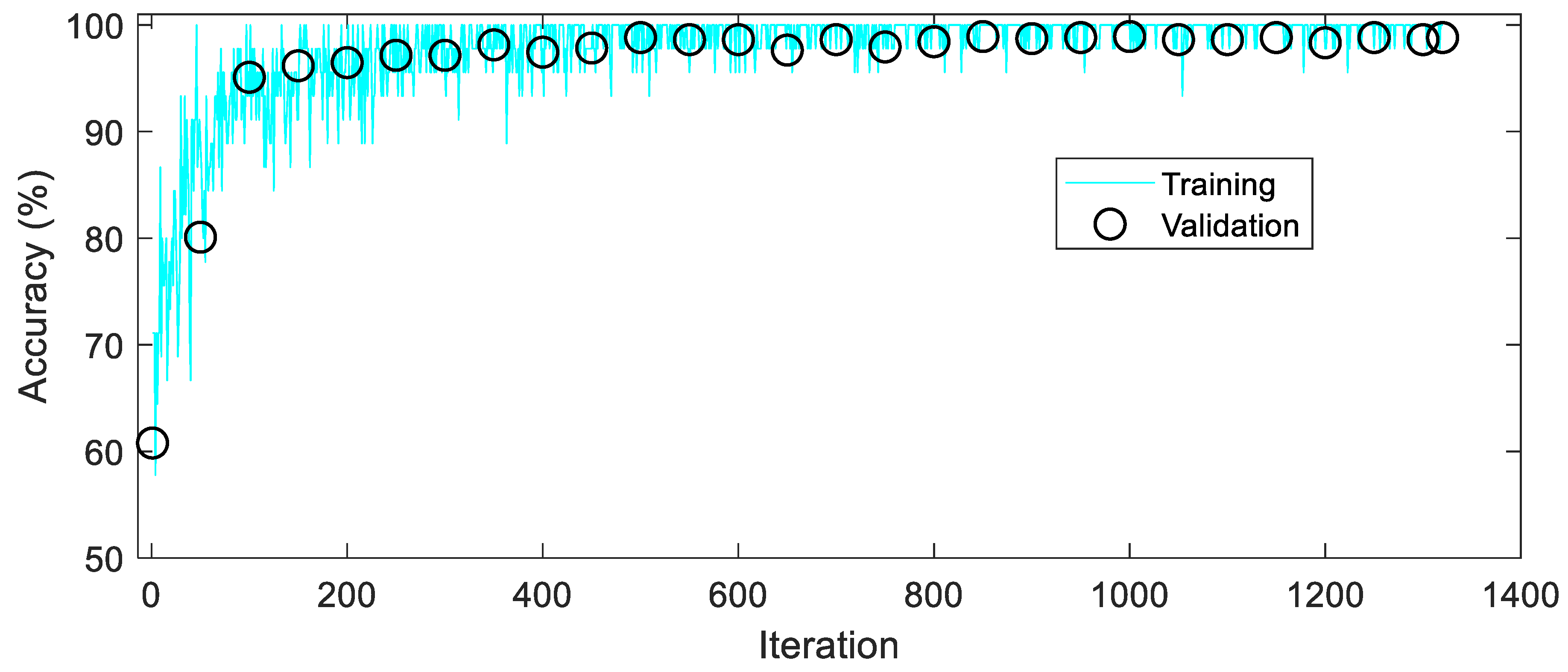
4.3. CNN Results
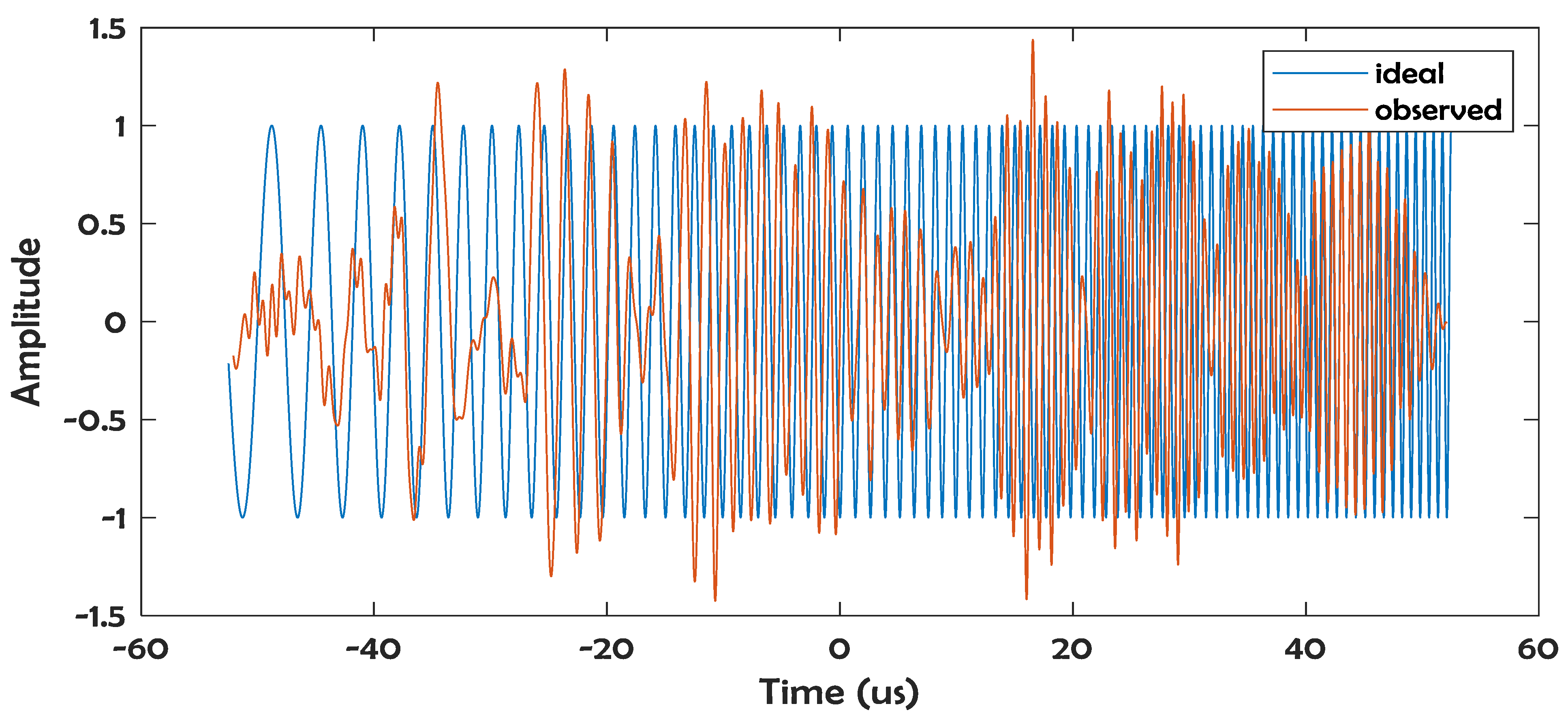
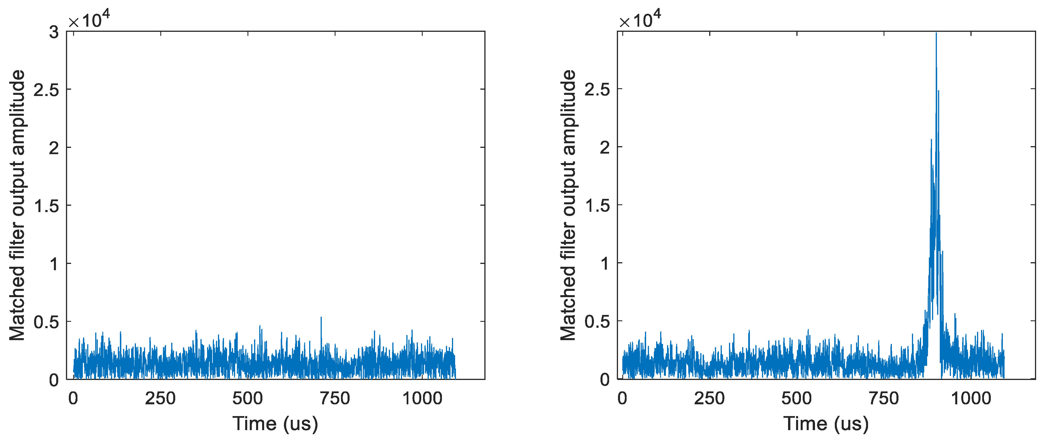
4.4. MF Results
5. Conclusions
Author Contributions
Funding
Institutional Review Board Statement
Informed Consent Statement
Data Availability Statement
Acknowledgments
Conflicts of Interest
Appendix A
References
- Zhou, H.; Wen, B.; Wu, S. Dense radio frequency interference suppression in HF radars. IEEE Signal Process. Lett. 2005, 12, 361–364. [Google Scholar] [CrossRef]
- Misra, S.; Kristensen, S.S.; Sobjaerg, S.S.; Skou, N. CoSMOS: Performance of kurtosis algorithm for radio frequency interference detection and mitigation. In Proceedings of the IGARSS, Barcelona, Spain, 23–28 July 2007; pp. 2714–2717. [Google Scholar]
- Leshem, A.; van der Veen, A.-J.; Deprettere, E. Detection and blanking of GSM interference in radio-astronomical observations. In Proceedings of the 2nd IEEE Workshop on Signal Processing Advances in Wireless Communications, Annapolis, MD, USA, 9–12 May 1999; pp. 374–377. [Google Scholar]
- Yang, D.; Xiao, D.; Zhang, L. The parameters estimation and the feature extraction of underwater transient signal. In Proceedings of the IEEE International Conference on Signal Processing, Communications and Computing (ICSPCC), Xi’an, China, 14–16 September 2011; pp. 1–4. [Google Scholar]
- Soltanieh, N.; Norouzi, Y.; Yang, Y.; Chandra Karmakar, N. A review of radio frequency fingerprinting techniques. IEEE J. Radio Freq. Identif. 2020, 4, 222–233. [Google Scholar] [CrossRef]
- Medaiyese, O.O.; Ezuma, M.; Lauf, A.P.; Adeniran, A.A. Hierarchical learning framework for UAV detection and identification. IEEE J. Radio Freq. Identif. 2022, 6, 176–188. [Google Scholar] [CrossRef]
- Van Trees, H.L. Detection, Estimation, and Modulation Theory Part I: Detection, Estimation, and Linear Modulation Theory; Wiley: New York, NY, USA, 2001. [Google Scholar]
- Friedlander, B.; Porat, B. Performance analysis of transient detectors based on a class of linear data transforms. IEEE Trans. Inf. Theory 1992, 38, 665–673. [Google Scholar] [CrossRef]
- Guepie, B.K.; Fillatre, L.; Nikiforov, I. Detecting a Suddenly Arriving Dynamic Profile of Finite Duration. IEEE Trans. Inf. Theory 2017, 63, 3039–3052. [Google Scholar] [CrossRef]
- Besson, O.; Coluccia, A.; Chaumette, E.; Ricci, G.; Vincent, F. Generalized likelihood ratio test for detection of Gaussian rank-one signals in Gaussian noise with unknown statistics. IEEE Trans. Signal Process. 2017, 65, 1082–1092. [Google Scholar] [CrossRef]
- Besson, O. Adaptive detection of Gaussian rank-one signals using adaptively whitened data and Rao, gradient and Durbin tests. IEEE Signal Process. Lett. 2023, 30, 399–402. [Google Scholar] [CrossRef]
- Yang, J.; Gu, H.; Hu, C.; Zhang, X.; Gui, G.; Gacanin, H. Deep complex-valued convolutional neural network for drone recognition based on RF fingerprinting. Drones 2022, 6, 374. [Google Scholar] [CrossRef]
- Itschner, S.; Li, X. Radio frequency interference (RFI) detection in instrumentation radar systems: A deep learning approach. In Proceedings of the IEEE Radar Conference, Boston, MA, USA, 22–26 April 2019; pp. 1–5. [Google Scholar]
- Jiang, M.; Cui, B.; Yu, Y.-F.; Cao, Z. DM-Free curvelet based denoising for astronomical single pulse detection. IEEE Access 2019, 7, 107389–107399. [Google Scholar] [CrossRef]
- Czech, D.; Mishra, A.; Inggs, M. A CNN and LSTM-based approach to classifying transient radio frequency interference. Astron. Comput. 2018, 25, 52–57. [Google Scholar] [CrossRef]
- Agarwal, D.; Aggarwal, K.; Burke-Spolaor, S.; Lorimer, D.R.; Garver-Daniels, N. FETCH: A deep-learning based classifier for fast transient classification. MNRAS 2020, 497, 1661–1674. [Google Scholar] [CrossRef]
- Shapiro, L.G.; Stockman, G.C. Computer Vision; Prentice-Hall: Englewood Cliffs, NJ, USA, 2001. [Google Scholar]
- Davies, E.R. Machine Vision: Theory, Algorithms, Practicalities; Morgan-Kaufmann: Amsterdam, The Netherlands, 2005. [Google Scholar]
- Zhao, J.; Masood, R.; Seneviratne, S. A review of computer vision methods in network security. IEEE Commun. Surv. Tutor. 2021, 23, 1838–1878. [Google Scholar] [CrossRef]
- MathWorks. Matlab Image Processing Toolbox User’s Guide; The Mathworks: Natick, MA, USA, 2022. [Google Scholar]
- Khan, S.; Rahmani, H.; Shah, S.A.A.; Bennamoun, M. A Guide to Convolutional Neural Networks for Computer Vision; Springer: Cham, Switzerland, 2018. [Google Scholar]
- Ujan, S.; Navidi, N.; Landry, R., Jr. An efficient radio frequency interference (RFI) recognition and characterization using end-to-end transfer learning. Appl. Sci. 2020, 10, 6885. [Google Scholar] [CrossRef]
- Beale, M.H.; Hagan, M.T.; Demuth, H.B. Matlab Deep Learning Toolbox User’s Guide; The Mathworks: Natick, MA, USA, 2022. [Google Scholar]
- Garth, L.M.; Poor, H.V. Detection of non-Gaussian signals: A paradigm for modern statistical signal processing. Proc. IEEE 1994, 82, 1061–1095. [Google Scholar] [CrossRef]
- Kailath, T.; Poor, H.V. Detection of stochastic processes. IEEE Trans. Inf. Theory 1998, 44, 2230–2259. [Google Scholar] [CrossRef]
- Abraham, D.A. Underwater Acoustic Signal Processing; Springer: Cham, Switzerland, 2019. [Google Scholar]
- Abatzoglou, T.J. Fast maximum likelihood joint estimation of frequency and frequency rate. IEEE Trans. Aerosp. Electron. Syst. 1986, AES-22, 708–715. [Google Scholar] [CrossRef]
- Boyer, R.; Abed-Meraim, K. Damped and delayed sinusoidal model for transient signals. IEEE Trans. Signal Process. 2005, 53, 1720–1730. [Google Scholar] [CrossRef]
- Golden, S.; Friedlander, B. Maximum likelihood estimation, analysis, and applications of exponential polynomial signals. IEEE Trans. Signal Process. 1999, 47, 1493–1501. [Google Scholar] [CrossRef]


| Method | Est. Run Time (s) | Validation Data | Correct |
|---|---|---|---|
| Computer Vision Algorithm (CVA) | 40 | 1020 spectrograms | 1016 |
| Convolutional Neural Net (CNN) | 45 | 1020 spectrograms | 1007 |
| Matched filter (MF) | 25 | 1020 range lines | 990 |
Disclaimer/Publisher’s Note: The statements, opinions and data contained in all publications are solely those of the individual author(s) and contributor(s) and not of MDPI and/or the editor(s). MDPI and/or the editor(s) disclaim responsibility for any injury to people or property resulting from any ideas, methods, instructions or products referred to in the content. |
© 2023 by the California Institute of Technology. Government sponsorship acknowledged. Licensee MDPI, Basel, Switzerland. This article is an open access article distributed under the terms and conditions of the Creative Commons Attribution (CC BY) license (https://creativecommons.org/licenses/by/4.0/).
Share and Cite
Durden, S.L.; Vilnrotter, V.A.; Shaffer, S.J. Assessment of Techniques for Detection of Transient Radio-Frequency Interference (RFI) Signals: A Case Study of a Transient in Radar Test Data. Eng 2023, 4, 2191-2203. https://doi.org/10.3390/eng4030126
Durden SL, Vilnrotter VA, Shaffer SJ. Assessment of Techniques for Detection of Transient Radio-Frequency Interference (RFI) Signals: A Case Study of a Transient in Radar Test Data. Eng. 2023; 4(3):2191-2203. https://doi.org/10.3390/eng4030126
Chicago/Turabian StyleDurden, Stephen L., Victor A. Vilnrotter, and Scott J. Shaffer. 2023. "Assessment of Techniques for Detection of Transient Radio-Frequency Interference (RFI) Signals: A Case Study of a Transient in Radar Test Data" Eng 4, no. 3: 2191-2203. https://doi.org/10.3390/eng4030126