
Toward More Realistic Social Distancing Policies via Advanced Feedback Control


Abstract
:1. Introduction
- takes only a finite number of numerical values,
- remains constant during some time interval, two weeks here, in our computer simulations.
2. SIR and Open-Loop Control
2.1. Flatness
2.2. Elementary Formulae for Open-Loop Control
- ,
- contrarily to [18] we do not start with ,
3. Closed-Loop Control
- , ,
- the constant parameter , which does not need to be precisely determined, is chosen such that the three terms in Equation (11) are of the same magnitude.
- subsumes the poorly known internal structure and the external disturbances.
- An estimate of is given [56] by the integralwhich in practice may be computed via a digital filter.
4. Computer Simulations
4.1. Unrealistic Scenarios
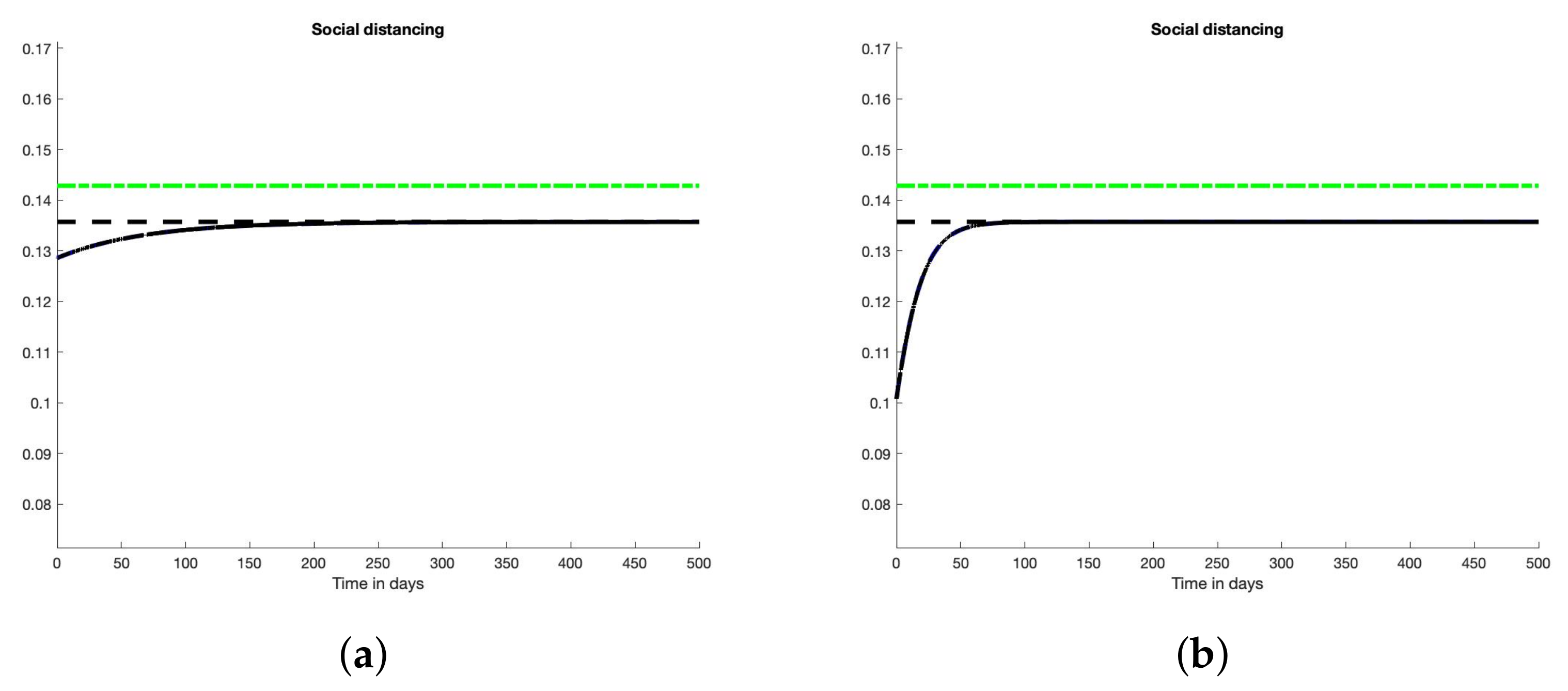
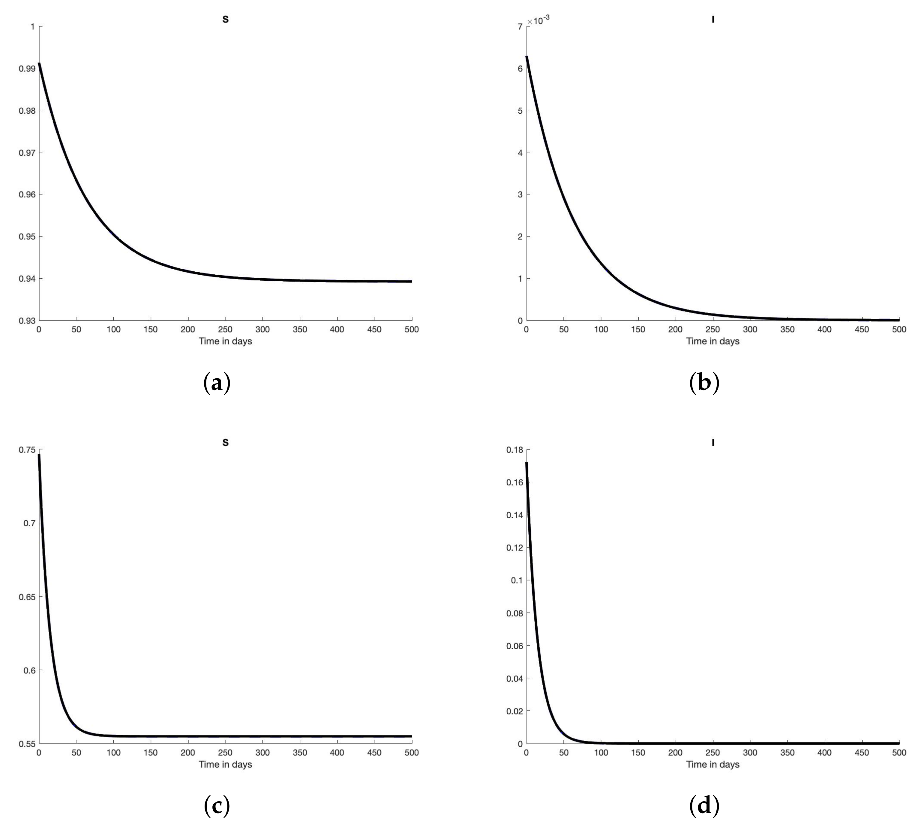
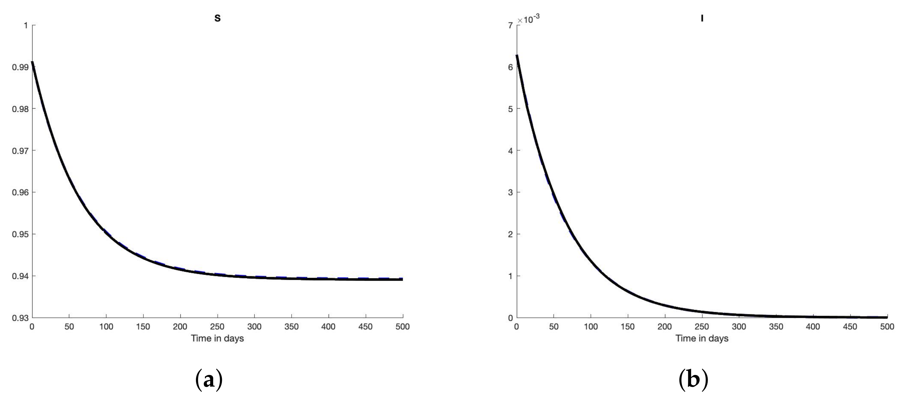
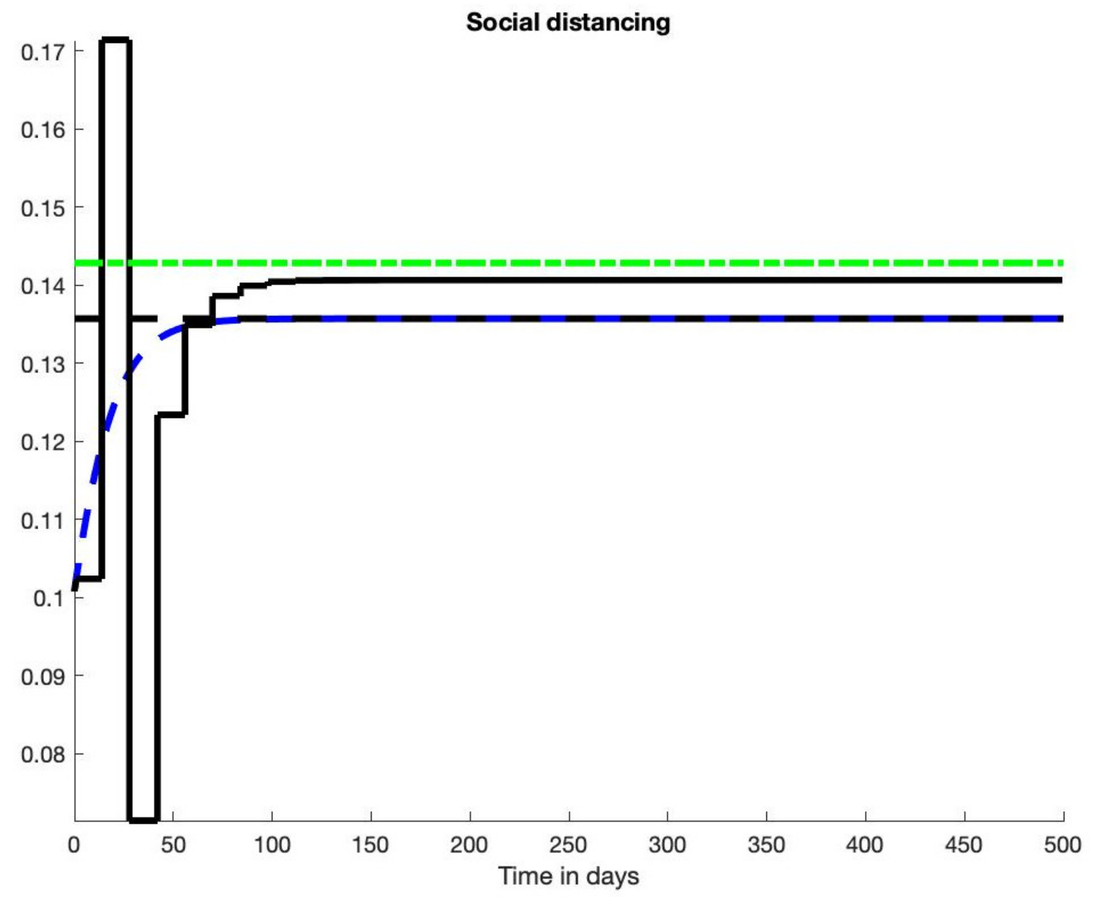
4.1.1. Scenario 1
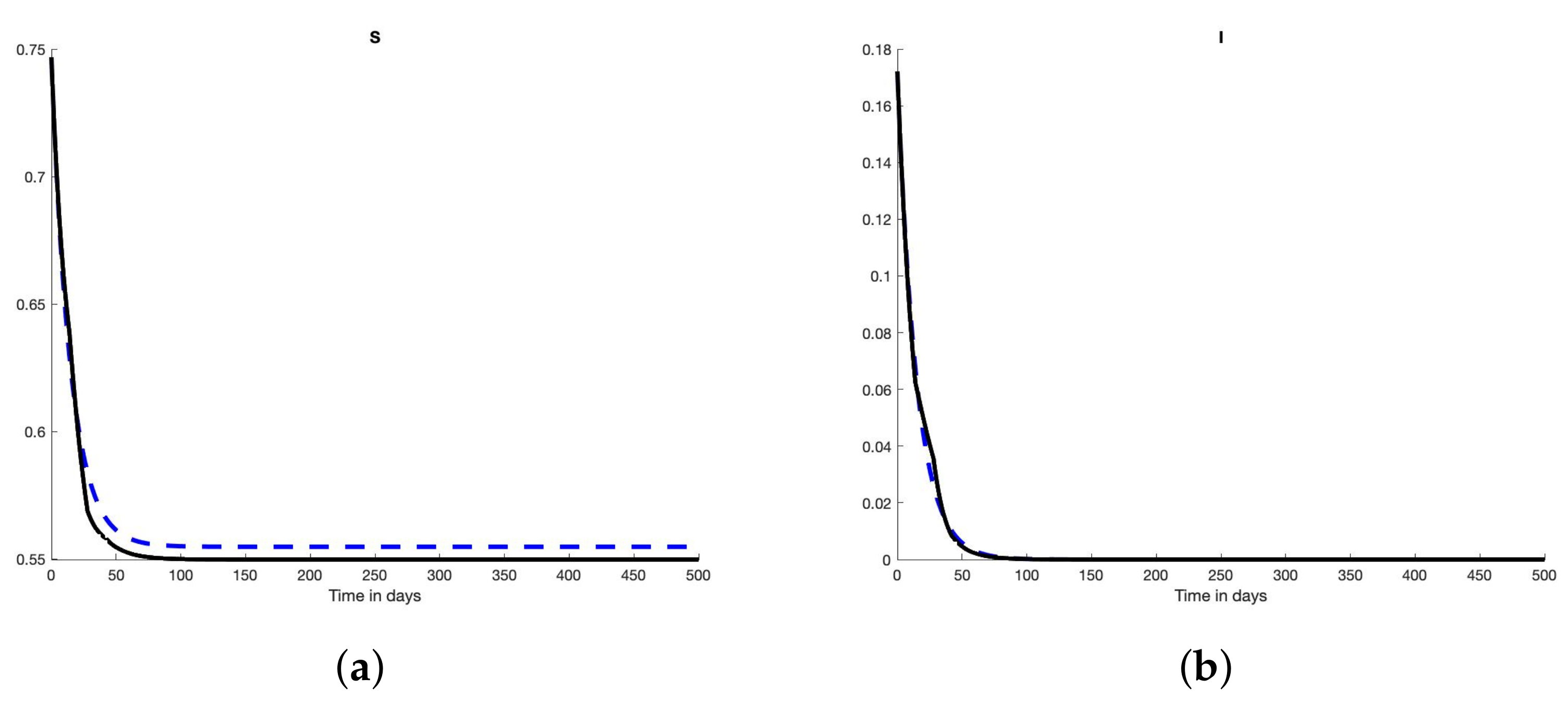
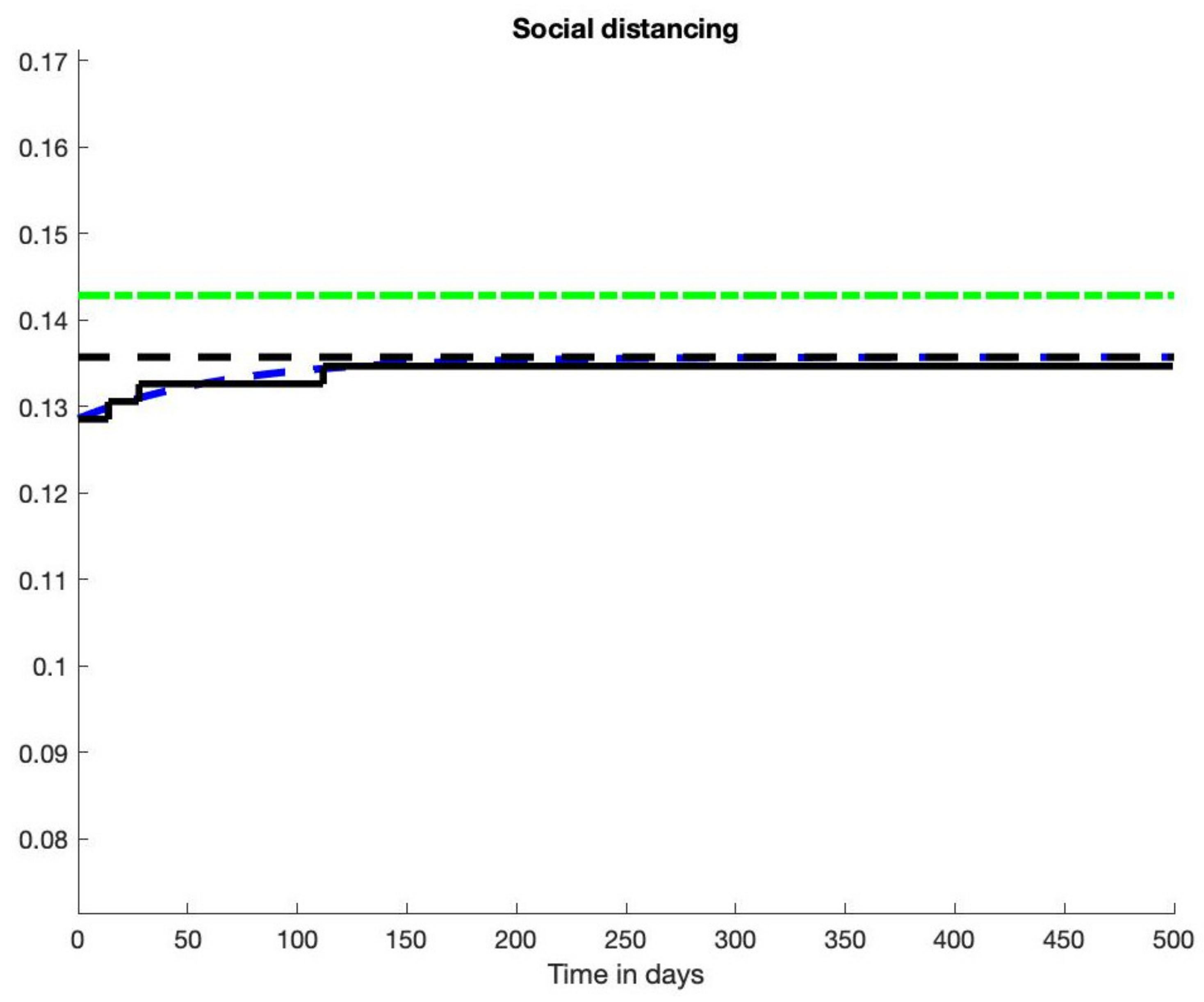
4.1.2. Scenario 2
4.2. Less Unrealistic Scenarios
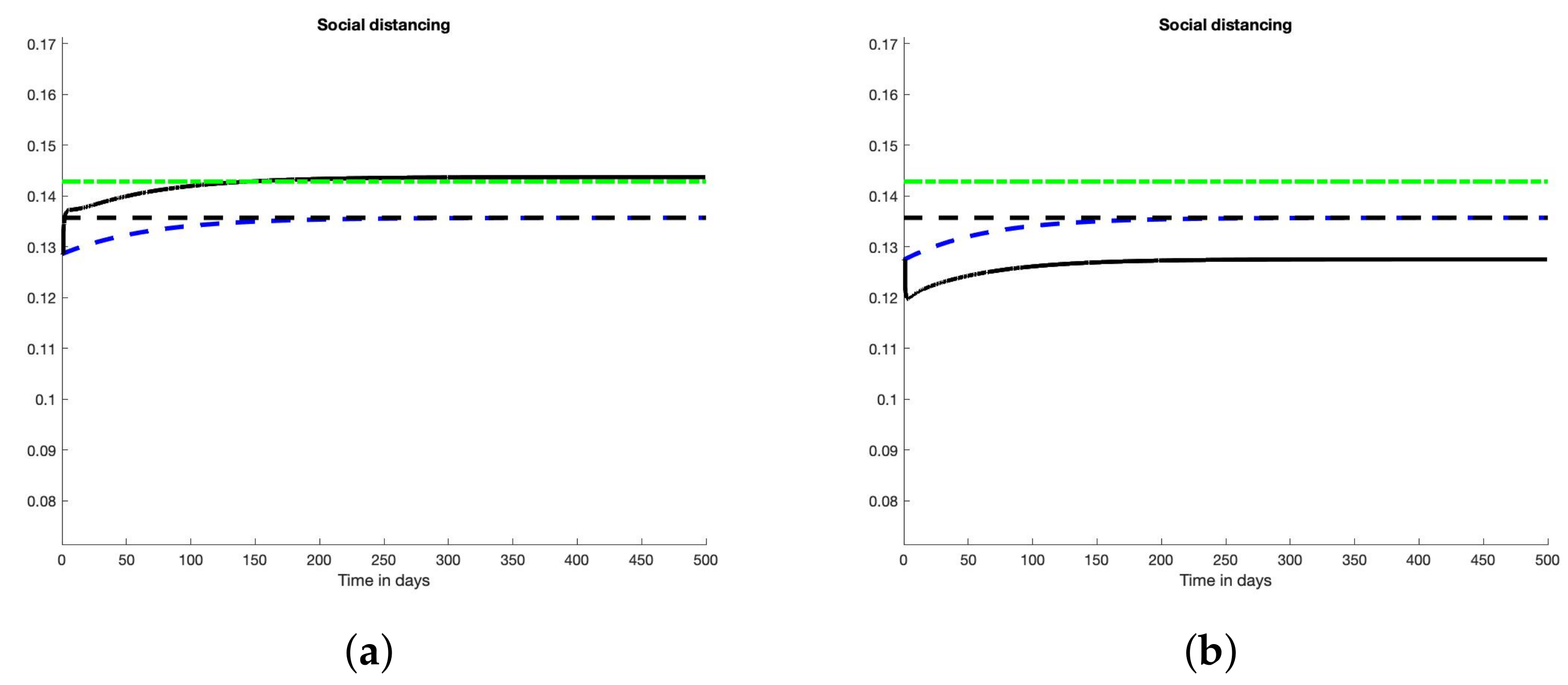
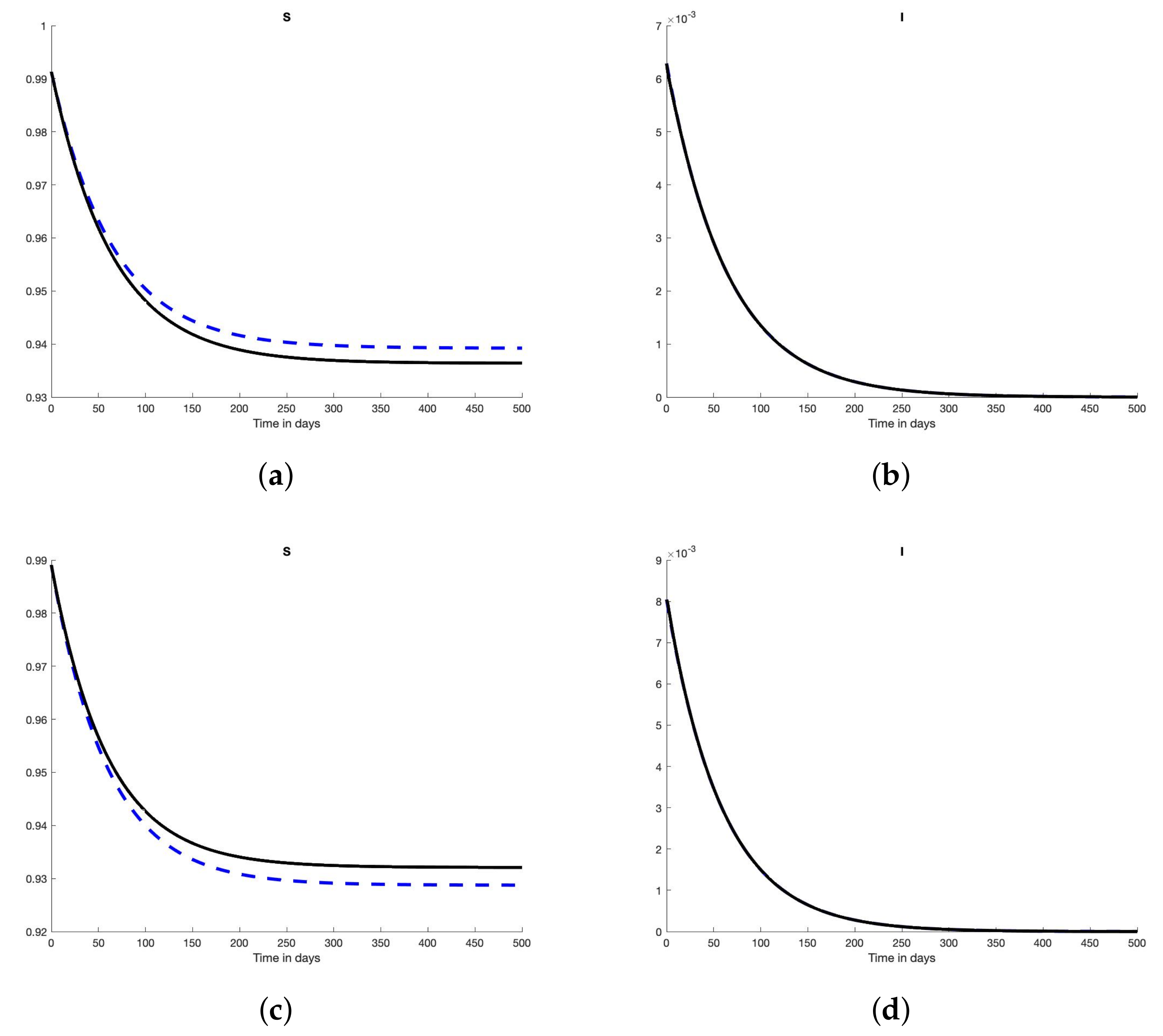
4.2.1. Scenario 3
4.2.2. Scenario 4
4.3. Scenarios 5–6: A More Realistic Policy
5. Conclusions
- continuous manipulations of non-pharmaceutical interventions, which are an obstacle to the implementation of the vast majority of theoretical control strategies in epidemiology, even for the remarkably different problem of vaccination awareness campaigns (see [67]), are avoided,
- severe and long lockdowns are replaced by more subtle alternations of more or less strict social distancing measures.
- Another interrogation is about the interpretation of the numerical values of the control variable . What is, for instance, the influence of closing nightclubs as done in France and elsewhere? Available estimation techniques would suffer from the poor knowledge of I, and therefore of R and S. This inefficiency includes the techniques employed in [18], where the assumed knowledge of I is unrealistic.
Author Contributions
Funding
Data Availability Statement
Conflicts of Interest
References
- Adolph, C.; Amano, K.; Bang-Jensen, B.; Fullman, N.; Wilkerson, J. Pandemic politics: Timing state-level social distancing responses to COVID-19. J. Health Polit. Policy Law 2021, 46, 211–233. [Google Scholar]
- Al-Radhawi, M.A.; Sadeghi, M.; Sontag, E.D. Long-term regulation of prolonged epidemic outbreaks in large populations via adaptive control: A singular perturbation approach. IEEE Contr. Syst. Lett. 2022, 6, 578–583. [Google Scholar]
- Ames, A.Z.; Molnár, T.G.; Singletary, A.W.; Orosz, G. Safety-critical control of active interventions for COVID-19 mitigation. IEEE Access 2020, 8, 188454–188474. [Google Scholar]
- Angulo, M.T.; Castanños, F.; Moreno-Morton, R.; Velasco-Hernández, J.X.; Moreno, J.A. A simple criterion to design optimal non-pharmaceutical interventions for mitigating epidemic outbreaks. J. Roy. Soc. Interface 2021, 18, 20200803. [Google Scholar]
- Berger, T. Feedback control of the COVID-19 pandemic with guaranteed non-exceeding ICU capacity. Syst. Contr. Lett. 2022, 160, 105111. [Google Scholar]
- Bisiacco, M.; Pillonetto, G. COVID-19 epidemic control using short-term lockdowns for collective gain. Ann. Rev. Contr. 2021, 52, 573–586. [Google Scholar]
- Bisiacco, M.; Pillonetto, G.; Cobelli, C. Closed-form expressions and nonparametric estimation of COVID-19 infection rate. Automatica 2022, 140, 110265. [Google Scholar]
- Bliman, P.-A.; Duprez, M. How best can finite-time social distancing reduce epidemic final size? J. Theoret. Biol. 2021, 511, 110557. [Google Scholar]
- Bliman, P.-A.; Duprez, M.; Privat, Y.; Vauchelet, N. Optimal immunity control and final size minimization by social distancing for the SIR epidemic model. J. Optim. Theory App. 2021, 189, 408–436. [Google Scholar]
- Bonnans, J.F.; Gianatti, J. Optimal control techniques based on infection age for the study of the COVID-19 epidemic. Math. Model. Nat. Phenom. 2020, 15, 48. [Google Scholar]
- Borri, A.; Palumbo, P.; Papa, F.; Possieri, C. Optimal design of lock-down and reopening policies for early-stage epidemics through SIR-D models. Ann. Rev. Contr. 2021, 51, 511–524. [Google Scholar]
- Charpentier, A.; Elie, R.; Laurière, M.; Tran, V.C. COVID-19 pandemic control: Balancing detection policy and lockdown intervention ICU sustainability. Math. Model. Nat. Phenom. 2020, 15, 57. [Google Scholar]
- Dias, S.; Queiroz, K.; Araujo, A. Controlling epidemic diseases based only on social distancing level. J. Contr. Autom. Electr. Syst. 2022, 33, 8–22. [Google Scholar]
- Di Lauro, F.; Kiss, I.Z.; Della Santina, C. Optimal timing of one-shot interventions for epidemic control. PLoS Comput. Biol. 2021, 17, e1008763. [Google Scholar]
- Di Lauro, F.; Kiss, I.Z.; Della Santina, C. Covid-19 and flattening the curve: A feedback control perspective. IEEE Contr. Syst. Lett. 2021, 5, 1435–1440. [Google Scholar]
- Efimov, D.; Ushirobira, R. On an interval prediction of COVID-19 development based on a SEIR epidemic model. Ann. Rev. Contr. 2021, 51, 477–487. [Google Scholar]
- Esterhuizen, W.; Lévine, J.; Streif, S. Epidemic management with admissible and robust invariant sets. PLoS ONE 2021, 16, e0257598. [Google Scholar]
- Fliess, M.; Join, C.; d’Onofrio, A. Feedback control of social distancing for COVID-19 via elementary formulae. In Proceedings of the 10th Vienna International Conference on Mathematical Modelling, MATHMOD 2022, Vienna, Austria, 27–29 July 2022; Available online: https://hal.archives-ouvertes.fr/hal-03547380/en/ (accessed on 6 April 2022).
- Gevertz, J.L.; Greene, J.M.; Sanchez-Tapia, C.H.; Sontag, E.D. A novel COVID-19 epidemiological model with explicit susceptible and asymptomatic isolation compartments reveals unexpected consequences of timing social distancing. J. Theoret. Biol. 2021, 510, 110539. [Google Scholar]
- Greene, J.M.; Sontag, E.D. Minimizing the infected peak utilizing a single lockdown: A technical result regarding equal peak. MedRxiv 2021. [Google Scholar] [CrossRef]
- Ianni, A.; Rossi, N. SIR-PID: A proportional-integral-derivative controller for COVID-19 outbreak containment. Physics 2021, 3, 459–472. [Google Scholar]
- Jing, M.; Yew Ng, K.; Mac Namee, B.; Biglarbeigi, P.; Brisk, R.; Bond, R.; Finlay, D.; McLaughlin, J. COVID-19 modelling by time-varying transmission rate associated with mobility trend of driving via Apple Maps. J. Biomed. Informat. 2021, 122, 103905. [Google Scholar]
- Köhler, J.; Schwenkel, L.; Koch, A.; Berberich, J.; Pauli, P.; Allgöwer, F. Robust and optimal predictive control of the COVID-19 outbreak. Ann. Rev. Contr. 2021, 51, 525–539. [Google Scholar]
- McQuade, S.T.; Weightman, R.; Merrill, N.J.; Yadav, A.; Trélat, E.; Allred, S.R.; Piccoli, B. Control of COVID-19 outbreak using an extended SEIR model. Math. Model. Meth. Appl. Sci. 2021, 31, 2399–2424. [Google Scholar]
- Morato, M.M.; Bastos, S.B.; Cajueiro, D.O.; Normey-Rico, J.E. An optimal predictive control strategy for COVID-19 (SARS-CoV-2) social distancing policies in Brazil. Ann. Rev. Contr. 2020, 50, 417–431. [Google Scholar]
- Morato, M.M.; Pataro, I.M.L.; da Costa, M.V.A.; Normey-Rico, J.E. A parametrized nonlinear predictive control strategy for relaxing COVID-19 social distancing measures in Brazil. ISA Trans. 2020, 124, 197–214. [Google Scholar] [CrossRef]
- Morgan, A.L.K.; Woolhouse, M.E.J.; Medley, G.F.; van Bunnik, B.A.D. Optimizing time-limited non-pharmaceutical interventions for COVID-19 outbreak control. Phil. Trans. Roy. Soc. B 2021, 376, 20200282. [Google Scholar]
- Morris, D.H.; Rossine, F.W.; Plotkin, J.B.; Levin, S.A. Optimal, near-optimal, and robust epidemic control. Communic. Phys. 2021, 4, 78. [Google Scholar]
- O’Sullivan, D.; Gahegan, M.; Exeter, D.J.; Adams, B. Spatially explicit models for exploring COVID-19 lockdown strategies. Trans. GIS 2020, 24, 967–1000. [Google Scholar]
- Péni, T.; Csutak, B.; Szederkényi, G.; Röst, G. Nonlinear model predictive control with logic constraints for COVID-19 management. Nonlin. Dyn. 2020, 102, 1965–1986. [Google Scholar]
- Pillonetto, G.; Bisiacco, M.; Palù, G.; Cobelli, C. Tracking the time course of reproduction number and lockdown’s effect on human behaviour during SARS-CoV-2 epidemic: Nonparametric estimation. Sci. Rep. 2021, 11, 9772. [Google Scholar]
- Sadeghi, M.; Greene, J.M.; Sontag, E.D. Universal features of epidemic models under social distancing guidelines. Ann. Rev. Contr. 2021, 51, 426–440. [Google Scholar]
- Sontag, E.D. An explicit formula for minimizing the infected peak in an SIR epidemic model when using a fixed number of complete lockdowns. Int. J. Robust Nonlin. Contr. 2021. [Google Scholar] [CrossRef]
- Stella, L.; Pinel Martínez, A.; Bauso, D.; Colaneri, P. The role of asymptomatic infections in the COVID-19 epidemic via complex networks and stability analysis. SIAM J. Contr. Optim. 2022, S119–S144. [Google Scholar]
- Tsay, C.; Lejarza, F.; Stadtherr, M.A.; Baldea, M. Modeling, state estimation, and optimal control for the US COVID-19 outbreak. Scientif. Rep. 2020, 10, 10711. [Google Scholar]
- Casella, F. Can the COVID-19 epidemic be controlled on the basis of daily test reports? IEEE Contr. Syst. Lett. 2021, 5, 1079–1084. [Google Scholar]
- Kermack, W.O.; McKendrick, A.G. A contribution to the mathematical theory of epidemics. Proc. R. Soc. Lond. Ser. A 1927, 115, 700–721. [Google Scholar]
- Brauer, F.; Castillo-Chavez, C. Mathematical Models in Population Biology and Epidemiology, 2nd ed.; Springer: New York, NY, USA, 2012. [Google Scholar]
- Hethcote, H.W. The mathematics of infectious diseases. SIAM Rev. 2020, 42, 599–603. [Google Scholar]
- Murray, J.D. Mathematical Biology I. An Introduction, 3rd ed.; Springer: Berlin/Heidelberg, Germany, 2002. [Google Scholar]
- Havers, F.P.; Reed, C.; Lim, T.; Montgomery, J.M.; Klena, J.D.; Hall, A.J.; Thornburg, N.J. Seroprevalence of antibodies to SARS-CoV-2 in 10 sites in the United States, March 23–May 12, 2020. JAMA Intern. Med. 2020, 180, 1576–1586. [Google Scholar]
- Pérez-Rechel, F.J.; Forbes, K.J.; Strachan, N.J.C. Importance of untested infectious individuals for interventions to suppress COVID-19. Nat. Sci. Rep. 2021, 11, 20728. [Google Scholar]
- Perkins, T.A.; Cavany, S.A.; Moore, S.M.; Oidtman, R.J.; Lerch, A.; Poterek, M. Estimating unobserved SARS-CoV-2 infections in the United States. Proc. Natl. Acad. Sci. USA 2020, 117, 22597–22602. [Google Scholar]
- Manfredi, P.; d’Onofrio, A. (Eds.) Modeling the Interplay Between Human Behavior and the Spread of Infectious Diseases; Springer: New York, NY, USA, 2013. [Google Scholar]
- Fliess, M.; Lévine, J.; Martin, P.; Rouchon, P. Flatness and defect of non-linear systems: Introductory theory and examples. Int. J. Contr. 1995, 61, 1327–1361. [Google Scholar]
- Fliess, M.; Lévine, J.; Martin, P.; Rouchon, P. A Lie-Bäcklund approach to equivalence and flatness of nonlinear systems. IEEE Trans. Automat. Contr. 1999, 44, 922–937. [Google Scholar]
- Lévine, J. Analysis and Control of Nonlinear Systems: A Flatness-Based Approach; Springer: Berlin/Heidelberg, Germany, 2009. [Google Scholar]
- Rigatos, G.G. Nonlinear Control and Filtering Using Differential Flatness Approaches—Applications to Electromechanical Systems; Springer: Berlin/Heidelberg, Germany, 2015. [Google Scholar]
- Rudolph, J. Flatness-Based Control: An Introduction; Shaker Verlag: Düren, Germany, 2021. [Google Scholar]
- Sira-Ramírez, H.; Agrawal, S.K. Differentially Flat Systems; Marcel Dekker: New York, NY, USA, 2004. [Google Scholar]
- Bonnabel, S.; Clayes, X. The industrial control of tower cranes: An operator-in-the-loop approach. IEEE Contr. Syst. Magaz. 2020, 40, 27–39. [Google Scholar]
- Guéry-Odelin, D.; Ruschhaupt, A.; Kiely, A.; Torrontegui, E.; Martínez-Garaot, S.; Muga, J.G. Shortcuts to adiabaticity: Concepts, methods, and applications. Rev. Mod. Phys. 2019, 91, 045001. [Google Scholar]
- Hametner, C.; Böhler, L.; Kozek, M.; Bartlechner, J.; Ecker, O.; Du, Z.P.; Kölbl, R.; Bergmann, M.; Bachleitner-Hofmann, T.; Jakubek, S. Intensive care unit occupancy predictions in the COVID-19 pandemic based on age-structured modelling and differential flatness. Nonlin. Dyn. 2022, 1–19. [Google Scholar] [CrossRef]
- Fliess, M.; Join, C.; Moussa, K.; Djouadi, S.M.; Alsager, M.W. Toward simple in silico experiments for drugs administration in some cancer treatments. IFAC PapersOnLine 2021, 54, 245–250. [Google Scholar]
- Villagra, J.; Herrero-Pérez, D. A comparison of control techniques for robust docking maneuvers of an AGV. IEEE Trans. Contr. Syst. Techno. 2012, 20, 1116–1123. [Google Scholar]
- Fliess, M.; Join, C. Model-free control. Int. J. Contr. 2013, 86, 2228–2252. [Google Scholar]
- Fliess, M.; Join, C. An alternative to proportional-integral and proportional-integral-derivative regulators: Intelligent proportional-derivative regulators. Int. J. Robust Nonlin. Contr. 2021. [Google Scholar] [CrossRef]
- Kuruganti, T.; Olama, M.; Dong, J.; Xue, Y.; Winstead, C.; Nutaro, J.; Djouadi, S.; Bai, L.; Augenbroe, G.; Hill, J. Dynamic Building Load Control to Facilitate High Penetration of Solar Photovoltaic Generation: Final Technical Report (No. ORNL/TM-2021/2112); Oak Ridge National Lab: Oak Ridge, TN, USA, 2021. [Google Scholar]
- Lv, M.; Gao, S.; Wei, Y.; Zhang, D.; Qi, H.; Wei, Y. Model-free parallel predictive torque control based on ultra-local model of permanent magnet synchronous machine. Actuators 2022, 11, 31. [Google Scholar]
- Michel, L.; Neunaber, I.; Mishra, R.; Braud, C.; Plestan, F.; Barbot, J.-P.; Boucher, X.; Join, C.; Fliess, M. Model-free control of the dynamic lift of a wind turbine blade section: Experimental results. J. Physics Conf. Series 2022, 2265, 032068. [Google Scholar]
- Sancak, C.; Yamac, F.; Itik, M.; Alici, G. Force control of electro-active polymer actuators using model-free intelligent control. J. Intel. Mater. Syst. Struct. 2021, 32, 2054–2065. [Google Scholar]
- Wang, Z.; Cosio, A.; Wang, J. Implementation resource allocation for collision-avoidance assistance systems considering driver capabilities. IEEE Trans. Intel. Transport. Syst. 2021. [Google Scholar] [CrossRef]
- Truong, C.T.; Huynh, K.H.; Duong, V.T.; Nguyen, H.H.; Pham, L.A.; Nguyen, T.T. Model-Free Vol. Press. Cycled Control Autom. Bag Valve Mask Vent. AIMS Bioengin. 2021, 8, 192–207. [Google Scholar]
- Åström, K.J.; Murray, R.M. Feedback Systems—An Introduction for Scientists and Engineers; Princeton University Press: Princeton, NJ, USA, 2008. [Google Scholar]
- Lafont, F.; Balmat, J.-F.; Pessel, N.; Fliess, M. A model-free control strategy for an experimental greenhouse with an application to fault accommodation. Comput. Electron. Agricult. 2015, 110, 139–149. [Google Scholar]
- Join, C.; Abouaïssa, H.; Fliess, M. Ramp metering: Modeling, simulation and control issues. In Advances in Distributed Parameter Systems; Auriol, J., Deutscher, J., Mazanti, G., Valmorbid, G., Eds.; Springer: Cham, Switzerland, 2022; pp. 227–242. [Google Scholar]
- Della Marca, R.; d’Onofrio, A. Volatile opinions and optimal control of vaccine awareness campaigns: Chaotic behaviour of the forward-backward sweep algorithm vs. heuristic direct optimization. Commun. Nonlin. Sci. Numer. Simulat. 2021, 98, 105768. [Google Scholar]
- Arruda, E.F.; Das, S.S.; Dias, C.M.; Pastore, D.H. Modelling and optimal control of multi strain epidemics, with application to COVID-19. PLoS ONE 2021, 16, e0257512. [Google Scholar]
- Kopfová, J.; Nábělková, P.; Rachinskii, D.; Rouf, S.C. Dynamics of SIR model with vaccination and heterogeneous behavioral response of individuals modeled by the Preisach operator. J. Math. Bio. 2021, 83, 11. [Google Scholar]
- Laguzet, L.; Turinici, G. Global optimal vaccination in the SIR model: Properties of the value function and application to cost-effectiveness analysis. Math. Biosci. 2015, 263, 180–197. [Google Scholar]
- Moore, S.; Hill, E.M.; Tildesley, M.J.; Dyson, L.; Keeling, M.J. Vaccination and non-pharmaceutical interventions for COVID-19: A mathematical modelling study. Lancet Infect. Dis. 2021, 21, 793–802. [Google Scholar]
- D’Onofrio, A.; Manfredi, P.; Salinelli, E. Vaccinating behaviour, information, and the dynamics of SIR vaccine preventable diseases. Theoret. Populat. Bio. 2007, 71, 301–317. [Google Scholar]
- Ramos, A.M.; Vela-Pérez, M.; Ferrández, M.R.; Kubik, A.B.; Ivorra, B. Modeling the impact of SARS-CoV-2 variants and vaccines on the spread of COVID-19. Commun. Nonlin. Sci. Numer. Simulat. 2021, 102, 105937. [Google Scholar]


Publisher’s Note: MDPI stays neutral with regard to jurisdictional claims in published maps and institutional affiliations. |
© 2022 by the authors. Licensee MDPI, Basel, Switzerland. This article is an open access article distributed under the terms and conditions of the Creative Commons Attribution (CC BY) license (https://creativecommons.org/licenses/by/4.0/).
Share and Cite
Join, C.; d’Onofrio, A.; Fliess, M. Toward More Realistic Social Distancing Policies via Advanced Feedback Control. Automation 2022, 3, 286-301. https://doi.org/10.3390/automation3020015
Join C, d’Onofrio A, Fliess M. Toward More Realistic Social Distancing Policies via Advanced Feedback Control. Automation. 2022; 3(2):286-301. https://doi.org/10.3390/automation3020015
Chicago/Turabian StyleJoin, Cédric, Alberto d’Onofrio, and Michel Fliess. 2022. "Toward More Realistic Social Distancing Policies via Advanced Feedback Control" Automation 3, no. 2: 286-301. https://doi.org/10.3390/automation3020015