State Machine Approach for Lane Changing Driving Behavior Recognition

Abstract

Research in understanding human behavior is a growing field within the development of Advanced Driving Assistance Systems (ADASs). In this contribution, a state machine approach is proposed to develop a driving behavior recognition model. The state machine approach is a behavior model based on the current state and a given set of inputs. Transitions to different states occur or we remain in the same state producing outputs. The transition between states depends on a set of environmental and driving variables. Based on a heuristic understanding of driving situations modeled as states, as well as one of the related actions modeling the state, using an assumed relation between them as the state machine topology, in this paper, a crisp approach is applied to adapt the model to real behaviors. An important aspect of the contribution is to introduce a trainable state machine-based model to describe drivers’ lane changing behavior. Three driving maneuvers are defined as states. The training of the model is related to the definition/tuning of transition variables (and state definitions). Here, driving data are used as the input for training. The non-dominated sorting genetic algorithm II is used to generate the optimized transition threshold. Comparing the data of actual human driving behaviors collected using driving simulator experiments and the calculated driving behaviors, this approach is able to develop a personalized behavior recognition model. The newly established algorithm presents an easy to apply, reliable, and interpretable AI approach.

1. Introduction

Traffic accidents within Germany have increased over the past few years. In the year 2019 alone, the Department of Statistics in Germany recorded that 74.4 percent of accidents were related to human driving error, such as inappropriate speed, insufficient space, and failure to yield the right of way [1]. Advanced Driving Assistance Systems (ADASs) have played an important role in assisting a human driver on the road to minimize errors while driving in recent years. Thus, developing a driving behavior prediction and recognition model is an important aspect in the development of ADASs. To improve driving predictions, this can be done by understanding individual driving behaviors to predict driving decisions in different environments. This improved ADAS model parameterized to individual driving preferences can inform the driver about suitable moves or how to maneuver accurately in different situations based on individual driving style by taking into account the safety and environmental conditions.

Developing driving prediction and recognition models has been previously tackled in several research works by using different machine learning algorithms such as in Gindele et al. [2], where the Dynamic Bayesian Network (DBN) was used in the context of predicting traffic situations. Unlabeled observations are used to learn a continuous, non-linear, context dependent process model for drivers. In Hurwitz et al. [3], empirical observed driving behaviors at a high speed signalized intersection area were used to develop a Fuzzy Logic (FL) model. The Hidden Markov Model (HMM) was used by Tran et al. [4] to predict different driving intentions such as changing lanes, turning directions, and stopping or not stopping. There are two common approaches used in this field: One combines two or more machine learning algorithms, such as in Mahajan et al. [5], where density-based clustering was used to identify lane changing maneuvers and a Support Vector Machine (SVM)-based model was then trained to label the new raw data automatically to predict the lane changing maneuvers. The other approach requires finding suitable input features using feature selection methods such as wrappers and filters, as done by Mostert et al. [6]. In previous works, related driving behavior prediction approaches were given in Deng et al. [7,8]. In Deng et al. [7], the authors used an improved HMM to predict the driving behaviors by introducing a prefilter. The comparison between using a general and optimal prefilter to estimate the driving behaviors was done to analyze the prediction accuracy. In [8], FL and HMM were combined to improve the driving prediction. A prefilter was proposed to process and combine signals to form suitable input features. This approach focuses on obtaining optimal prefilters of HMM and optimal thresholds of FL using the Non-dominated Sorting Genetic Algorithm II (NSGA-II) to improve the prediction performance. In this contribution, selecting optimal variables like brake pressure or Time To Collision (TTC) are important as these parameters affect the driving behavior prediction. Here, optimal denotes the solution idea solving the conflict between the accuracy and the false alarm sensitivity by applying NSGA-II for training. The aim in this research is to use a simpler method to produce similar results as previous works within this field.

In this contribution, a trainable and interpretable state machine-based approach is introduced for the first time as a machine learning algorithm applied to situation recognition. One of the advantages of this approach is that it is easy to track which event/data/condition is causing a change. The state machine systems are easy to design; hence, a quick implementation and execution are enabled. This is in contrast with other approaches (like Support Vector Machines (SVM)), whereby the final model and weights may be hard to interpret. Another advantage is that the state machine-based approach is flexible, enabling a finite state-based system using a topology. The state machine structure is able to determine the next possible state easily based on a set of conditions. One of the disadvantages of a state machine approach is that the approach may not be suitable to all types of dynamical systems; it can be used when a system has different states with defined and crisp conditions for state transition. This approach has already been applied in different research areas such as tribological experiments to describe a lifetime model expressing the relationship between wear degradation and Remaining Useful Lifetime (RUL) based on Acoustic Emission (AE) data for state selection [9]. In Jihin et al. [10], the state machine approach was used to correlate a lifetime model and the degradation states of a plant. Optimal parameters were defined using the NSGA-II for the optimization of the framework. The prediction of leaf elongation was carried out using the established model for performance evaluation [10]. Thus, here, the aim is to use this previously introduced approach as a simple, easy to understand new approach, which is interpretable within the traffic/automation field.

This contribution realizes this approach to estimate driving behaviors. Three driving behaviors, lane keeping, changing to the left, and changing to the right, are considered, defined as states. The estimation of driving behaviors relies on related parameters (thresholds of variables) and the conditions associated with them. One of the desired objectives of this contribution is to establish a driving behavior recognition model with respect to a high Accuracy (ACC), Detection Rate (DR), and low False Alarm Rate (FAR). Using the NSGA-II optimization framework, all parameters are defined by optimization.

This contribution is organized as follows: In Section 2, an overview of the state machine concept and the introduction and integration of the state machine approach in driving prediction experiments are presented. Here, the driving prediction model and the objective to compare the real driving behaviors and calculated driving behaviors using this model are described. In Section 2, the design of the experiment is shown. The results and evaluations are presented in Section 3. In Section 4, a discussion about this research work is presented. Finally, the conclusions, a summary, and the future work are provided in Section 5.

2. Materials and Methods

2.1. Methodology

To establish a driving behavior model, first the inputs and outputs of the considered system need to be defined. Lane changing, as an example of a driving maneuver, is selected as a representative of driving behaviors in this contribution. Three different driving maneuvers including Lane Keeping (LK), Lane Changing to the Left (LCL), and Lane Changing to the Right (LCR) are modeled as the outputs of the model. The variables affecting driver’s decisions are used as the inputs, assuming they are measurable. In general, different states of the ego vehicle (position, speed, acceleration, steering wheel angle, etc.) and information about surrounding vehicles are used as the inputs. The main aim is to establish a suitable recognition performance with respect to the ACC, DR, and FAR.

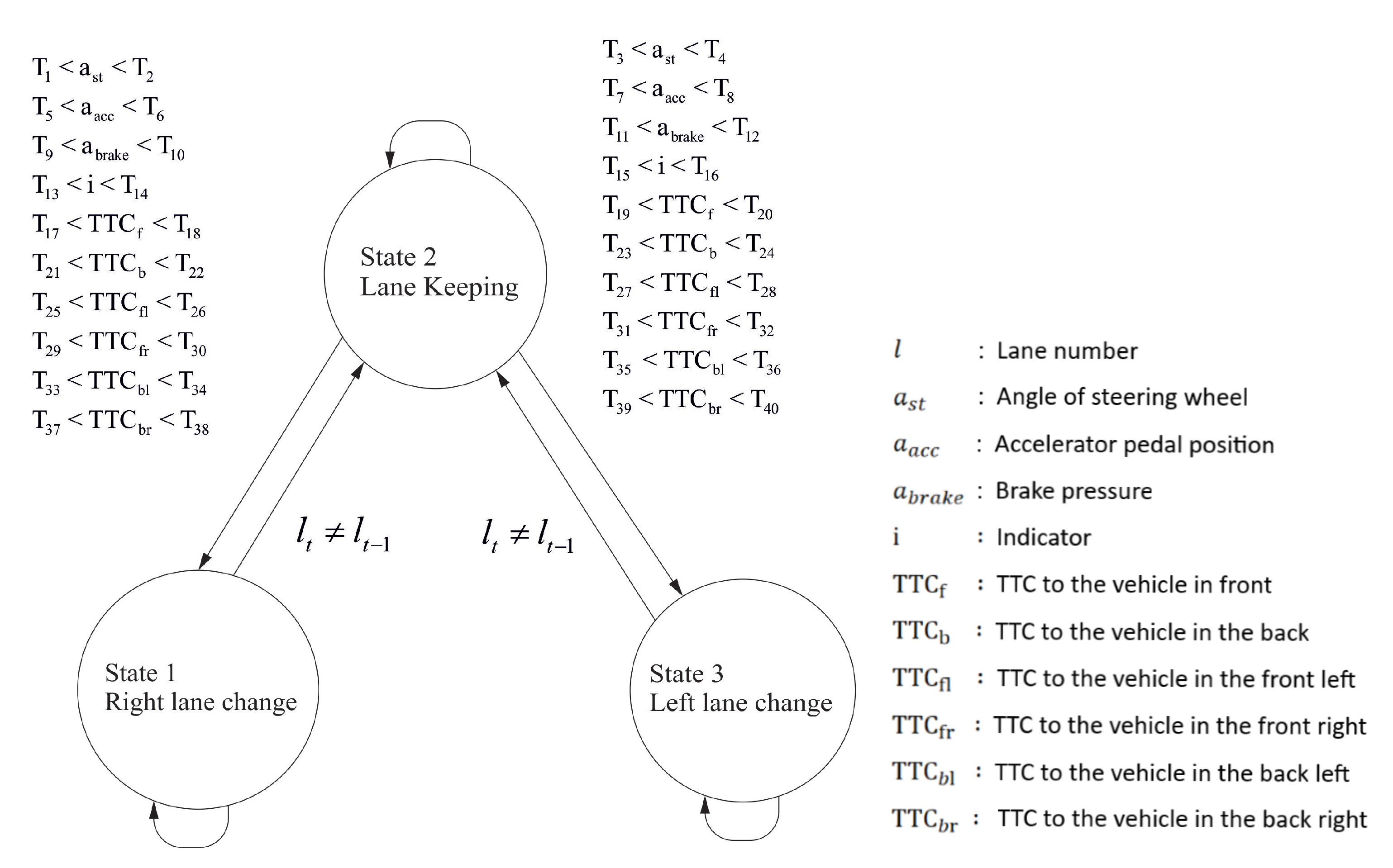
2.1.1. State Machine Approach

A state machine, in the case of deterministic modeling, models behaviors based on a set of inputs. Based on the inputs, the system dynamics are characterized by a sequence of transitions, whereby the system can either remain in the current state or shift to another state. State machines are well known approaches used for modeling, analysis, and control. In the classical approach, the parameters and variables used for modeling are defined by designers or are related to processes to be modeled or designed. The idea first published in Beganovic et al. [9] was using a state machine approach with parameters defining states and transitions (so, only the topology was given by designers first) as part of an optimization loop to develop models describing wear degradation behaviors. According to the given objectives, these parameters of the optimization variables were to be defined (using the NSGA-II) with the best/optimal parameters, using data from a tribological experiment.

2.1.2. Integration of the State Machine Approach in Driving Behavior Prediction

In this contribution, the state machine approach is assumed as given in Figure 1. Here, a state is defined as a driving behavior like “lane keeping” or “lane changing”, whereby it is assumed that the different states are connected by parameterized transitions. The topology shown consists of three states (driving behaviors) transitioning from one state to another based on specific parameter/threshold conditions generated by the NSGA-II. The parameters/thresholds are given in

Table 1. Description of the NSGA-II variables and related optimization thresholds.

Input	Variables	Design Parameters
$a_{st}$	Angle of steering wheel	[$T_1..T_2$] [$T_3..T_4$]
$a_{acc}$	Accelerator pedal position	[$T_5..T_6$] [$T_7..T_8$]
$a_{brake}$	Brake pedal pressure	[$T_9..T_{10}$] [$T_{11}..T_{12}$]
i	Indicator	[$T_{13}..T_{14}$] [$T_{15}..T_{16}$]
$TT{C}_f$	Time To Collision (TCC) with the vehicle in front	[$T_{17}..T_{18}$] [$T_{19}..T_{20}$]
$TT{C}_b$	TTC with the vehicle in the back	[$T_{21}..T_{22}$] [$T_{23}..T_{24}$]
$TT{C}_{fl}$	TTC with the vehicle in the front left	[$T_{25}..T_{26}$] [$T_{27}..T_{28}$]
$TT{C}_{fr}$	TTC with the vehicle in the front right	[$T_{29}..T_{30}$] [$T_{31}..T_{32}$]
$TT{C}_{bl}$	TTC with the vehicle in the back left	[$T_{33}..T_{34}$] [$T_{35}..T_{36}$]
$TT{C}_{br}$	TTC with the vehicle in the back right	[$T_{37}..T_{38}$] [$T_{39}..T_{40}$]

. The variables used are the lane number (l), angle of the steering wheel ($a_{st}$), accelerator pedal position ($a_{acc}$), brake pressure ($a_{br}$), indicator (i), Time To Collision (TTC) with the vehicle in front ($TT{C}_f$), TTC with the vehicle in the back ($TT{C}_b$), TTC with the vehicle in the front left ($TT{C}_{fl}$), TTC with the vehicle in the front right ($TT{C}_{fr}$), TTC with the vehicle in the back left ($TT{C}_{bl}$), and TTC with the vehicle in the back right ($TT{C}_{br}$). The variables used consist of environmental ($TT{C}_f$, $TT{C}_b$, $TT{C}_{fl}$, $TT{C}_{fr}$, $TT{C}_{bl}$, and $TT{C}_{br}$) and operational ($a_{st}$, $a_{acc}$, $a_{br}$, and i) variables. Driving behaviors highly depend on the current environmental conditions and individual driving styles. The relationship between the ego vehicle and surrounding vehicles affects the lane changing decisions; thus, the TTC variables are taken into account as environmental variables to predict lane changing behaviors. While driving environmental variables are used for predicting driving behaviors, drivers may make lane changes with sudden acceleration. Hence, operation variables are considered as well. In this case, when the vehicle is in State 2, denoted as Lane Keeping (LK), the model can switch to State 1, denoted as Lane Changing to the Right (LCR), or to State 3, denoted as Lane Changing to the Left (LCL), if the model satisfies a set of threshold conditions. When in State 1, the model can only switch to State 2. Similarly when in State 3, the transition is only possible to State 2. State 1 and State 3 can only switch to State 2 if the current lane is not the same as the previous time step. In Table 1, the first set of thresholds, for each variable, is used to define a transition from State 2 to State 1, while the second set of thresholds is used to define a transition from State 2 to State 3. For a transition from State 2 to State 1, the values of either one of the variables have to be within the first set of thresholds. For a transition from State 2 to State 3 to occur, the values of either one of the variables generated should be within the second set of thresholds. If these threshold conditions are not met, the state machine remains in the same state. In Table 1, $T_n$ denotes the threshold values, and the maximum number of thresholds/parameters is 40; hence, n = 40. In Figure 2, the highway scenario, showing different vehicle maneuvers, is illustrated. The figure shows that the vehicle is in a Lane Keeping state (LK) first, then the vehicle makes a Lane Change to the Left (LCL) and continues LK. The time at which a lane change occurs is defined as $t_{lane}$, while $t_{angle}$ is defined as the start time of a lane changing behavior by determining the last significant change of the angle of the steering wheel. The process of lane changing is defined as the time interval between $t_{lane}$ and $t_{angle}$.

2.2. Driving Behavior Model Based on the State Machine Approach

The state machine model introduced here has two major components. The first part consists of determining the thresholds (design parameters) through optimization. The second part focuses on determining/recognizing the driving states based on the optimal thresholds. These thresholds of the variables determine whether a state transition can occur. The driving behaviors determined using this model and the actual driving behavior (by a human driver) will be compared to evaluate the accuracy and reliability of this model.

2.2.1. Driving Behavior Prediction Problem

When driving on a highway, the driver’s decision is often based on the ego vehicle’s relationship with the surrounding vehicles. Decisions rely on an individual perception of environmental variables and their combination, like the velocity of the ego vehicle and the actual angle of the steering wheel. The variables used here are given in Table 1. The states considered here were described in the previous section. In this case, a four lane highway is considered. Since transitions from one state to another are dependent on the optimized thresholds of variables, these thresholds are generated with respect to the maximal DR, maximal ACC, and minimal FAR (or maximal 1-FAR) to evaluate the model. The ACC, DR, and FAR are determined based on True Positive (TP), False Positive (FP), True Negative (TN), as well as False Negative (FN) values. The True Positive (TP) is calculated based on the number of events when an estimated maneuver is positive (right lane change) and the actual maneuver is positive as well. The False Positive (FP) is based on the number of events when an estimated maneuver is positive, but the actual driving behavior is not [12]. This concept is applied to the True Negatives (TNs) and False Negatives (FNs) as well. Thus, this enables the evaluation of the well known metrics [13] Accuracy (ACC), Detection Rate (DR), and False Alarm Rate (FAR), given as:

$$\begin{array}{c}\hfill ACC=\frac{TP+TN}{TP+TN+FP+FN},\end{array}$$

(1)

$$\begin{array}{c}\hfill \hspace{1em}\hspace{1em}\hspace{1em}DR=\frac{TP}{TP+FN}, \mathrm{and}\end{array}$$

(2)

$$\begin{array}{c}\hfill \hspace{1em}\hspace{1em}\hspace{1em}\hspace{1em}FAR=\frac{FP}{TN+FP}.\end{array}$$

(3)

Suitable objective functions are selected to evaluate the optimization process by comparing the real states (the real driving behaviors) and the calculated states at each moment. In the state machine model introduced in this paper, the variables ACC, DR, and FAR are used to describe the objective functions with respect to minimizing the deviation between measured and estimated driving behaviors. The aim is to minimize the deviation between the calculated and real driving behaviors. The termination criteria are based on the maximum generation. The optimal values of the parameters are generated when the conditions are fulfilled, which will then be used to calculate the driving behaviors. The objective functions are defined as:

$$\begin{array}{c}\hfill \hspace{1em}\hspace{1em}{f}_1=(1-D{R}_{right})+FA{R}_{right},\end{array}$$

(4)

$$\begin{array}{c}\hfill f_2=(1-D{R}_{keep})+FA{R}_{keep}, \mathrm{and}\end{array}$$

(5)

$$\begin{array}{c}\hfill \hspace{1em}\hspace{1em}{f}_3=(1-D{R}_{left})+FA{R}_{left}.\end{array}$$

(6)

Equations (4)–(6) express the objectives in terms of the DR and FAR for each state.

2.2.2. State Machine-Based Problem Description

Optimal values of the variables and related optimization thresholds are generated using the NSGA-II. The NSGA-II model used in this contribution was proposed by Song et al. [14], which is used for multi-objective optimization consisting of three main features. The model uses an elitist preserving method and a diversity preserving method, which involves crowding distance, and highlights the non-dominated results [12,15,16]. Due to the conflicting objectives, the NSGA-II is used to handle the multi-objective problem presented. In

Table 2. Description of the NSGA-II options.

Parameter	Value
Maximum population	20
Maximum generation	50
Crossover fraction	10
Mutation fraction	1/number of variables = 1/40
Crossover variable	Intermediate 1.2
Mutation variable	Gaussian, 0.1, 0.05

, the list of arguments/inputs required for the NSGA-II are shown. The design parameters generated by the NSGA-II are used to minimize the objective function.

2.3. Application of the New Approach

In this section, the experimental setup, training, and testing of the data are suitably tuned. The optimal design parameters from the NSGA-II to develop the driving recognition model will be discussed.

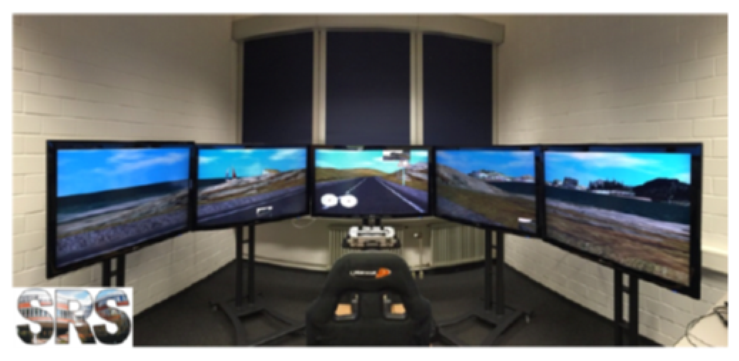
2.3.1. Design of Experiment

A driving simulator SCANeR^TM studio (Figure 3) was used to perform driving simulations to generate driving data. The simulator is equipped with five monitors, a base-fixed driver seat, a steering wheel, and pedals. The simulator also consists of three rear mirrors, which are essential to decide on a lane change. The mirrors are displayed on the corresponding positions of the monitors. The driving scenario is a highway with four lanes with two directions and a simulated traffic environment. During the driving, the participant can perform an overtaking maneuver when the preceding vehicle drives slowly. After overtaking, the driver can maneuver back to the initial lane. The time points of changing the lane to the left and right were decided by the participant. Following the traffic rules in Germany, it is only allowed to overtake from the left lane. The participants were allowed to make lane changes based on their choice and their assessment of the traffic situation. No further instructions were given such as the maximum number of vehicles they should overtake.

For the proof of concept, three datasets from three driving participants were used for training and testing. Each dataset (training and test) corresponds to a driver performing a driving scenario using the driving simulator. The training dataset is based on a forty minute drive by a participant, while the testing dataset is based on another ten minute drive by the same participant [8]. The training datasets and testing datasets contain different maneuvers. The current lane of the ego vehicle is determined through the vehicle’s center point. It is also worth mentioning that the driving and environmental conditions are normal (no fog, no rain, etc.). The driving and traffic conditions, as well as the scenarios are the same for all the drivers. The traffic condition are defined by the existence of different vehicles in the lane, and no further problems are generated.

2.3.2. Training and Test Procedure

Training phase: As mentioned previously, three different datasets are used. Further analysis has to be done to extend the approach to possibly structurally different driving behaviors. The datasets contain information about the current lane at each moment. The model is trained in the following manner:

• The NSGA-II generates transition parameters used in this experiment by using the training datasets.
• Based on the transition parameters, the driving behavior at each time point can be calculated based on the topology.
• Next, the calculated driving behaviors and the measured driving behaviors from the dataset are compared.
• This can be used to derive the ACC, DR, and FAR based on the calculated driving behavior.
• The values of the objective functions are derived.
• Processes (1) to (5) are repeated until convergence and the optimal model is obtained.

The training of datasets on a standard office PC (2.6 GHz) took around 26–68 s. The saved training results were then used for testing. The test process only took around 3–5 s for the algorithm to predict the driving behavior for different datasets. Based on the exemplary observed time, this is a very fast algorithm to execute. In addition, the training time is not linear to the dataset size, as each data point goes through ($50\times 20$) (population × generation) iterations in the NSGA-II optimization. In the test data, however, every data point is evaluated with a parameter generated from the training; hence, here, we have a linear relationship between the test time and the size of the data.

Test phase: The corresponding testing datasets are used here. The optimal values of the thresholds calculated from the training phase are used here to determine the driving behavior based on the test driving data. The ACC, DR, and FAR are determined by the calculated and actual driving behaviors.

3. Results

In this section, the results are presented. The driving behaviors generated using the state machine model will be shown and compared with the measured driving behaviors to check for similarities.

Figures, Tables, and Schemes

Here, results based on three datasets from three participants are shown. The datasets are generated from driving simulator experiments conducted in the driving simulator laboratory at the Chair of Dynamics and Control at University of Duisburg-Essen. As mentioned previously, the training dataset is based on a 40 min drive, while the testing dataset is based on a 10 min drive. The experiments were conducted with driving participants with ages from 25 to 38 years. All participants held a valid driving license. The best results are defined as those results generated from the tuned model showing the closest fit to the actual driving behaviors. The results in Figure 4, Figure 5 and Figure 6 are based on Testing Datasets 1, 2, and 3 when training their respective training datasets. In the ordinate, the y-axis represents the three different states, while the x-axis represents time, in seconds. The blue line represents the estimated driving behavior (or calculated states), and the red dotted line represents the driving behavior from the driving simulator.

In Figure 4, the estimated and measured driving behavior lines have a close fit with Testing Dataset 1 for most of the behaviors with some inconsistencies.

In Figure 5, the results are based on Training Dataset 2 and Testing Dataset 2. The results show a close fit for most of the states.

The results shown in Figure 6, are based on Training Dataset 3 and Testing Dataset 3. A close fit to the measured driving behavior can also be observed.

All figures show different lane changing behaviors. The driver makes the choice of staying in the same lane or makes a lane change based on assessing the traffic situation. The driver may steer to alternative lanes even if the current lane is free or may stay in the same lane even if there is a vehicle in front of the ego vehicle based on his/her free will. Besides lane changing behaviors, the input variables given in Table 1 change throughout the driving for each driver.

The ACC, DR, and FAR values for each state when training different datasets and the corresponding test data are shown in

Table 3. Recognition results for different training/test data combinations (here: Training Dataset 1, Testing Datasets 1–3).

Objectives (%)	Training Dataset 1	Testing Dataset 1	Dataset 2	Dataset 3
$AC{C}_{overall}$	91.90	92.90	95.30	91.69
$AC{C}_{right}$	95.03	96.02	97.70	98.61
$D{R}_{right}$	90.64	88.94	73.27	87.07
$FA{R}_{right}$	4.76	3.32	1.41	0.82
$AC{C}_{keep}$	92.11	93.11	95.37	92.08
$D{R}_{keep}$	92.13	93.32	97.37	91.99
$FA{R}_{keep}$	8.11	8.88	22.31	7.11
$AC{C}_{left}$	96.66	96.66	97.53	93.23
$D{R}_{left}$	88.69	88.76	80.75	95.92
$FA{R}_{left}$	2.94	2.94	1.58	6.92

,

Table 4. Recognition results for different training/test data combinations (here: Training Dataset 2, Testing Datasets 1–3).

Objectives (%)	Dataset 1	Training Dataset 2	Testing Dataset 2	Dataset 3
$AC{C}_{overall}$	92.89	93.08	95.77	91.69
$AC{C}_{right}$	96.22	94.97	97.48	98.56
$D{R}_{right}$	86.93	83.82	79.31	86.01
$FA{R}_{right}$	3.32	4.35	1.41	0.82
$AC{C}_{keep}$	93.05	93.22	95.97	91.93
$D{R}_{keep}$	93.40	94.12	97.22	91.74
$FA{R}_{keep}$	10.23	13.74	13.74	6.30
$AC{C}_{left}$	96.45	97.97	98.08	92.88
$D{R}_{left}$	88.66	86.22	89.78	95.92
$FA{R}_{left}$	3.15	1.33	1.42	7.28

and

Table 5. Recognition results for different training/test data combinations (here: Training Dataset 3, Testing Datasets 1–3).

Objectives (%)	Dataset 1	Dataset 2	Training Dataset 3	Testing Dataset 3
$AC{C}_{overall}$	92.69	95.30	91.76	93.35
$AC{C}_{right}$	96.22	97.70	98.62	96.22
$D{R}_{right}$	86.93	73.27	86.10	91.55
$FA{R}_{right}$	3.32	0.98	0.74	1.12
$AC{C}_{keep}$	92.97	95.37	91.91	93.35
$D{R}_{keep}$	93.40	97.37	91.70	93.74
$FA{R}_{keep}$	12.11	22.31	6.20	11.04
$AC{C}_{left}$	96.30	97.53	92.99	94.75
$D{R}_{left}$	85.28	80.75	98.18	86.80
$FA{R}_{left}$	3.14	1.58	7.29	4.88

. The ACC, DR, and FAR values given correspond to the datasets tested.

In Table 3, Training Dataset 1 it is tested with Testing Dataset 1, Training Dataset 1 (used for the test as well), Dataset 2 (a combination of Training and Testing Dataset 2), and Dataset 3 (a combination of Training and Testing Dataset 3) to show the generalizability and transferability.

In Table 4, Training Dataset 2 is tested with Testing Dataset 2, Training Dataset 2 (used for the test as well), Dataset 1 (a combination of Training and Testing Dataset 1), and Dataset 3 (a combination of Training and Testing Dataset 3).

In Table 5, Training Dataset 3 is tested with Testing Dataset 3, Training Dataset 3 (used for the test as well), Dataset 1 (a combination of Training and Testing Dataset 1) and Dataset 2 (a combination of Training and Testing Dataset 2).

4. Discussion

In this section, the validity of the results and the method used will be discussed. The state machine approach is established in this contribution first to recognize/predict driving behaviors. One of the objectives of this research is to develop a suitable driving recognition model by generating the optimal thresholds of variables using the NSGA-II. The other objective is to develop a close fit between the measured driving behaviors and generated behaviors from the model. The driving behavior considered here is lane changing behavior [8,17,18].

The results generally show a good fit between the behaviors for the datasets used. This method produces high ACC and DR and low FAR for most of the states. For an example, in Table 3, the overall accuracy for Testing Dataset 1 is 92.90%, with the highest left maneuver accuracy of 96.66% and low false alarm rates for all maneuvers. The overall accuracy for Testing Dataset 2 is the highest in comparison to the other datasets with an accuracy of 95.77%. A high accuracy of the left maneuver at 98.08% is achieved, which is not only the highest within the Testing Dataset 2, but also the highest value when compared with other testing datasets. However, the false alarm rate for lane keeping in Testing Dataset 2 is higher than the rest of the maneuvers within this dataset. The same can be said regarding the FAR for lane keeping in Testing Datasets 1 and 3. On the other hand, the FAR for the right and left maneuvers for Testing Dataset 2 is low at 1.41% and 1.42%, respectively. The detection rate also seems to perform well for the different maneuvers in all the datasets, with values larger than 73%. The results from this contribution generally show a close resemblance to the results from previous works [7,8]. The newly introduced approach is therefore easier to understand and, from the machine learning perspective, interpretable.

To verify the effectiveness of this method, the results developed in this paper are compared with the results developed using other techniques. In Deng et al. [8], who used the same dataset as this work, the average values of the ACC, DR, and (1-FAR)were higher than 80%. Here, the values of the ACC, DR, and (1-FAR) from the datasets are also generally higher than 80%, with some exceptions; for example, for Training Dataset 2, the DR for the right maneuver in Testing Dataset 2 is 79.31%. In contrast to Deng et al. [8], the main advantage of the approach introduced in this contribution is that the approach is interpretable, which is not the case for all the approaches applied by Deng et al. [8].

5. Conclusions

In this contribution, a state machine approach is introduced for driving behavior recognition/prediction. A topology is developed based on the transition of states by applying threshold-based conditions as the model parameters to be trained using the NSGA-II [19,20]. These transition parameters are determined by optimization. This allows the optimization to define those model parameters that fit best to the whole driving behavior sequence. To validate this model, three training and testing datasets are used and combined in the sense of cross-validation. The results show that the dataset trained and the dataset used for testing allow a close fit with acceptable accuracies. The ACC, DR, and FAR of the datasets are also evaluated to validate the efficiency of this model. Due to the fact that only three suitable datasets are used, it can be concluded that this machine learning-based approach may be also a new candidate for situation and driver behavior recognition and prediction in the future. Improvements, especially to the robustness with respect to different individual driving patterns, are required.

References

1. Statistisches Bundesamt (Destatis) Home Page. Available online: https://www.destatis.de/EN/Themes/Society-Environment/Traffic-Accidents/_Graphic/_Interactive/traffic-accidents-driver-related-causes.html (accessed on 15 July 2020).
2. Gindele, T.; Brechtel, S.; Dillmann, R. Learning context sensitive behavior models from observations for predicting traffic situations. In Proceedings of the 16th International IEEE Conference on Intelligent Transportation Systems (ITSC 2013), The Hague, The Netherlands, 6–9 October 2013; pp. 1764–1771. [Google Scholar]
3. Hurwitz, D.S.; Wang, H.; Knoldler, M.A., Jr.; Ni, D.; Moore, D. Fuzzy sets to describe driver behavior in the dilemma zone of high-speed signalized intersections. Transp. Res. Part F Traffic Psychol. Behav. 2012, 15, 132–143. [Google Scholar] [CrossRef]
4. Tran, D.; Sheng, W.; Liu, L.; Liu, M. A Hidden Markov Model based driver intention prediction system. In Proceedings of the 5th Annual IEEE International Conference on Cyber Technology in Automation, Control and Intelligent Systems Psychology and Behaviour (CYBER 2015), Shenyang, China, 8–12 June 2015; pp. 112–120. [Google Scholar]
5. Mahajan, V.; Katrakazas, C.; Antoniou, C. Prediction of Lane-Changing Maneuvers with Automatic Labeling and Deep Learning. Transp. Res. Rec. 2020, 2764, 336–347. [Google Scholar] [CrossRef]
6. Mostert, W.; Malan, K.; Engelbrecht, A. Filter Versus Wrapper Feature Selection Based on Problem Landscape Features, Genetic and Evolutionary Computation Conference; Association for Computing Machinery: New York, NY, USA, 2018; pp. 1489–1496. ISBN 9781450357647. [Google Scholar]
7. Deng, Q.; Wang, J.; Söffker, D. Prediction of human driver behaviors based on an improved HMM approach. In Proceedings of the IEEE Intelligent Vehicles Symposium (IV), Changshu, China, 26–30 June 2018; pp. 2066–2071. [Google Scholar]
8. Deng, Q.; Söffker, D. Improved driving behaviors prediction based on Fuzzy Logic-Hidden Markov Model (FL-HMM). In Proceedings of the IEEE Intelligent Vehicles Symposium (IV), Changshu, China, 26–30 June 2018; pp. 2003–2008. [Google Scholar]
9. Beganovic, N.; Söffker, D. Remaining lifetime modeling using State-of-Health estimation. Mech. Syst. Signal Process. 2017, 92, 107–123. [Google Scholar] [CrossRef]
10. Jihin, R.; Kogler, F.; Söffker, D. Data Driven State Machine Model for Industry 4.0 Lifetime Modeling and Identification of Irrigation Control Parameters. In Proceedings of the 3rd Global IoT Summit (GIoTS 2019), Aarhus, Denmark, 17–21 June 2019; pp. 1–6. [Google Scholar]
11. Deng, Q.; Söffker, D. Classifying Human Behaviors: Improving Training of Conventional Algorithms. In Proceedings of the IEEE Intelligent Transportation Systems Conference (ITSC), Auckland, New Zealand, 27–30 October 2019; pp. 1060–1065. [Google Scholar]
12. Calle, P. Analytics Lab at University of Oklahoma Home Page. Available online: http://oklahomaanalytics.com/data-science-techniques/nsga-ii-explained/ (accessed on 8 March 2020).
13. Mukhopadhyay, A.; Maulik, U.; Bandyopadhyay, S.; Coello, C.A.C. A Survey of Multiobjective Evolutionary Algorithms for Data Mining: Part I. IEEE Trans. Evol. 2014, 18, 4–19. [Google Scholar] [CrossRef]
14. Song, L. MathWorks Home Page. Available online: http://www.mathworks.com/matlabcentral/fileexchange/31166-ngpm-a-nsga-ii-program-inmatlab-v1-4 (accessed on 19 November 2019).
15. Deb, K. Multi-Objective Optimization Using Evolutionary Algorithms; John Wiley & Sons: New York, NY, USA, 2001; ISBN 978-0-471-87339-6. [Google Scholar]
16. Deb, K.; Pratap, A.; Agarwal, S.; Meyarivan, T. A Fast and Elitist Multiobjective Genetic Algorithm: NSGA-II. IEEE Trans. Evol. Comput. 2002, 6, 182–197. [Google Scholar] [CrossRef] [Green Version]
17. Kumar, P.; Perrollaz, M.; Lefevre, S.; Laugier, C. Learning-Based Approach for Online Lane Change Intention Prediction. In Proceedings of the IEEE Intelligent Vehicles Symposium, Gold Coast, Australia, 23–26 June 2013; pp. 797–802. [Google Scholar]
18. Hurwitz, D.S.; Knodler, M.A., Jr.; Nyquist, B. Evaluation of driver behavior in type II dilemma zones at high-speed signalized intersections. J. Transp. Eng. 2011, 137, 277–286. [Google Scholar] [CrossRef]
19. Goldberg, D.E. Genetic Algorithms in Search, Optimization and Machine Learning, 1st ed.; Addison-Wesley Longman Publishing Co., Inc.: Boston, MA, USA, 1989; ISBN 978-0-201-15767-3. [Google Scholar]
20. Bielser, D.; Glardon, P.; Teschner, M.; Gross, M. A state machine for real-time cutting of tetrahedral meshes. In Proceedings of the 11th Pacific Conference on Computer Graphics and Applications, Canmore, AB, Canada, 8–10 October 2003; pp. 377–386. [Google Scholar]
Figure 1. State machine topology for driving behavior prediction. TTC, Time To Collision.
Automation 01 00006 g001
Figure 2. Driving scenario on the highway [11].
Automation 01 00006 g002
Figure 3. State machine topology for the driving behavior prediction (Chair of Dynamics and Control, U DuE, Germany).
Automation 01 00006 g003
Figure 4. Comparison of calculated and measured driving states (Training Dataset 1, Testing Dataset 1).
Automation 01 00006 g004
Figure 5. Comparison of calculated and measured driving states (Training Dataset 2, Testing Dataset 2).
Automation 01 00006 g005
Figure 6. Comparison of calculated and measured driving states (Training Dataset 3, Testing Dataset 3).
Automation 01 00006 g006