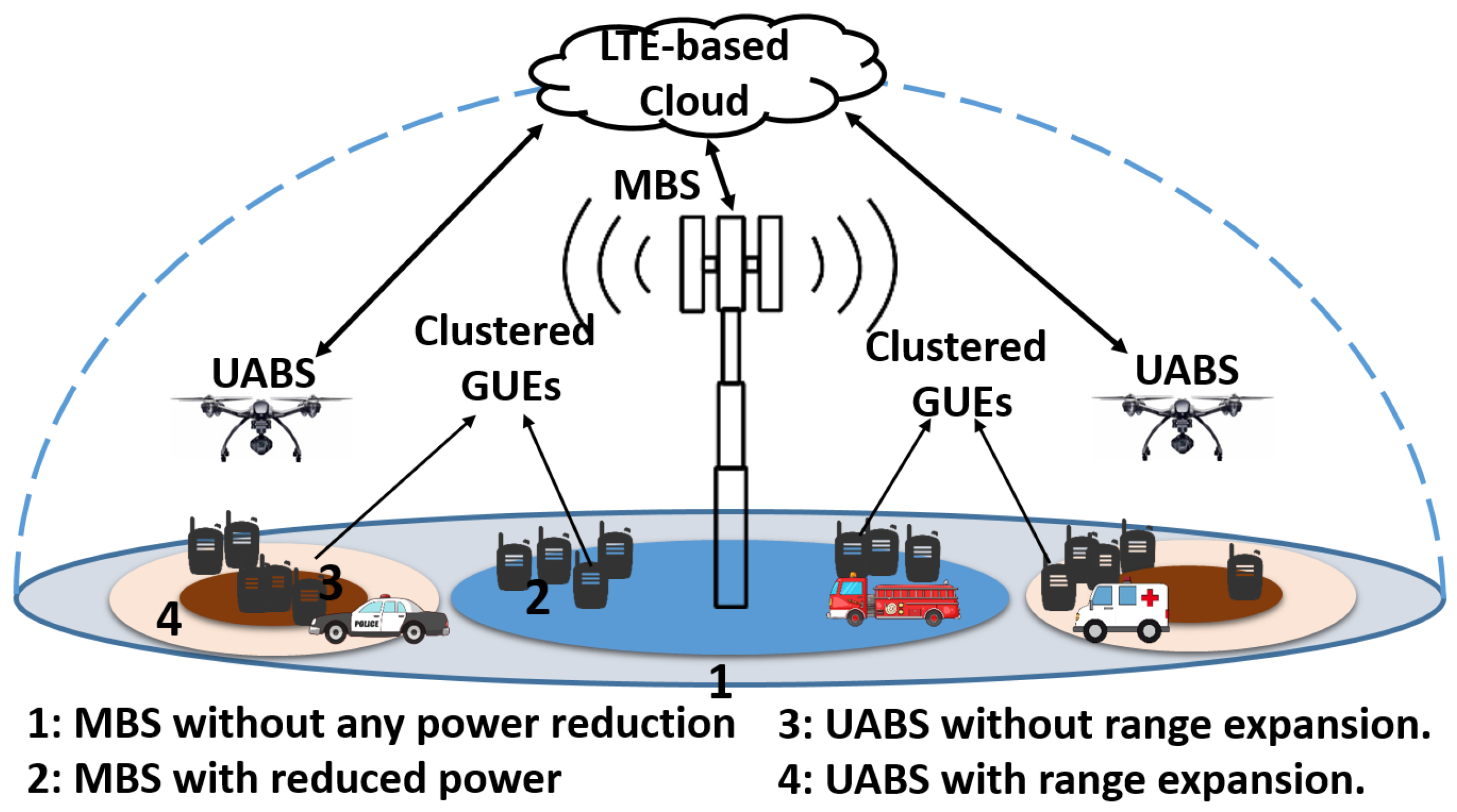
Figure 1.
An illustration of a PSC scenario with fixed MBS, mobile UABSs, and clustered GUEs constitute the air–ground HetNet infrastructure. The MBS can use various inter-cell interference coordination techniques defined in LTE-Advanced. The UABSs can utilize range expansion bias to offload GUEs from MBS.
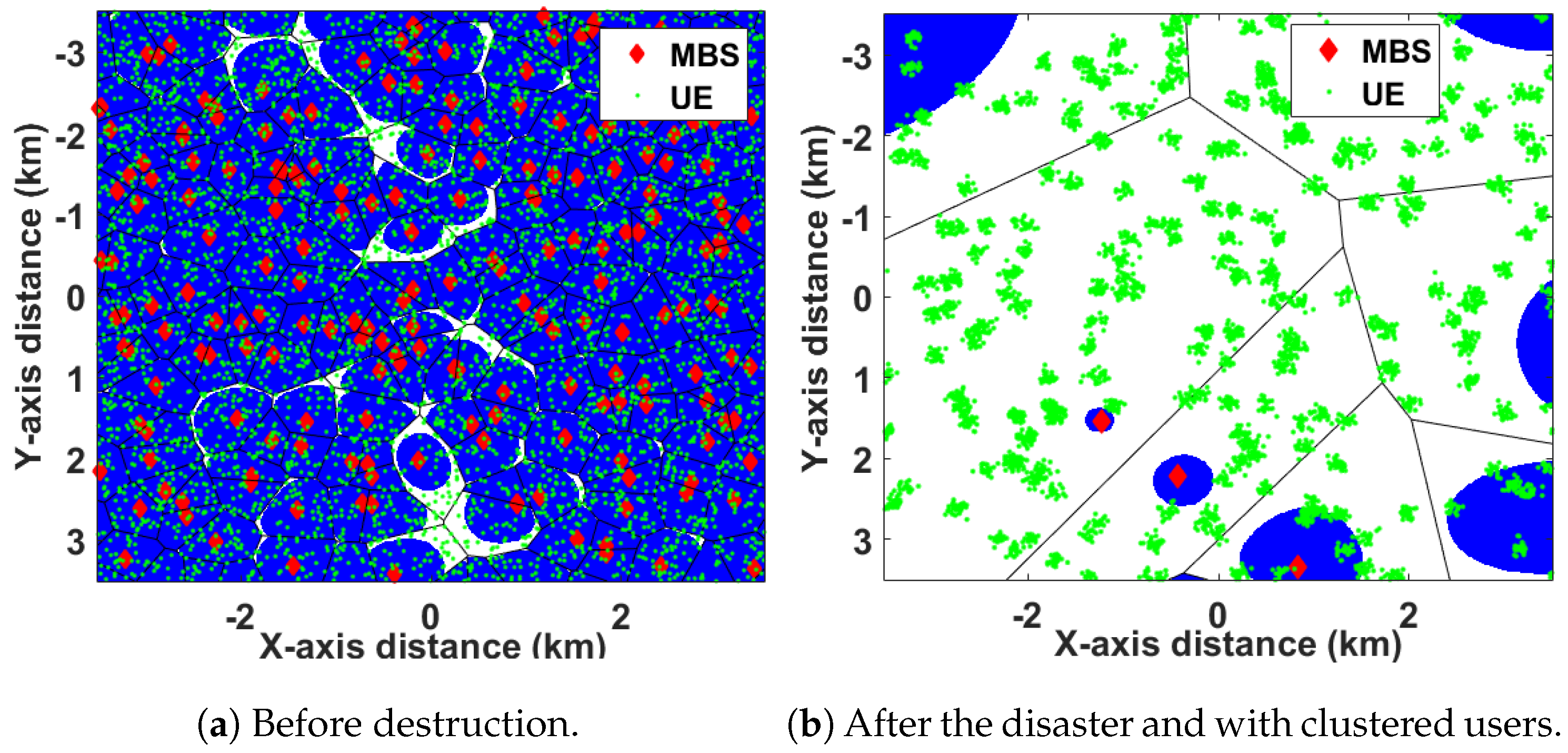
Figure 2.
Illustration of Typical PSC AG-HetNet and SE coverage before/after a disaster.
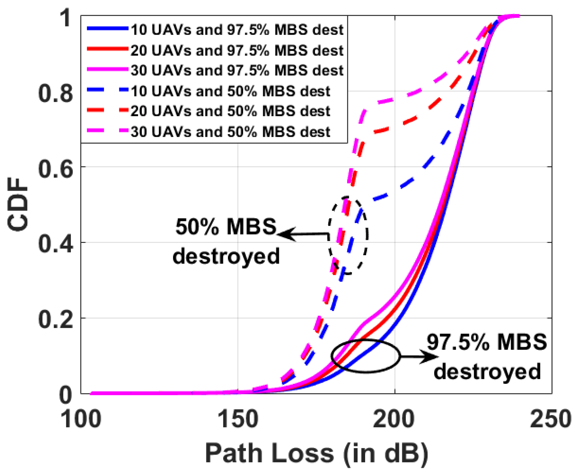
Figure 3.
The CDF describes the combined path loss observed from all the base stations in PSC AG-HetNet. The dashed lines correspond to the scenario where of the MBSs are destroyed, while solid lines correspond to the scenario with of the MBSs being destroyed. The CDF is plotted for GUEs distribution using the Matern and Thomas clusters processes.
Figure 4.
Illustration of LTE-Advanced frame structures for time-domain ICIC techniques, i.e., almost blank subframes (ABS) with is the 3GPP Release-10 eICIC, is the reduced power, and ABS (RP-ABS) is the 3GPP Release-11 FeICIC.
Figure 5.
Cell selection, association, and handover of GUEs in coordinate and uncoordinated radio subframes for all base stations in the AG-HetNet.
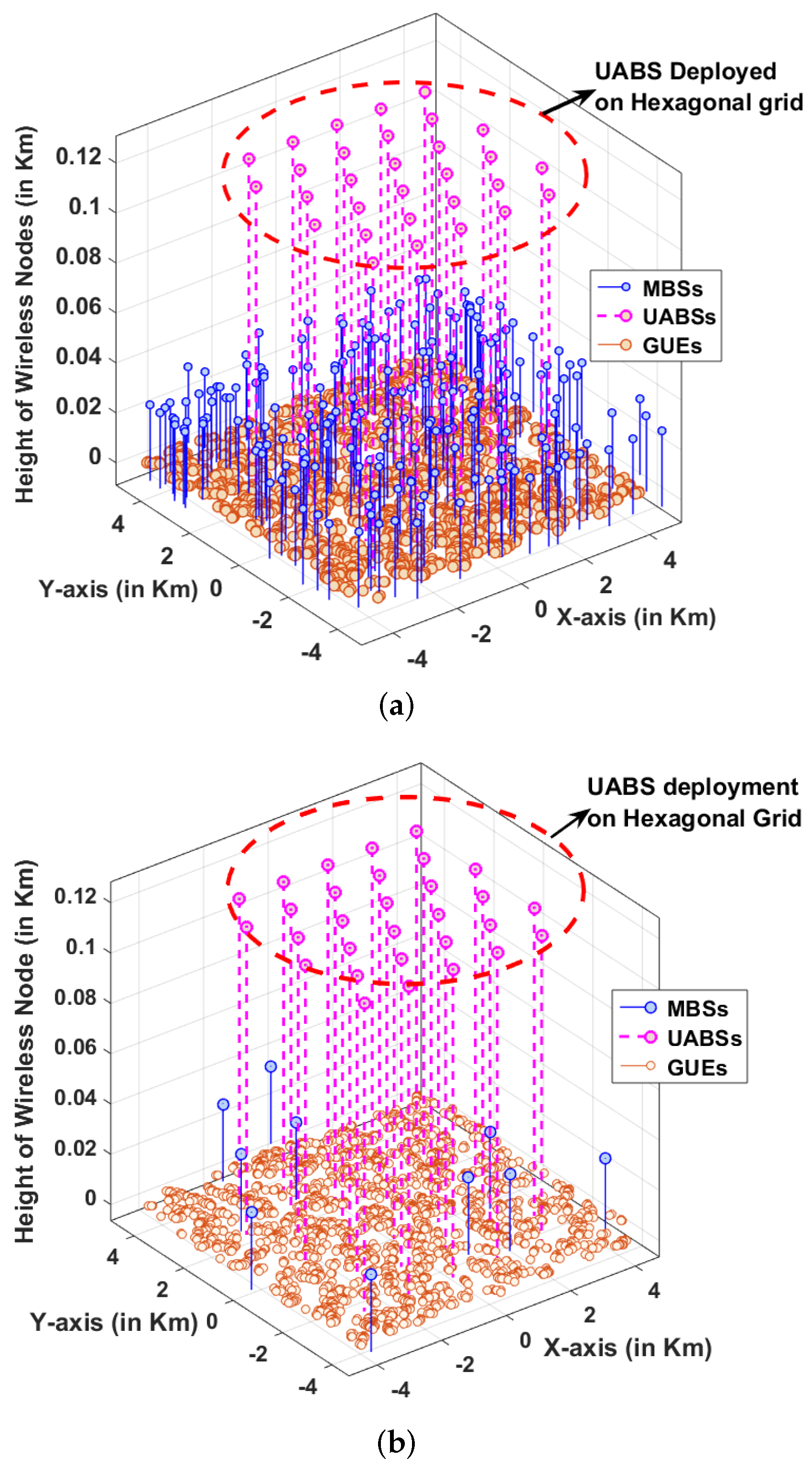
Figure 6.
Illustration of PSC network after a disaster and UABSs deployed to restore mission-critical communications. (a) Illustration of PSC network after a disaster, with 50% of the infrastructure destroyed and UABSs deployed on a fixed hexagonal grid and at the height of 120 m. (b) Illustration of PSC network after a disaster, with 95% of the infrastructure destroyed and UABSs deployed on a fixed hexagonal grid and at the height of 120 m.
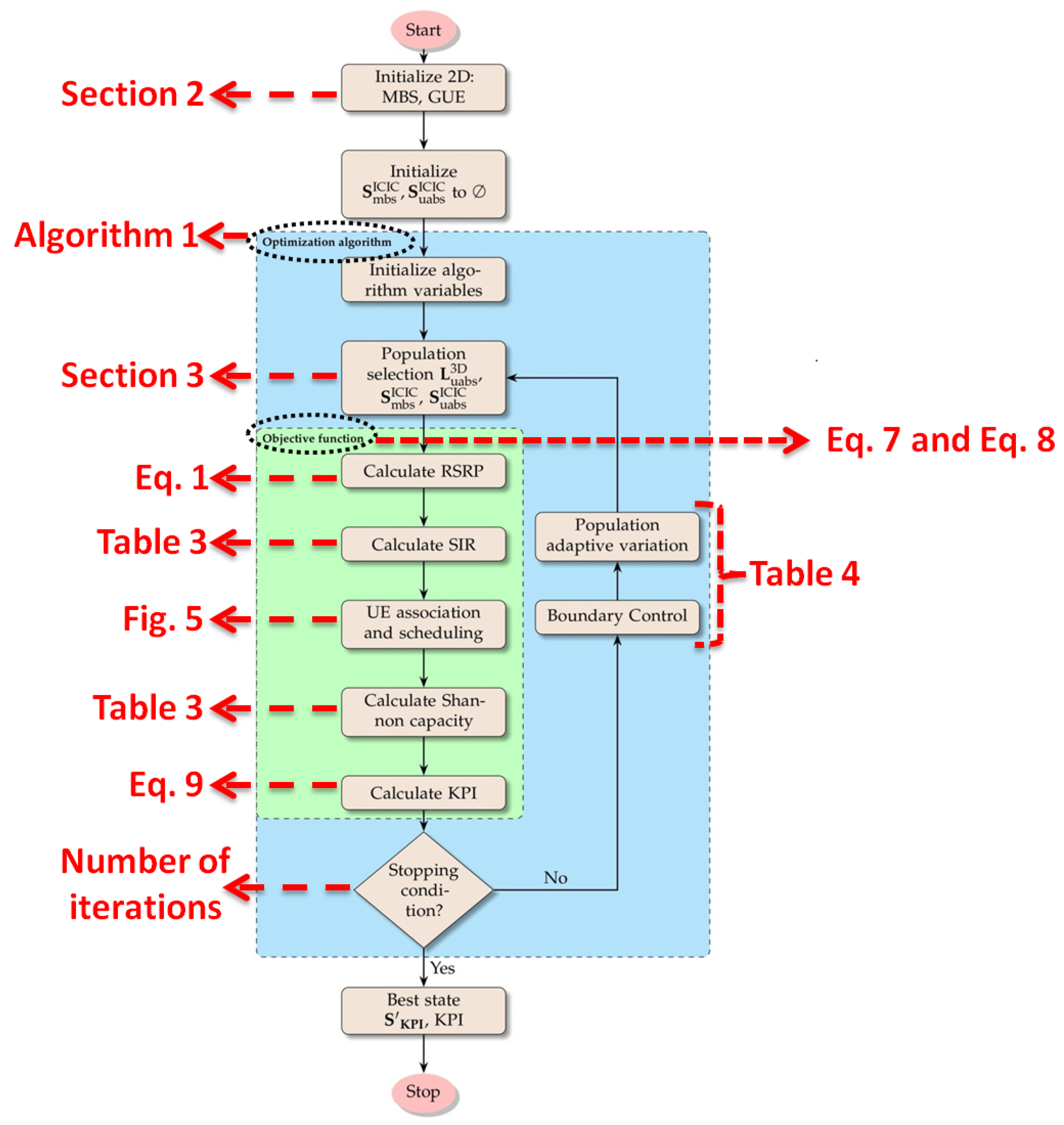
Figure 7.
A flowchart combining AG-HetNet system flow and the Brute Force algorithm used.
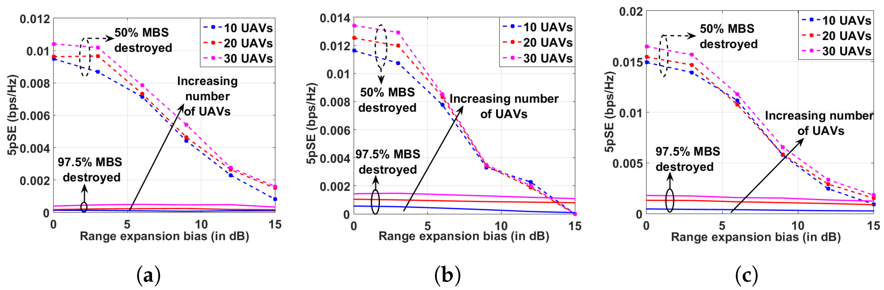
Figure 8.
Peak 5pSE performance of the wireless network, when GUEs are distributed using MCP, UABS deployed on a fixed hexagonal grid, and for different ICIC techniques. (a) NIM Peak 5pSE vs. CRE. (b) eICIC Peak 5pSE vs. CRE. (c) FeICIC Peak 5pSE vs. CRE.
Figure 9.
Peak coverage performance of the wireless network, when GUEs are distributed using MCP, UABS deployed on a fixed hexagonal grid, and for different ICIC techniques. (a) NIM Coverage probability vs. CRE. (b) eICIC Coverage probability vs. CRE. (c) FeICIC Coverage probability vs. CRE.
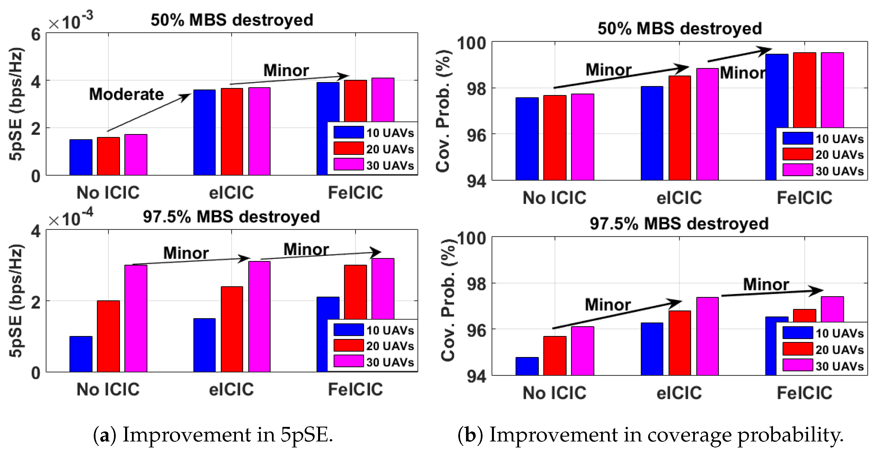
Figure 10.
Performance comparison when GUEs are distributed using MCP and UABS deployed on a fixed hexagonal grid.
Figure 11.
Peak 5pSE performance of the wireless network; when GUEs are distributed using TCP, UABS deployed on a fixed hexagonal grid, and for different ICIC techniques. (a) NIM Peak 5pSE vs. CRE. (b) eICIC Peak 5pSE vs. CRE. (c) FeICIC Peak 5pSE vs. CRE.
Figure 12.
Peak coverage performance of the wireless network; when GUEs are distributed using TCP, UABS deployed on a fixed hexagonal grid, and for different ICIC techniques. (a) NIM Coverage probability vs. CRE. (b) eICIC Coverage probability vs. CRE. (c) FeICIC Coverage probability vs. CRE.
Figure 13.
Performance comparison when GUEs are distributed using TCP and UABS deployed on a fixed hexagonal grid.
Table 1.
Literature review on whether clustered users were considered and type of distributions used for modeling the user clusters, optimization techniques used, and the optimization goals of the system model.
| Ref. | Cluster | User Distribution | Optimization Techniques | Optimization Goals |
|---|
| [30] | ✗ | ✗ | Swarm intelligence algorithms | resource scheduling, parameter optimization |
| [31] | ✗ | ✗ | Fuzzy C-means | resources optimization, path planning |
| [29] | ✗ | Equitably & randomly | Deep learning | interference coordination |
| [23] | ✗ | Randomly | Reinforcement learning | network coverage, optimal UAV placement |
| [21] | ✗ | Uniformly | Numerical | coverage, interference coordination |
| [5] | ✗ | Poisson point process (PPP) | Brute-Force, Genetic Algorithm | spectral efficiency, energy efficiency, interference coordination |
| [4] | ✗ | PPP | Brute-Force, eHSGA, Genetic Algorithm | spectral efficiency, energy efficiency, interference coordination |
| [32] | ✗ | PPP | Brute-Force, Genetic approach | spectral efficiency, coverage |
| [17] | ✗ | PPP | Q-learning, Deep Q-learning, Brute-force, Sequential algorithm | spectral efficiency, energy efficiency, interference coordination |
| [20] | ✓ | Fast K-means | Numerical | power optimization, resource allocation |
| [15] | ✓ | Poisson cluster process (PCP) | Stochastic geometry | coverage probability and downlink analysis |
| [33] | ✓ | TCP | Closed-form bounds | CDF of the nearest neighbor
and contact distance distributions of clusters |
| [34] | ✓ | MCP | Closed-form bounds | CDF of the nearest neighbor
and contact distance distributions of clusters |
| [35] | ✓ | PCP | Stochastic geometry to find correlation
between base-station cell locations | resource block management, coverage probability, throughput |
| [36] | ✓ | PPP, PCP | Geometry-based analysis | downlink coverage probability, interference coordination |
| Our Work | ✓ | TCP and MCP | Brute-Force | spectral efficiency, energy efficiency, interference coordination |
Table 2.
Notations and symbols used in the system model.
| Symbol | Description |
|---|
| Locations of MBS and UE. |
| , | Distribution intensities of the MBS and UE nodes |
| Maximum transmit power of MBS and UABS |
| Transmitter antenna’s 3DBF element of antennas for all base stations |
| F | Account for Nakagami fading |
| , | Respective path loss from MBS and UABS in dB |
| Carrier frequency in PSC band 14 |
| Altitude of the base station in Okumura–Hata model |
| Altitude of MBS and UABS |
| Altitude of a UE in Okumura–Hata model |
| UE distance from MOI and UOI |
| RSRP from MOI |
| RSRP from UOI |
| Aggregate interference at GUE from all base stations, except MOI/UOI |
| , | SIR from MOI and UOI in USF subframes |
| , | SIR from MOI and UOI in CSF subframes |
| MBS Power reduction factor during CSF transmission |
| Duty cycle for USF transmission |
| Cell range expansion bias |
| Scheduling threshold for MUE and UUE |
| Number of USF-MUEs and CSF-MUEs |
| Number of USF-UUEs and CSF-UUEs |
| Aggregate SEs for USF-MUEs and CSF-MUEs |
| Aggregate SEs for USF-UUEs and CSF-UUEs |
| Fixed hexagonal locations of deployed UABS |
| Matrix representation of ICIC parameters for MBSs |
| Matrix representation of ICIC parameters for UABSs |
| Radius of the Matern Cluster Process |
| Simulation area |
Table 3.
Shannon capacity definitions in terms of SIR and RSRP for USF/CSF radio frames.
| SIR Ratio | Shannon Capacity of USF/CSF Radio Frames |
|---|
| |
| |
| |
| |
Table 4.
Boundary values and the step size of each parameter to be optimized within the search space.
| Search Parameter | Parameter Range | Search Space Size |
|---|
| 0, , , … 1 | |
| 0, , , … 1 | |
| , + , + … | |
| , + , + … | |
| 0, , , … | |
| X coordinate of UABS | , | |
| Y coordinate of UABS | , | |
Table 5.
System parameters and simulation values considered.
| Parameter | Value |
|---|
| |
| , | 4 and 100 per km |
| 10, 20, 30 |
| 46 and 30 dBm |
| 36 and 120 m |
| 1.5 m |
| 763 MHz for downlink |
| 0 to 1 |
| 0 to 100% |
| 20 dB to 40 dB |
| dB to 5 dB |
| 0 dB to 12 dB |
Table 6.
Coverage probability peak value observations in % and when GUEs are distributed using TCP distribution.
| Brute Force Algorithm |
|---|
| | TCP Distribution |
| MBSs destroyed | 50% | 97.5% |
| No UABSs | 10 | 20 | 30 | 10 | 20 | 30 |
| NIM | 97.6870 | 97.7613 | 97.8160 | 95.1673 | 95.3484 | 96.4353 |
| eICIC | 99.4927 | 99.6142 | 99.7019 | 98.8974 | 99.1949 | 99.3506 |
| FeICIC | 99.9231 | 99.9541 | 99.9544 | 99.8530 | 99.9140 | 99.9310 |
Table 7.
Coverage probability peak value observations in % and when GUEs are distributed using MCP distribution.
| Brute Force Algorithm |
|---|
| | MCP Distribution |
| MBSs destroyed | 50% | 97.5% |
| No UABSs | 10 | 20 | 30 | 10 | 20 | 30 |
| NIM | 97.5664 | 97.6774 | 97.7281 | 94.7658 | 95.6932 | 96.1169 |
| eICIC | 98.0655 | 98.5168 | 98.8411 | 96.2666 | 96.7794 | 97.3837 |
| FeICIC | 99.4767 | 99.5146 | 99.5168 | 96.5326 | 96.8583 | 97.3923 |
Table 8.
5pSE peak value observations in bps/kHz and when GUEs are distributed using MCP distribution.
| Brute Force Algorithm |
|---|
| | MCP Distribution |
| MBSs destroyed | 50% | 97.5% |
| No UABSs | 10 | 20 | 30 | 10 | 20 | 30 |
| NIM | 0.0095 | 0.0097 | 0.0104 | 0.0001 | 0.0002 | 0.0003 |
| eICIC | 0.0116 | 0.0125 | 0.0134 | 0.0005 | 0.0010 | 0.0014 |
| FeICIC | 0.0149 | 0.0154 | 0.0165 | 0.0006 | 0.0013 | 0.0018 |
Table 9.
5pSE peak value observations in bps/kHz and when GUEs are distributed using TCP distribution.
| Brute Force Algorithm |
|---|
| | TCP Distribution |
| MBSs destroyed | 50% | 97.5% |
| No UABSs | 10 | 20 | 30 | 10 | 20 | 30 |
| NIM | 0.0015 | 0.0016 | 0.0017 | 0.0001 | 0.0002 | 0.0003 |
| eICIC | 0.0036 | 0.00365 | 0.0037 | 0.00015 | 0.00024 | 0.00031 |
| FeICIC | 0.0039 | 0.0040 | 0.0041 | 0.00021 | 0.00030 | 0.00032 |


