Modelling the Acoustic Propagation in a Test Section of a Cavitation Tunnel: Scattering Issues of the Acoustic Source

Abstract

The prediction of the underwater-radiated noise for a vessel is classically performed at a model scale and extrapolated by semi-empirical laws. The accuracy of such a method depends on many parameters. Among them, the acoustic propagation model used to estimate the noise measured at a model scale is important. The present study focuses on the impact of the presence of a source in the transverse plane. The scattering effect, often neglected in many studies, is here investigated. Applying different methods for computation, we perform several simulations of the acoustic pressure field to show the influence of the scattered field. We finally discuss the results and draw some conclusions about the scattering effect in our experimental configuration.

1. Introduction

Improving our understanding of underwater-radiated noise induced by a propeller is a global aim, not only for military reasons but also because of its impact on marine fauna. The operational requirements for naval and research vessels have recently observed an increasing demand for quieter ships, either to comply with the ship’s operational requirements or to minimise the influence of shipping noise on marine life. Even if the help of computational fluid dynamics (CFD) is an emerging way to predict the noise level emitted by a boat [1], experimental approaches with scaled model inside a cavitation model are still preferred nowadays [2], due to the repeatability and experience of the institutes. Other experimental facilities (like a depressurised tank [3]) deal with the same goals; however, most of institutes are performing experimental campaigns within cavitation tunnels. Many parameters have to be controlled to ensure an accurate measurement in such a facility. The different reviews we found in the literature dealing with a comparison between model-scale and full-scale estimates show that large discrepancies could be observed [4,5]. Numerical methods developed recently [6,7,8] are sometimes useful to understand or estimate the different features (magnitudes, position, and directivity) of the acoustic sources we find in the water flow around a model. Nevertheless, the experiments are still chosen to predict the noise on a full scale.

Proceeding with this method, the knowledge of acoustic propagation features remains one of the key points to ensure the reliability and accuracy of the global method. The test section of a cavitation tunnel could be compared to a corridor. Over several decades, different experiments have been performed inside ducts in air or water, with or without flow [9,10,11], with the aim to decompose the acoustic field into several propagative modes or to take into account the flow for acoustic propagation in square ducts [12]. Numerically, some developments have been developed recently [13], always with the goal of estimating the underwater-radiated noise with the best accuracy. The development of arrays of sensors has been set up [14] to enhance the signal-to-noise ratios that also allow for localizing the sources, for example. The sensor arrays could also be used to demodulate the acoustic field [15] and express the propagation inside the duct using the modal theory. Indeed, the acoustic propagation in the duct is widely studied around the world due to the numerous applications it covers. Among all these topics, the particular case of the underwater acoustic propagation in a cavitation tunnel is studied here with a focus on scattering effects due to the presence of a source.

The acoustic field in these facilities is of major importance when they are used to predict the underwater-radiated noise generated by a vessel equipped with its propulsor, for example. To estimate the future underwater noise level of a propeller, a raw measurement is performed in the test section. A correction step is then applied to these measurements to obtain (as much as possible) the acoustic power of the source. The measurements obtained at this model scale are then processed and scaled to the scale of the future boat. This estimate is even now subjected to large uncertainties due to many parameters that are not perfectly known or not taken into account [5,16]. The acoustic field that exists in a test section is fully different from the one at sea. These features need to be known and corrected properly to ensure the accuracy of the final estimate. We focus on the case of a cavitation tunnel test section. Figure 1 depicts a classical set up for such measurements.

In the test section, we introduce a model scale of the ship. The acoustic measurement is then performed thanks to hydrophone sensors. They could be flush-mounted on the walls of the test section or installed in the flow with struts, as depicted by the schematic drawing in Figure 1. The raw data obtained in such a configuration have to be processed in order to:

• Subtract the background noise of the facility when this noise could not be neglected;
• Represent the noise radiated by the model and not the facility;
• Represent, not the acoustic pressure at the position of the sensor, but the acoustic power radiated.

The knowledge of the acoustic source(s) positions is consequently one of the most important features. The use of the different institutes is to measure the distance between the source location and the hydrophones, and to correct the measurement by this distance in order to standardise the spectrum. This is only possible if the exact locations of the sources are known, which is not really the case: the sources of noise are located generally close to the propeller but their locations during a test are obviously moving and are not accurately known. Another approach consists in measuring the transfer functions between a standardised source and each sensor. This solution allows for taking into account main features of the facility (distance standardization, reverberation, reflections, etc.); however, it is required to insert the reference source at the exact location of the noise source. For the same reasons as the first method, it is not easy to set up, and a large part of the inaccuracy could be attributed to this distance approximation. Recently, Tani [17] or Boucheron [16] studied the diffuse field and the way to improve the measurement using transfer functions by, for example, averaging several transfer function measurements. The latter avoids the presence of high peaks that could be visible in a lonely transfer function. To measure a transfer function, the use of a dedicated device to generate a controlled signal in the test section is required. The size of this acoustic source is not taken into account in the method because it is considered as an acoustic monopole.

To improve the estimate, especially in the low frequencies’ domain, a solution for the acoustic propagation is to use the modal theory to describe the whole acoustic field. The image source theory uses different point sources to describe the whole field with different models of waves (plane waves, spherical waves, etc.). These models are used in the literature in the test section considering that the source could be modelled by a point (a monopole). This theory has been developed for room acoustic applications [18,19], but could also be used efficiently in duct acoustics, as has been conducted previously in water, for example, in [20]. A particularity of the devices used to generate acoustic waves in a water tunnel is the main size that could not be considered as a singular point. The result of a “large” dimension of an object in the acoustic field is a scattered field. This field could be computed but it requires a high power of calculus and time due to its complexity. This is why most of the studies are neglecting this field which is not the most important one (it is a field generated as a second-order field because it is the consequence of the incoming wave and an object). The present study is dedicated to provide an insight of the cases for which it could be considered reasonable to neglect this field and the cases for which this field has to be computed to reach the provided accuracy of the acoustic field. The different sources widely used in practice for acoustic tests have mainly two different shapes. The most used source is very similar to a sphere (the only difference is the cable which links the source to the amplifier). For low frequencies, another kind of source is used. The shape of such sources is generally a cylinder in which a piston is moving to generate the acoustic wave. Consequently, we have decided to investigate these two shapes for the scattered field.

The objectives of the study are then to assess the scattering effects in the case of spherical or cylindrical shapes that are encountered in the calibration process used to predict the underwater-radiated noise of a vessel. The next section presents, as evoked previously, the modal propagation in the duct, the image sources’ method, and the scattering theories for two geometries: the sphere and the cylinder. The third section will present the approach adopted here for simulations and computations. Then, we present and analyse the results obtained by these simulations. A discussion about the consequences of the simulations performed in a water tunnel for acoustic applications is then developed. Finally, we outline the main conclusions of this study.

2. Acoustic Theories

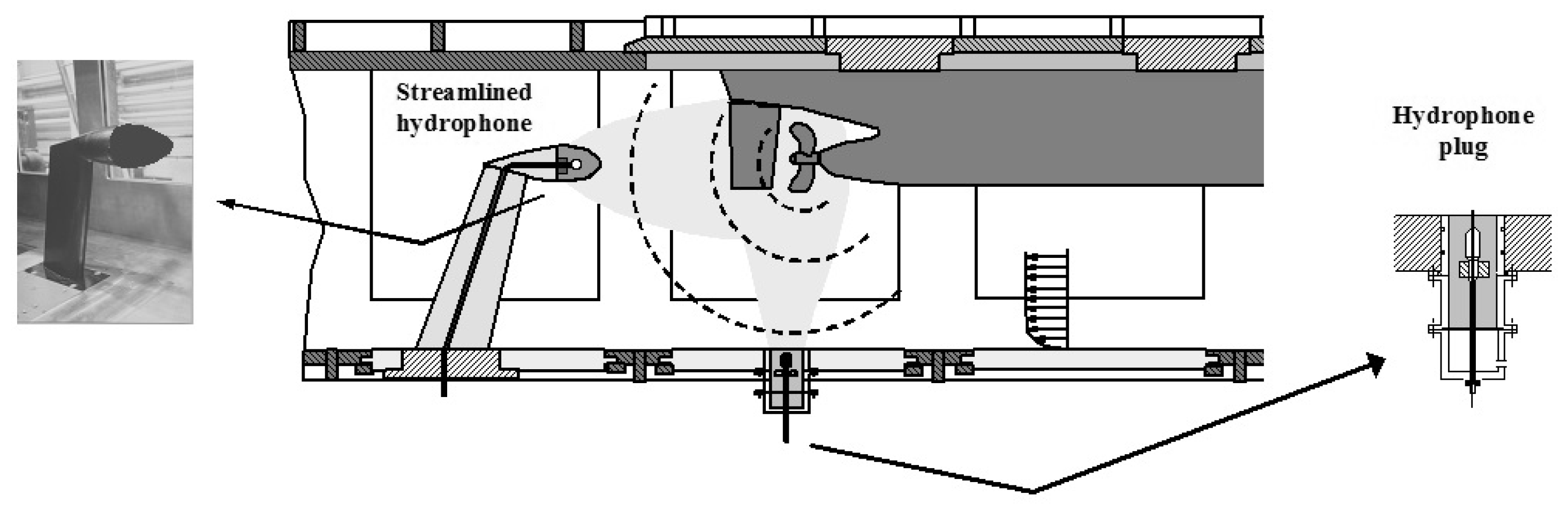
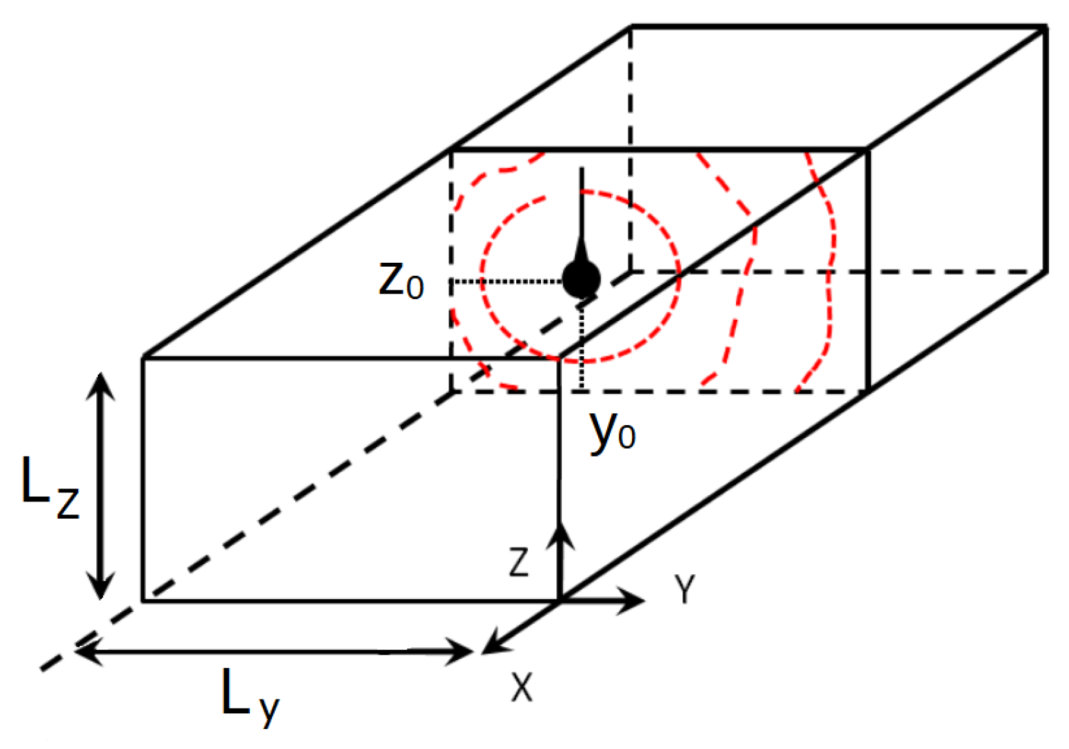
2.1. Modal Propagation in Duct

2.1.1. General Equations

The acoustic field inside a duct could be described by the modal propagation theory. In a perfect rectangular duct, the solution of the Helmholtz equation that describes the acoustic propagation could be expressed as a superposition of several modes according to [21,22,23]. This duct shape has been chosen because the shape of the test-section of most of the cavitation tunnels is rectangular. All of the theory could be adapted to the circular shape with the help of Bessel functions which modify the modal shape functions ${\psi }_{mn}(y,z)$, see [21] for an example. The acoustic pressure p inside the duct can be expressed as

$${\displaystyle p(x,y,z,t)=\sum _{m,n}{\Psi }_{mn}(y,z)\left[A_{mn}{e}^{\mathrm{j}{k}_{x,mn}x}+B_{mn}{e}^{-\mathrm{j}{k}_{x,mn}x}\right]\times e^{\mathrm{j}\omega t},}$$

(1)

$\omega$ being the angular frequency, $\mathrm{j}=\sqrt{-1}$, $k=\omega /c_0$ is the wavenumber and $c_0$ is the celerity in water. Here, $k_{x,mn}$ is the axial wavenumber associated with the mode (m, n). m (respectively, n) is the mode number on the y-dimension (respectively, z-dimension). The coefficients $A_{mn}$ and $B_{mn}$ are the complex magnitudes associated with the upstream (respectively, downstream) direction of the propagation. If hard-wall conditions are considered, the wave equation leads to modal shapes ${\Psi }_{mn}$ expressed by

$${\Psi }_{mn}(y,z)=cos\left({\displaystyle \frac{m\pi y}{L_y}}\right)\times cos\left({\displaystyle \frac{n\pi z}{L_z}}\right).$$

(2)

$L_y$ and $L_z$ are the different lengths of the section (for a square section, $L_y=L_z$). Introducing these equations in the general Helmholtz equation, we obtain the classical dispersion equation for the rectangular duct

$$k_{x,mn}=\sqrt{{\left({\displaystyle \frac{\omega }{c_0}}\right)}^2-{\left({\displaystyle \frac{m\pi }{L_y}}\right)}^2-{\left({\displaystyle \frac{n\pi }{L_z}}\right)}^2}.$$

(3)

The limiting value ($k_{x,mn}=0$) determines the cut-off frequency $f_{mn}^c$, given by

$$f_{mn}^c={\displaystyle \frac{c_0}{2}}\sqrt{{\left({\displaystyle \frac{m}{L_y}}\right)}^2+{\left({\displaystyle \frac{n}{L_z}}\right)}^2}.$$

(4)

For a given mode (m, n), only frequencies higher than $f_{mn}^c$ can propagate. Other modes (denoted by a wavenumber that is purely imaginary) are called “evanescent” and no acoustic energy is propagated within this mode.

2.1.2. Modal Magnitudes $A_{mn}$

Assume that a source is located in the test section in accordance with Figure 2.

The energy radiated by this source will propagate in the test section following the different modal shapes ${\Psi }_{mn}$. The different complex magnitudes of the modes are fully determined by the transverse position of the source in the test section ($y_0$, $z_0$) by

$$A_{mn}={\displaystyle \frac{\mathrm{j}}{2S{k}_{mn}}}{\displaystyle \frac{{\Psi }_{mn}(y_0,z_0)}{{\Lambda }_{mn}}},$$

(5)

with the different parameters expressed as

$${\Lambda }_{mn}=N_{ym}\times N_{zn},N_{ym}={\displaystyle \frac{1}{{ϵ}_m}},N_{zn}={\displaystyle \frac{1}{{ϵ}_n}},$$

(6)

with ${ϵ}_0=1$, ${ϵ}_n=2$ for $n\ge 1$ and $S=L_y\times L_z$. The computation of the acoustic pressure field can be conducted in any location in space inside the test section thanks to the knowledge of the positions of the sources. It has to be noticed that acoustic sources are calibrated; for example, the sensitivity measured corresponds to the one of the monopole. Thus, the acoustic power of a given source is sufficient to estimate the acoustic pressure field in the domain.

Another theory could be used also to predict the whole acoustic field close to the source: the image source theory. It is shortly described in the next paragraph.

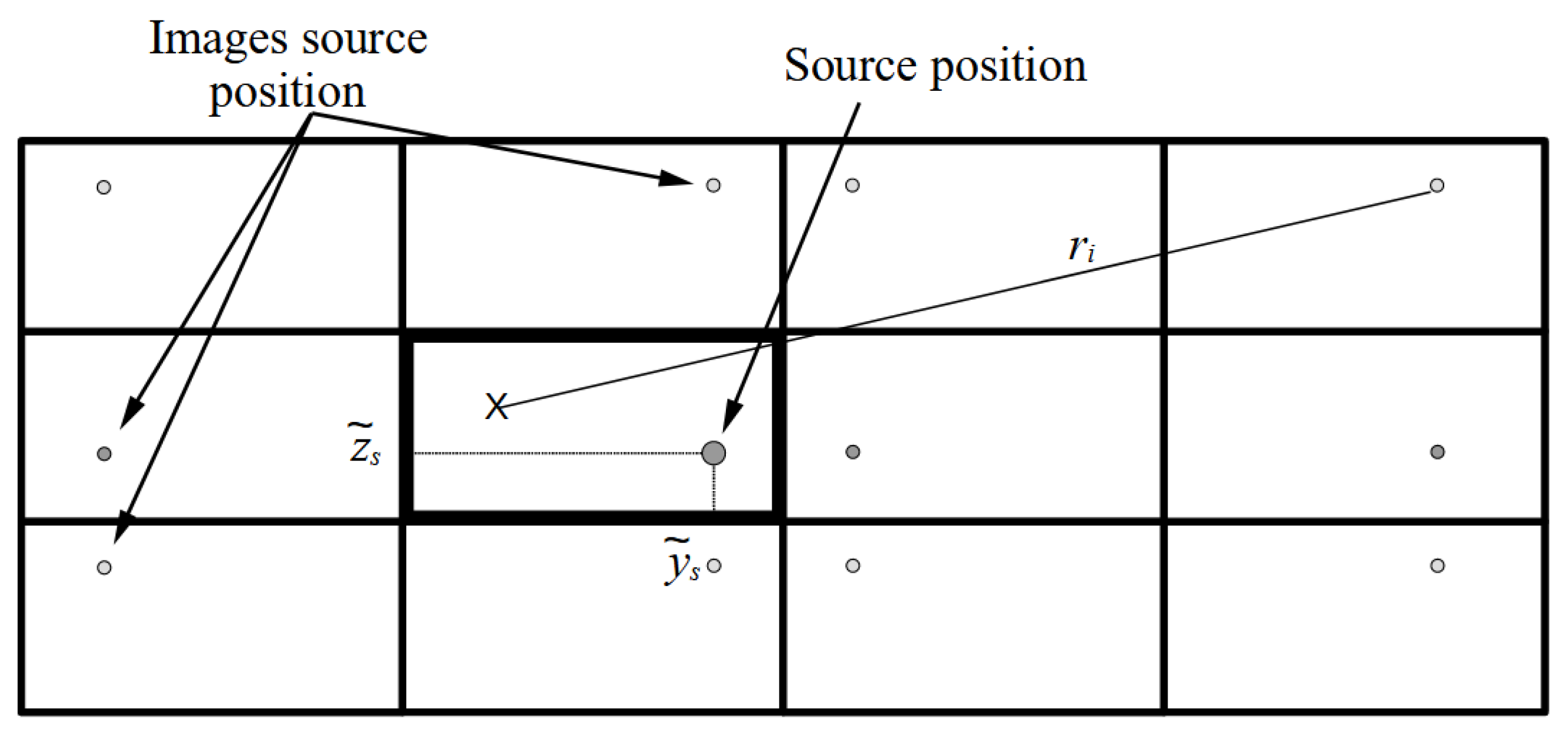
2.2. Image Sources Theory

The whole acoustic field generated by a source inside a test section of a cavitation tunnel could be computed by the image theory [22]. Indeed, this environment is similar to a room with walls for which this theory has been developed.

Figure 3 presents a schematic drawing that explains the principle of this method. The bold rectangle represents the transverse test section. The big grey circle is the real acoustic source (coordinates ($\widetilde{y_s}$, $\widetilde{z_s}$)) whereas the x depicts the receiver under consideration. Other grey dots depict the image source positions which could be calculated by simple geometrical laws by reflection. Consequently, the distance $r_i$ is the distance between the receiver and the ith image source. Thus, the methods consists of

• Computing the image sources locations from geometrical features, up to the order of $n_{\mathrm{I}}$,
• Considering that each source is a monopole;
• Computing the contribution of each image source in agreement with wall characteristics (reflection laws);
• Adding all the contributions to obtain the global acoustic field.

This theory is quite easy to set up from a simulation point of view. However, there remain several drawbacks. The most important image sources are the first-order sources, because they are close to the field of interest. The higher the order of the source, the less importance of this source. But, it is not easy to accurately determine the maximum order to be computed to assess a given accuracy: this could be tackled by driving a convergence study. Even if this kind of study takes time, it allows for the assessment of the order parameter $n_{\mathrm{I}}$. Moreover, the magnitude of each image source has to be weighted by the wall impedances to take into account the reflection on the walls. The values of the wall impedance are not easy to evaluate practically. The amplitude of an image source of order $n_{\mathrm{I}}$ is roughly proportional to this multiplicative coefficient at the power $n_{\mathrm{I}}$. Consequently, an error on this coefficient increases exponentially with the order of the source. Another important source of the error not taken into account in most of the studies using image source theory is the fact that the acoustic source, in practice, could not be considered as a point. After the first reflection of the wave from the wall, the wave encounters the source (similar to a sphere or a cylinder) and a scattering effect of this wave occurs.

The image theory uses a distribution of monopoles. The best way to express the acoustic pressure radiated by a monopole is using the spherical coordinates. The scattered field is also easier to express with these coordinates. However, the plane wave travelling in a 2D space (the field that we will simulate in our study) has to be written in this system of coordinates: this is conducted in the following paragraph for both cases (sphere and cylinder).

2.3. Model Expressed in Spherical Tools

With the aim of expressing the scattered field, here we recall the propagation theory with spherical tools (spherical coordinates and spherical functions). Here, we use the classical spherical coordinates (r, $\theta$, $\phi$). Firstly, the experimental configuration is assumed to be an acoustic source located at the origin of space ($r=0$). This assumption is important because it allows us to apply the monopole theory that mathematically simplifies the governing equations. Indeed, an acoustic monopole generates an acoustic pressure that is fully described by this simple equation (expressed in spherical coordinates $r,\theta ,\phi$):

$$p(r,\theta ,\phi ,t)=A{e}^{\mathrm{j}k(r-c_{0}t)},$$

(7)

with A being the amplitude of the wave. This simple equation is very useful because of its simplicity and its easiness to be computed in different situations. It could be noticed, for example, that there is no dependence on $\theta$ or $\phi$ for an ideal monopole.

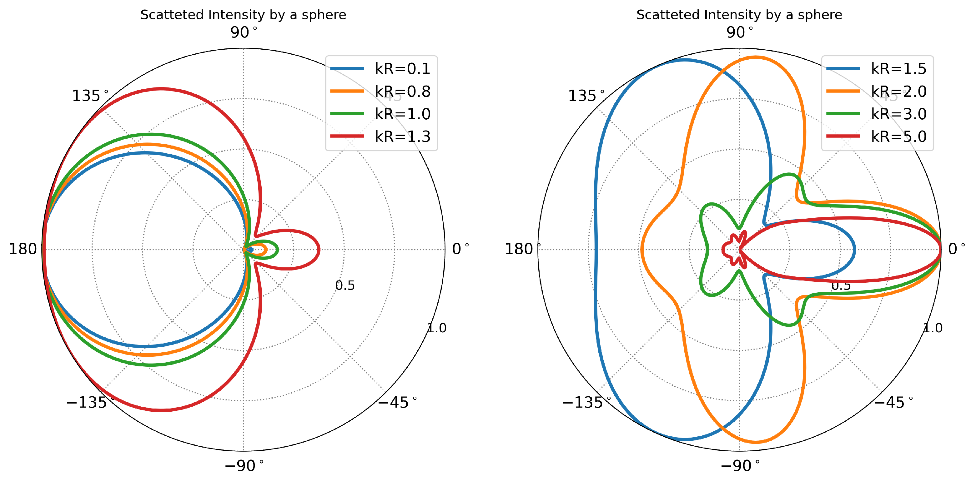
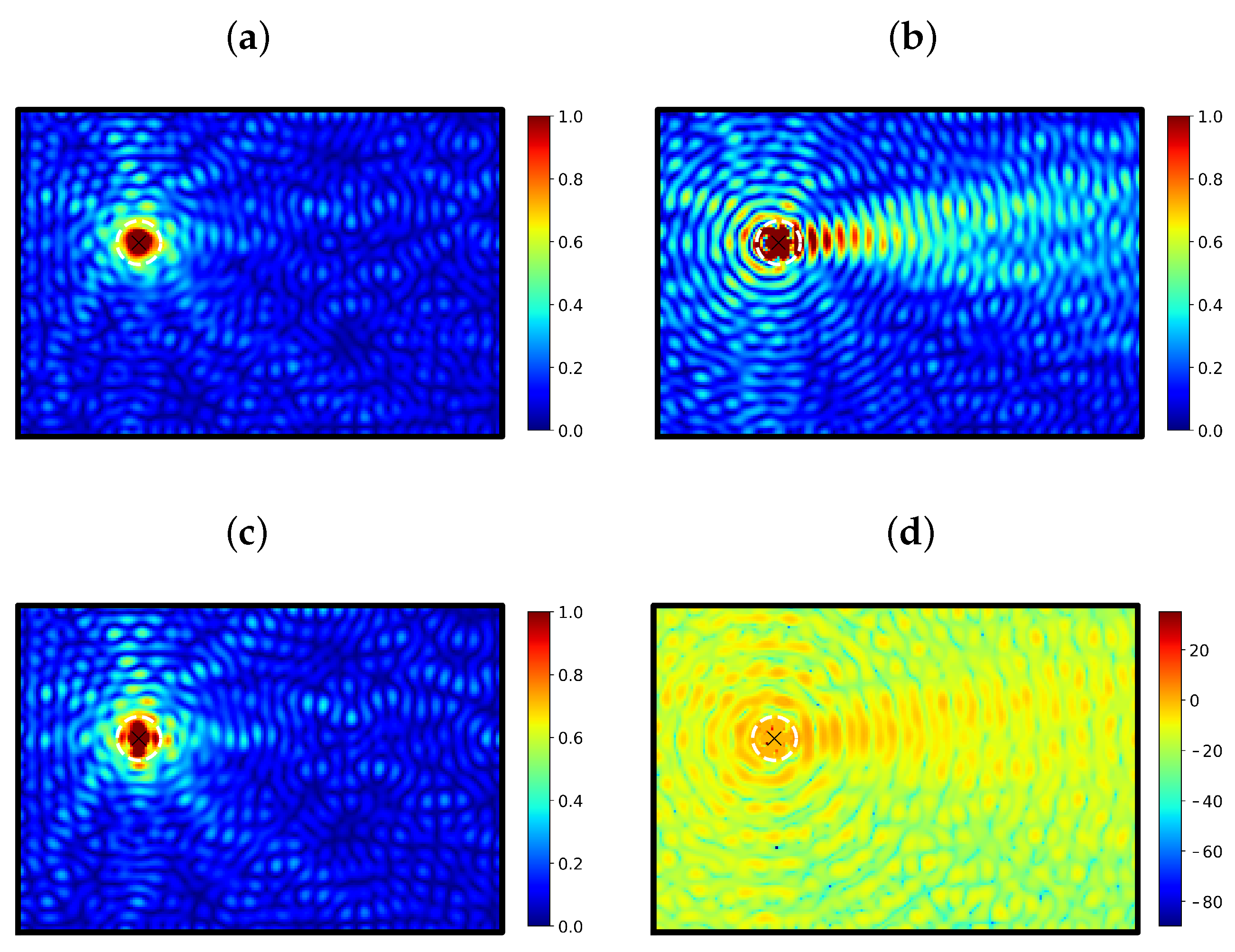
2.3.1. Scattering by a Sphere

In the spherical coordinate system, a plane wave travelling along a polar axis ($\theta =0$) could be described by

$${\displaystyle p_i(r,\theta ,\phi ,t)=A{e}^{\mathrm{j}k[rcos\left(\theta \right)-c_{0}t]}=A\sum _{m=0}^{\infty }(2m+1){\mathrm{j}}^m{\mathrm{P}}_{\mathrm{m}}\left(cos\left(\theta \right)\right){\mathit{j}}_{\mathit{m}}\left(kr\right)e^{-\mathrm{j}\omega t},}$$

(8)

with ${\mathrm{P}}_{\mathrm{m}}\left(x\right)$ being the Legendre function of order m and ${\mathit{j}}_{\mathit{m}}\left(x\right)$ being the spherical Bessel function of the first kind (see Morse and Ingard [21] and Abramovitz [24] for more information on these functions). If a sphere of the radius R is placed at $r=0$ (the origin of the coordinate system), the scattered wave could be expressed by [21]:

$${\displaystyle p_s(r,\theta ,\phi ,t)=-A\sum _{m=0}^{\infty }(2m+1){\mathrm{j}}^{m+1}{e}^{-\mathrm{j}{\delta }_m}sin\left({\delta }_m\right){\mathrm{P}}_{\mathrm{m}}\left(cos\left(\theta \right)\right)\left[{\mathit{h}}_{\mathit{m}}^{\left(\mathit{1}\right)}\left(kr\right)\right]e^{-\mathrm{j}\omega t},}$$

(9)

with ${\mathit{h}}_{\mathit{m}}^{\left(\mathit{1}\right)}\left(x\right)={\mathit{j}}_{\mathit{m}}\left(x\right)+\mathrm{j}{\mathit{n}}_{\mathit{m}}\left(x\right)$ being the first spherical Bessel function of the third kind (${\mathit{j}}_{\mathit{m}}\left(x\right)$ and ${\mathit{n}}_{\mathit{m}}\left(x\right)$ are the spherical Bessel functions of the first (respectively, second) kind). ${\delta }_m$ is the angle defined by the derived spherical Hankel function of the first kind (the first spherical Bessel functions of the third kind). To obtain this latter equation, we only used the impedance of the sphere material to compute the acoustic velocity at the interface. Solving the equation of velocity allows us to obtain the values of the magnitudes of each mode. It yields:

$${\left.{\displaystyle \frac{\partial {\mathit{h}}_{\mathit{m}}^{\left(\mathit{1}\right)}\left(z\right)}{\partial z}}\right]}_{z=kR}=\mathrm{j}{B}_m\left(z\right)\times e^{\mathrm{j}{\delta }_m\left(z\right)}{]}_{z=kR}$$

(10)

$B_m$ is the magnitude and ${\delta }_m$ is the phase. The computation of the scattered intensity by a plane wave could be conducted by:

$${\displaystyle I_s(r,\theta ,\phi ,t)\approx {\displaystyle \frac{I}{r^2{k}^2}}\sum _{m,n=0}^{\infty }(2m+1)(2n+1)sin\left({\delta }_m\right)sin\left({\delta }_n\right)cos({\delta }_m-{\delta }_n){\mathrm{P}}_{\mathrm{m}}\left(cos\left(\theta \right)\right){\mathrm{P}}_{\mathrm{n}}\left(cos\left(\theta \right)\right).}$$

(11)

The scattering pattern is highly dependent on the frequency. As an example, Figure 4 presents directivity patterns obtained with Equation (11) for different values of $kR$. This parameter could be associated to the frequency: with a given size of sphere R, then $kR=2\pi fR/c_0$ is proportional to the frequency.

It could be observed that for low frequencies (for $kR<1$), the presence of the sphere imposes back reflections with the most important magnitudes. Conversely, for higher frequencies ($kR=5$, for example), the main directivity lobe is oriented in the direction of the incident wave (travelling from the left to the right in our configuration).

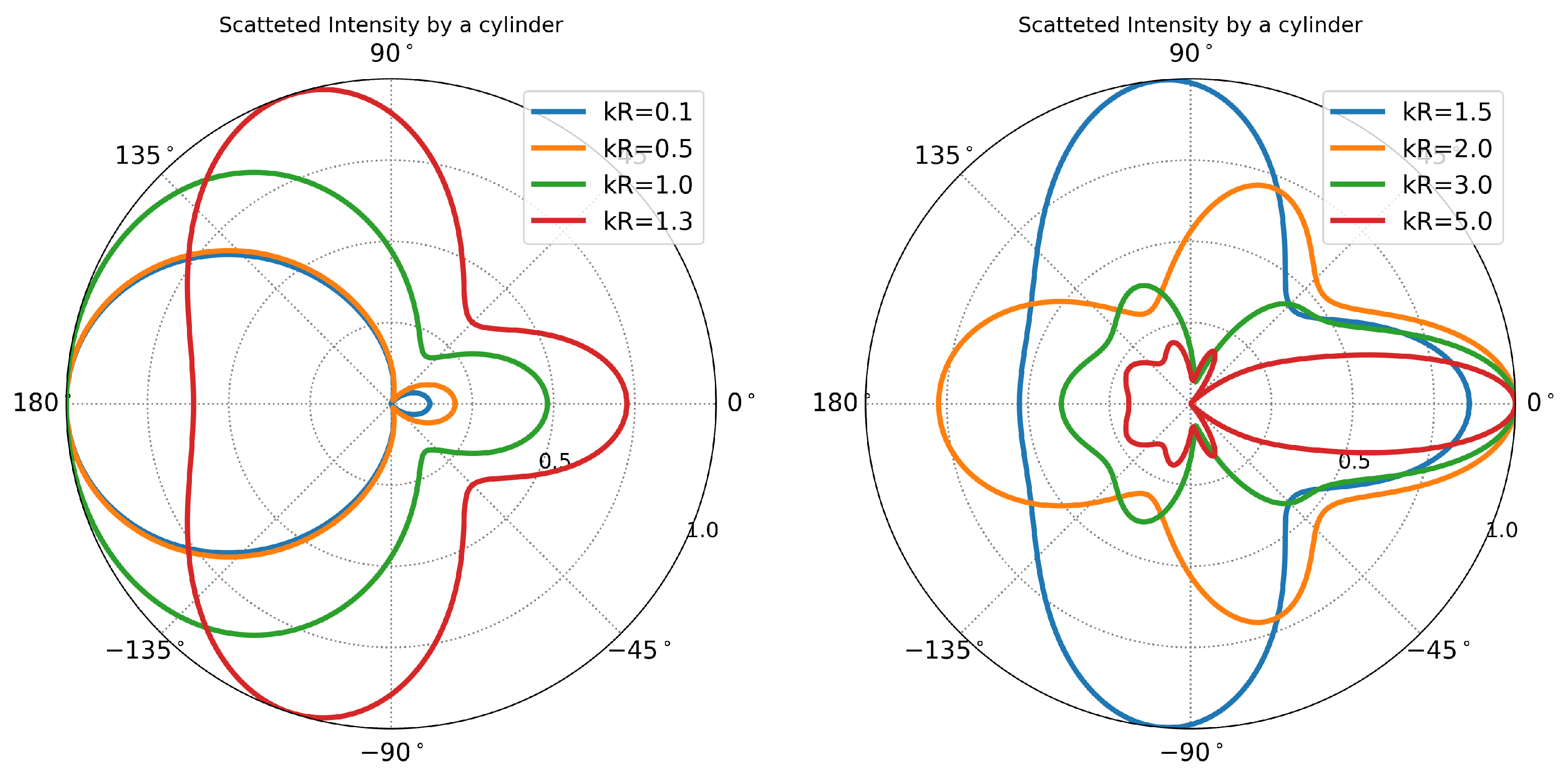
2.3.2. Scattering by a Cylinder

In this study, we investigate another classical case we can encounter in practice: the field scattered by a cylinder. The acoustic field scattered by a cylinder of radius R is given (in classical cylindrical coordinates (x, r, $\theta$) by:

$${\displaystyle p(x,r,\theta ,t)=\sum _{m=1}^{\infty }{A}_{m}cos\left(m\theta \right)\left[{\mathrm{J}}_{\mathrm{m}}\left(kr\right)+\mathrm{j}{\mathrm{N}}_{\mathrm{m}}\left(kr\right)\right]e^{-\mathrm{j}\omega t},}$$

(12)

with the magnitudes given by

$$A_m=-{ϵ}_m{P}_0{\mathrm{j}}^{m+1}{e}^{-\mathrm{j}{\gamma }_m}sin\left({\gamma }_m\right),$$

(13)

and angles expressed as

$$\begin{array}{ccc}\hfill tan\left({\gamma }_0\right)\hfill & =& \hfill -{\displaystyle \frac{{\mathrm{J}}_1\left(kR\right)}{{\mathrm{N}}_1\left(kR\right)}}\hfill \\ \hfill tan\left({\gamma }_m\right)\hfill & =& \hfill {\displaystyle \frac{{\mathrm{J}}_{\mathrm{m}-1}\left(kR\right)-{\mathrm{J}}_{\mathrm{m}+1}\left(kR\right)}{{\mathrm{N}}_{\mathrm{m}+1}\left(kR\right)-{\mathrm{N}}_{\mathrm{m}-1}\left(kR\right)}},\hfill \end{array}$$

(14)

with ${ϵ}_0=1$ and ${ϵ}_m=2$ for all $m>1$. The scattered intensity is then given by

$${\displaystyle I_s(r,\theta ,\phi ,t)\approx {\displaystyle \frac{I}{rk}}\sum _{m,n=0}^{\infty }{ϵ}_m{ϵ}_{n}sin\left({\gamma }_m\right)sin\left({\gamma }_n\right)cos({\gamma }_m-{\gamma }_n)cos\left(m\theta \right)cos\left(n\theta \right).}$$

(15)

We can observe the same behaviour as in the spherical case. For low frequencies (low $kR$), the back reflection is more important than the scattered wave in the direction of the incident wave. In return, for high frequencies, the direction of the most important magnitude of the scattered wave is the direction of the incident wave. We can observe some small differences by comparing the two Figure 4 and Figure 5 but the global behaviour is the same. This is normal because in a pure 2D test section, the cross-sections of a sphere and a cylinder with the same radius are the same.

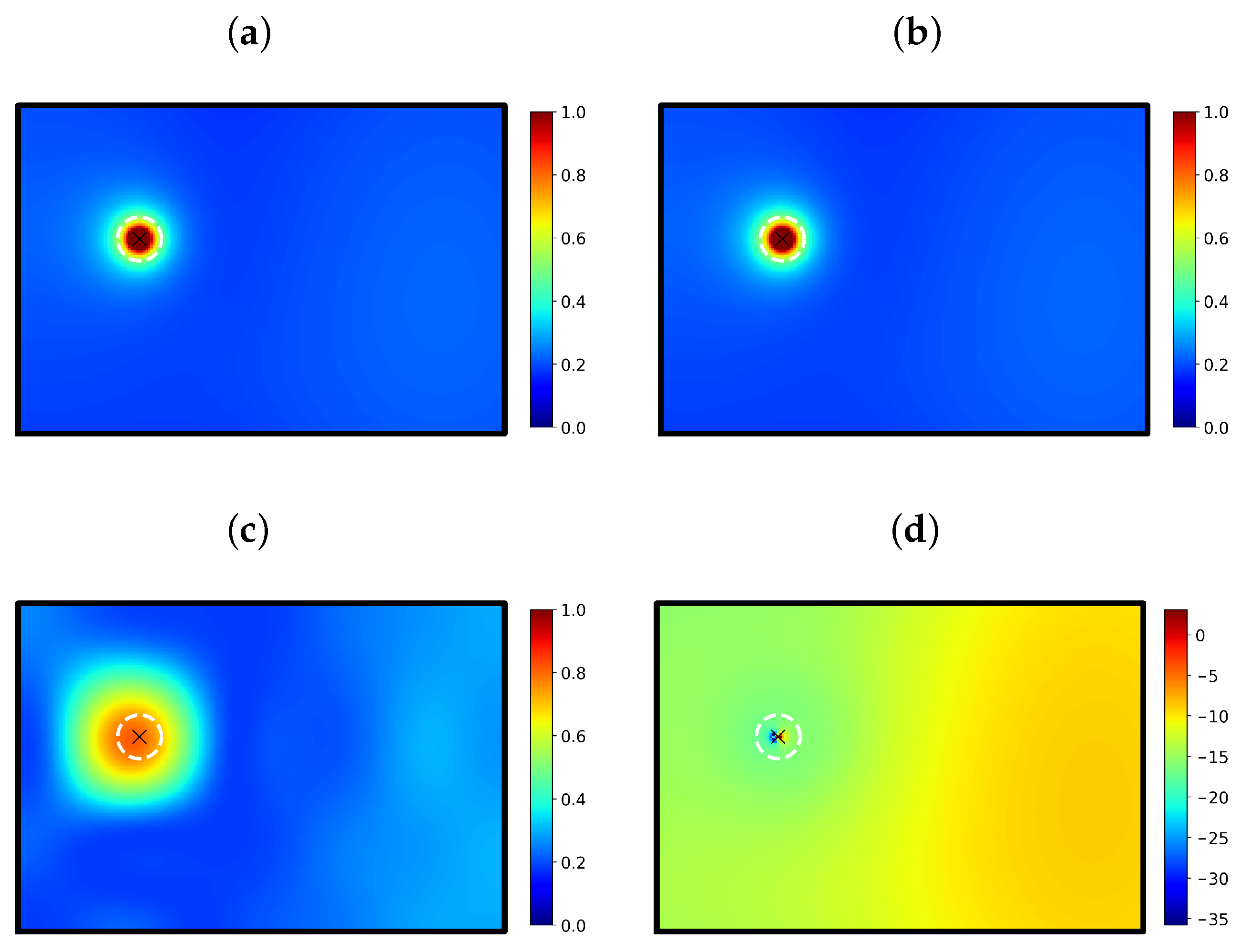
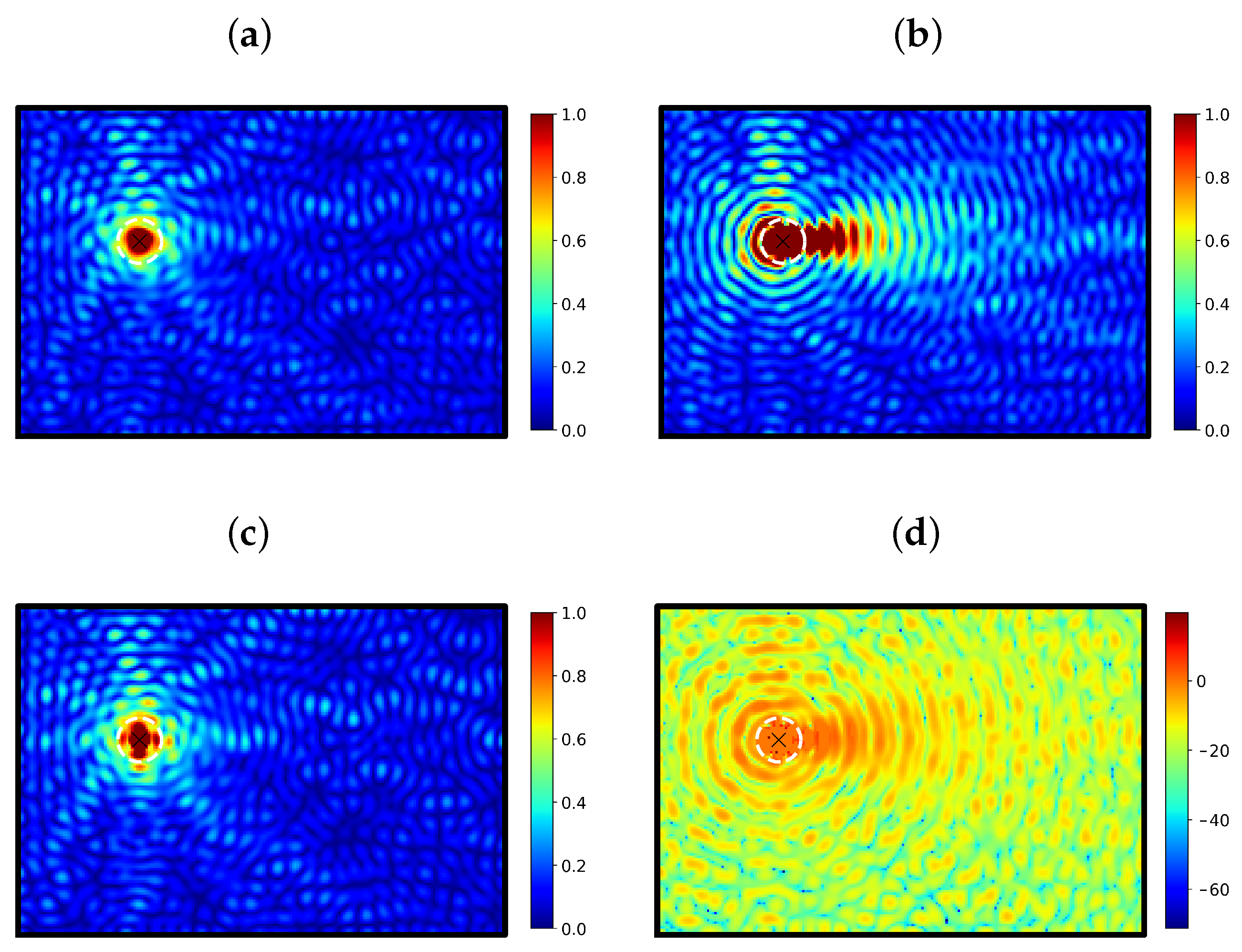
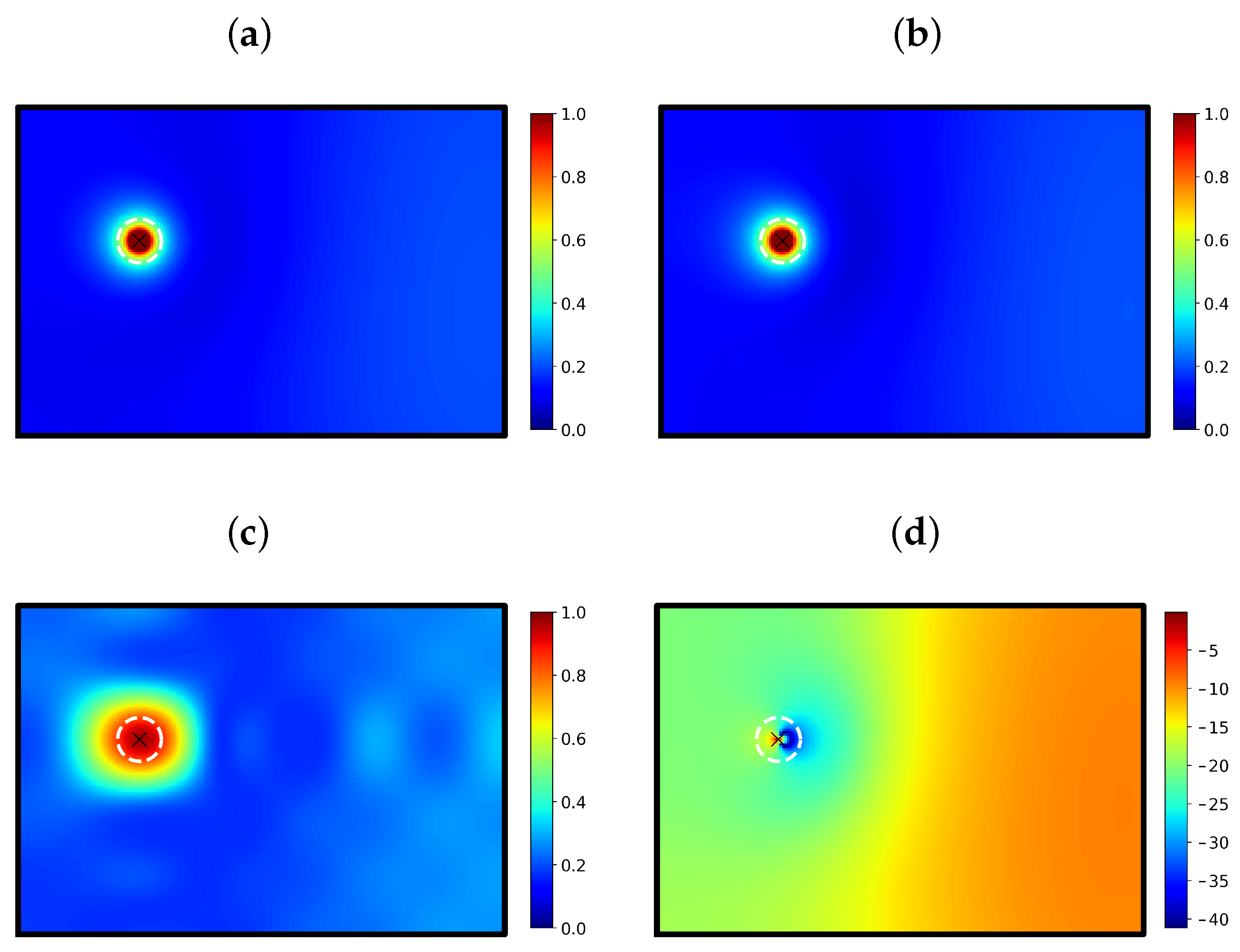
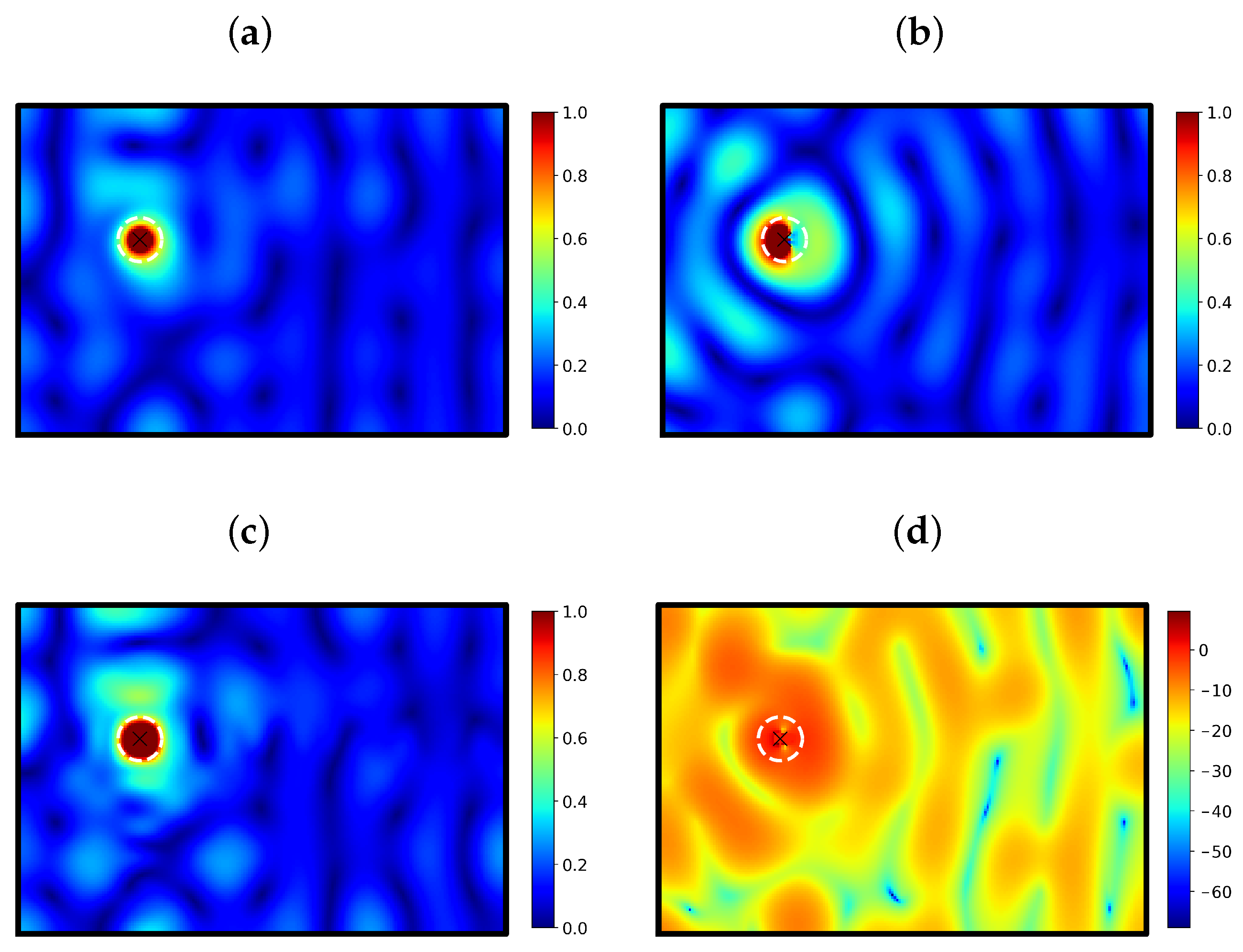
3. Results of Simulations

In this section, we present the different results obtained by the different computations. The principle is to compute the whole acoustic pressure field in the test section where is the source. This computation is conducted in three different ways: the first uses the classical image source theory (without taking into account the scattered field), the second is the same but taking into account the scattered field, and the third one is the computation with the modal theory. We focus on differences between these fields. For all simulation in a test section of a cavitation tunnel, we have fixed the impedance of the wall to $Z_W/Z_{\mathrm{water}}=30-1.0\mathrm{j}$. This value has been found to be the average values of the wall of our cavitation tunnel [15]. In order to be sure not to misinterpret the results, we first set up a short and simple study on the computations of the spherical Bessel functions. This is presented in the next section.

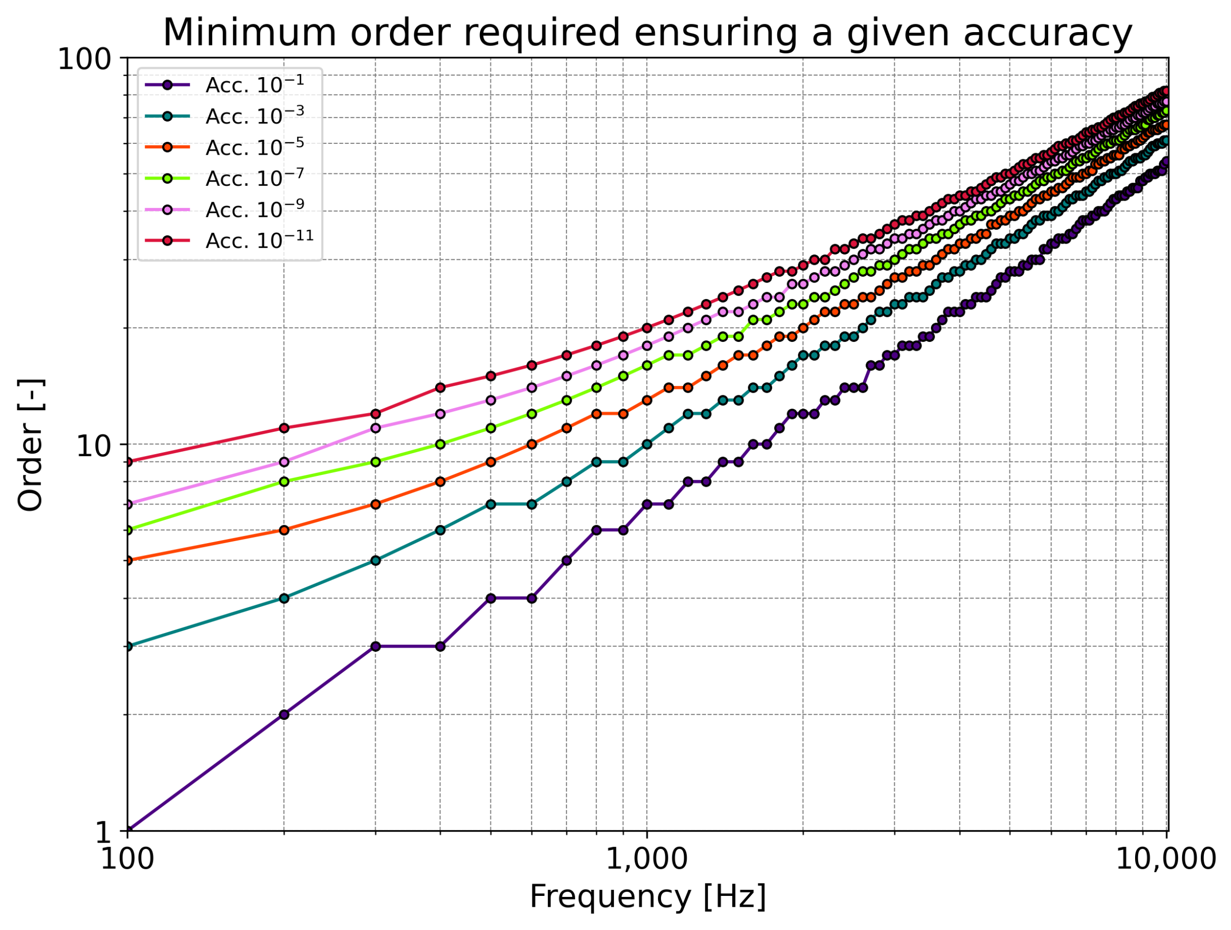
3.1. Assessment of the Accuracy for Spherical Bessel Functions’ Computation

The present study uses the spherical Bessel functions of the first, second and third kind ${\mathit{j}}_{\mathit{m}}\left(x\right)$, ${\mathit{n}}_{\mathit{m}}\left(x\right)$ and ${\mathit{h}}_{\mathit{m}}^{\left(\mathit{1}\right)}\left(x\right)$. For a plane wave, the whole acoustic pressure field could be computed with only the exponential function, see Equation (8). The equivalence by the infinity summation, even if it is mathematically exact, is not possible in practice. A maximal order has to be defined. This is conducted in combination with the researched accuracy. Fortunately, because we have the equivalence between an exact solution (that is easy to compute) and this summation, we can compute the two fields: the exact one $p_{ex}(r,\theta ,\phi ,t)$ and a truncated one $p_{tr}(r,\theta ,\phi ,t)$, as

$$p_{ex}(r,\theta ,\phi ,t)=A{e}^{\mathrm{j}k[rcos\left(\theta \right)-c_{0}t]},$$

(16)

$${\displaystyle p_{tr}(r,\theta ,\phi ,t)=A\sum _{m=0}^{\infty }(2m+1){\mathrm{j}}^m{\mathrm{P}}_{\mathrm{m}}\left(cos\left(\theta \right)\right){\mathit{j}}_{\mathit{m}}\left(kr\right)e^{-\mathrm{j}\omega t}.}$$

(17)

By computing the difference between the two fields and taking the maximum absolute value of this difference, we can obtain an estimate of the accuracy of the computation with the infinite summation. Figure 6 presents such a computation.

The most important error could be observed in the corners of the domain. This is expected because the geometrical origin is located at the centre of the domain and the most important values will be found for the larger $kr$.

Figure 7 presents the results in our configuration. The minimum order of the spherical Bessel functions is represented against the frequency. Six curves are plotted, representing six different accuracies. It could be observed that the behaviour of each curve is monotonic and quasi-linear. The higher the required accuracy, the higher the number of modes. This allows us to easily to predict the required order of the summation for any computation.

In our case, the order is more or less linear with the frequency and with the power order of the accuracy. We can summarise the required order by the following equation, available only in our case ($R_{\max }=\sqrt{L_y^2+L_z^2}=\sqrt{2^2+1.{35}^2}=2.41$ m):

$$n\approx \left[0.700+1.277\times {log}_{10}\left({\displaystyle \frac{1}{A}}\right)\right]+\left[5.144+0.1768\times {log}_{10}\left({\displaystyle \frac{1}{A}}\right)\right]\times f$$

(18)

with f being the given frequency in kHz and A being the researched accuracy. We use this model to reach a given accuracy in the following computations.

3.2. Spherical Case

Thanks to the model for obtaining a given accuracy with spherical functions, it is possible to compute the whole acoustic field in a test section with a target accuracy. This has been conducted for different approaches. The first one comes from the image theory without a scattered effect, as applied in most of the studies. The second method uses image theory, taking into account the scattered field and computed with the method described above. The third case is the modal theory computation described in Section 2.1. Results for $kR=1.0$ are presented in Figure 8.

At the upper left, we present the whole acoustic field computed without the scattered field; in the upper right we present the same acoustic field with the scattered component. The result from the modal acoustic method is displayed at the bottom left of the figure. At the bottom right, we have computed the difference between the two acoustic fields and scale this difference in dB. Each acoustic field is standardised so that the maximum of the pressure in the whole field is set to 1 Pa to facilitate the comparison. The source position is drawn with a black X on each sub-figure. The size of the modelled source ($R=9$ cm) is represented by the white dashed line on each sub-figure. Consequently, the field inside the white circle is not to be analysed because it does not exist in reality.

We can observe that the three acoustic fields are rather close. A detailed analysis shows that small discrepancies exist and are located mainly close to the source. The difference field (bottom right of Figure 8) is helpful to locate the locations of the maximum difference. In this case, we can observe that the difference is about $-20$ dB over the whole field, except in the near field where the scattered field is more important. Figure 9 presents the same results for the case $kR=0.1$ (low frequencies).

The acoustic fields from image theory are very close (with and without the scattered field) but differences are clearly observed close to the source with the modal theory. A reason could be the fact that for very low frequencies, the axial wavenumbers are quickly decreasing with the order of the mode. As noticed in [20], the computation of modes close to the test section of the source is tricky and could present some bias at low frequencies. Hence, the reconstruction of the acoustic field could be biased when it is close to the source. Nevertheless, the difference is about $-10$ dB over the whole field. In this case of low frequencies (below the cut-on frequency of the test section), the scattered field has no influence (as it could be expected due to the large wavelength). The last case presented here in the spherical configuration is for higher frequencies ($kR=5.0$). Results are presented in the Figure 10.

We can firstly observe that the two theories provide very close results (Figure 10a) and (Figure 10c). The scattering field is more pronounced for this case at a high frequency. The difference (of around 0 dB, meaning that the orders of magnitude are the same) is no longer located close to the source but on the whole field. Moreover, the directivity of the source (that is the evolution of the energy radiated against the direction) is highly modified. We can observe some important energy lobes on the difference image (Figure 10d) which means directivity changes. Obviously, the extrapolation of experimental measurements using the propagation model of case (a), case (b), or case (c) will provide different results and could be at the origin of inaccuracy.

3.3. Cylindrical Case

In this section, we report the same computations as the spherical case but with the cylindrical scattered field in the place of the spherical one. The three case $kR=0.1$, $kR=1.0$ and $kR=5.0$ are displayed, respectively, in Figure 11, Figure 12 and Figure 13.

For the three values of $kR$ investigated in this study, the results are close to the same in the cylindrical case as well as the spherical one. For the low frequencies $kR=0.1$, the acoustic pressure fields are very similar (Figure 9 and Figure 11). As noticed above and in accordance with the literature on the scattering effect, it is expected that small objects have a scattered effect that could be neglected. This is what we have found here in our simulations for both cases. Some small differences could be observed between the two cases at $kR=1.0$. Even if the order of magnitude of the different fields (acoustic fields and difference fields) are the same, we can observe the difference between the spherical case and cylindrical one. The 3D effect which is involved between these two cases does not produce huge discrepancies on the acoustic pressure field for mid frequencies. Then, this result suggests that both models (sphere/cylinder) could be used to model the scattering effect for both configurations without generating low accuracy. The cylinder model, being more easy to compute, could be considered for use in this frequency domain for studies requiring a high amount of computation (which allows, consequently, us to reduce the time consumption).

For high frequencies ($kR=5.0$), the behaviour is different. Even if globally we can observe for both cases a difference of around 0 dB in Figure 13, the acoustic pressure fields are different. In particular, the results in directivity are different: this is a consequence of the 3D effect and the model of the scattering effect due to the geometry. Then, for high frequencies, the scattered field has to be computed with the appropriated model to take into account this effect. Performing this way, the acoustic pressure field could be modelled with a higher accuracy.

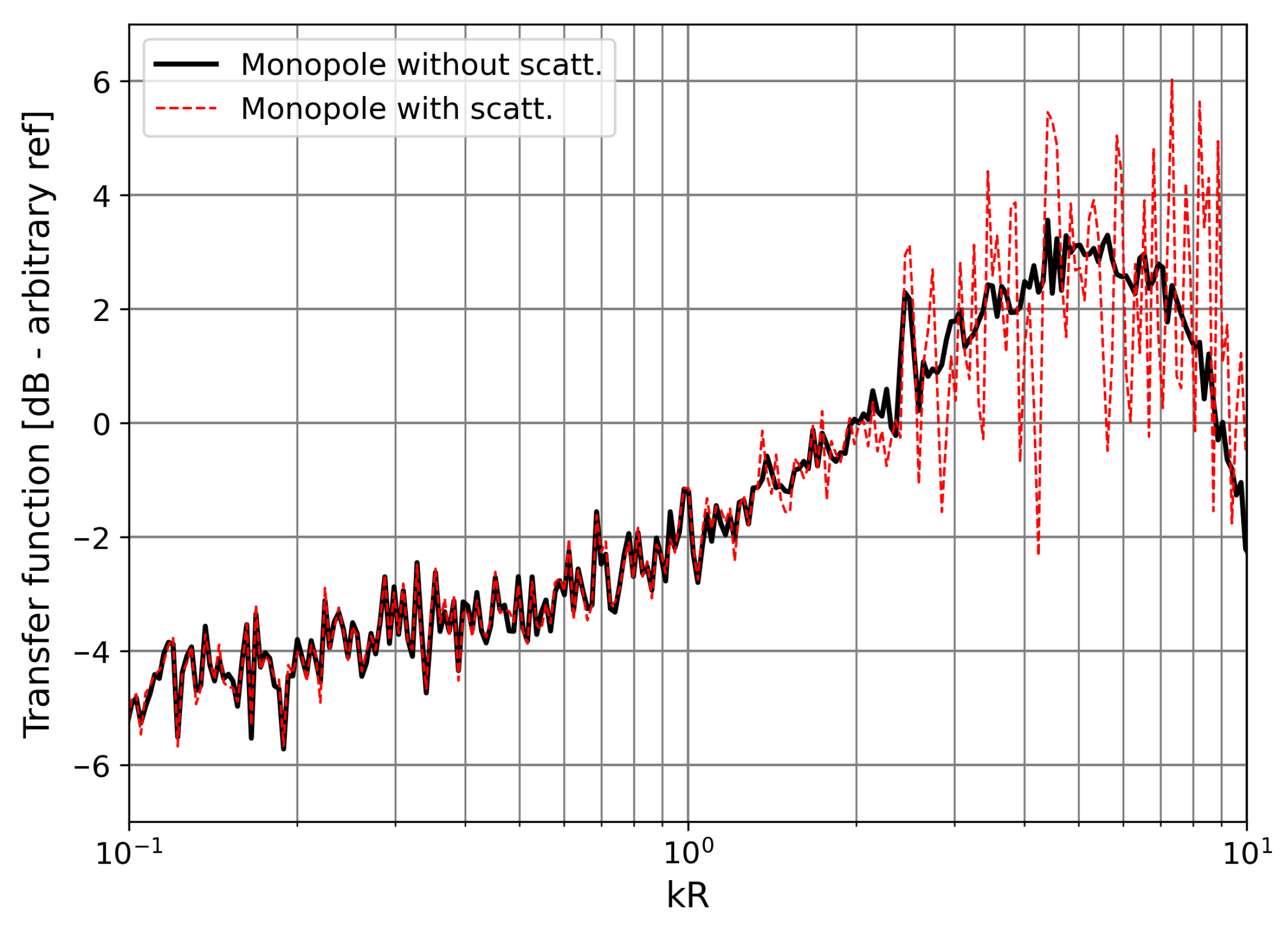
3.4. Consequences for Transfer Function Measurements

Finally, we present a last simulation of a transfer function measurement. We have chosen a noisy fictitious spectrum and send it to the acoustic source inside the test section. The position of this source is the same as the one used in the previous sections (see Figure 8). A hydrophone has been defined and flush-mounted on the vertical wall on the right. We consider the situation where a transfer function is measured (to further correct the raw measurements of the noise from a foil or a propeller in a flow). The correction is based on the fact that the calibration features of the source are well-known in a free field. Then, measuring the voltage provided to the source permits the knowledge of the acoustic pressure generated by the source at a given distance (generally 1 m) as long as the domain is a free-field one. Consequently, we have computed the spectrum measured by the hydrophone with and without taking into account the scattering effect. Results are shown in Figure 14.

Two curves are represented in this figure. The black one is the fictitious spectrum representing the classical case without the scattering effect. The spectrum is first sampled for all $kR$ between $0.1$ and 10. With the magnitude picked from this spectrum, we have simulated the acoustic field providing this magnitude to the source at this frequency. The computation is then conducted with and without the scattering effect. Considering the case without the scattered field, we obtain the bold curve in black. With the scattering effect (we used the spherical case from Section 2.3.1), we obtain the dashed curve in red. We can observe that, as expected, for $kR<1$, the two curves are roughly well-superimposed. For high frequencies ($kR>1$), some differences could be noticed. For the position chosen, the maximum deviation from the calibration case is around 4 dB. The red curve follows the black one but a deviation with positive/negative differences could be observed. We must also specify that the simulated source is assumed to be omni-directional. The picks are only due to the scattering effect and are not due to the directivity of the source. This is easy to control by simulation. In practice, the effect of the source directivity is added to our problem and can cause additional discrepancies.

It is worth noticing that for another position of the hydrophone, we expect to obtain the same behaviour: small differences for $kR<1$ and high differences beyond 1. The deviations are expected to be different from one position to another. The accuracy of the position of both the source and hydrophone are consequently crucial. Positioning with an accuracy below one millimetre seems important but hard to achieve practically without a dedicated method. The acoustic method using binary codes exists and could be useful [25,26,27] to accurately estimate the positions and consequently the scattered effect.

4. Conclusions

This article is dedicated to the modelling of acoustic sources in a cavitation tunnel. Two main theories have been recalled and used to analyse the influence of the presence of an acoustic source in the test section of a cavitation tunnel. The scattered field has been computed for two cases encountered in practice: the spherical and cylindrical scattering cases. The equations use spherical Bessel functions and cylindrical Bessel functions. A short study of convergence of these functions has been conducted to ensure that the accuracy provided by these functions is high enough for our use. The comparison between the acoustic pressure fields in the transverse section of a hydrodynamic tunnel has been computed. The influence of the scattered field generated by the presence of a real acoustic source could be observed. It has been found that, as expected, in the low frequency domain ($kR<1$), the scattered field could be neglected even in the near field. The difference between the two cases (with and without the scattered field) has been found to very low. In the mid frequency domain ($kR\approx 1$), the scattered field does not have a high influence and could be neglected for most of the studies; except for studies where the acoustic pressure field is required close to the source, this acoustic field could be neglected. In return, in the high frequency domain ($kR\ge 5$), the scattered field becomes important and different from the spherical and cylindrical case. The order of magnitude between the two cases investigated are the same but the directivity of the source is different.

The application of the acoustic propagation model in a cavitation tunnel to estimate the underwater radiated noise has been found to be frequency-dependant. The scattered field could be neglected for low frequencies. For the mid frequency range, an approximated scattered field (taking the model of a cylinder for both the sphere and cylinder case) appears to be enough to model the difference. For high frequencies, the results found show that the appropriated model of the scattering effect has to be computed mainly to obtain an accurate acoustic field and particularly for the directivity.

Future studies have to be driven to determine the acceptable limit for a required accuracy in a given configuration. The location of sensors that measure the acoustic field could also be important. The estimation of the whole acoustic pressure field that could be conducted from several measurements could be performed with a bias if the locations are not optimised. An important study could be conducted to explore this objective. Another study could be driven to continue and enlarge this work for the whole 3D test section. In practice, some sensors are located in the test section where the source is, but other hydrophones are downstream to this location. The computation does not present large difficulties (the equations are the same as those given in this paper) but is only limited by the computational cost. Another important detail that has not been evoked in this article is the signal-to-noise ratio (SNR) and its influence on the acoustic field estimation. Actually, in practice, measurements are always disturbed by noise. The SNR could be at the origin of high errors in the acoustic field estimation, as noticed by [16,17]. With such an error on the whole field, it is obvious that the acoustic power of a source and its directivity could not be estimated with a high accuracy.

References

1. Testa, C.; Ianniello, S.; Salvatore, F. FfowcsWilliams and Hawking formulation for hydroacoustic analysis of propeller sheet cavitation. J. Sound Vib. 2017, 413, 421–441. [Google Scholar] [CrossRef]
2. ITTC. Guideline on Model-Scale Propeller Cavitation Noise Measurements; International Towing Tank Conference, 2021 September. Available online: http://ittc.info (accessed on 28 September 2023).
3. Lafeber, F.H.; Bosschers, J.; de Jong, C.; Graafland, F. Acoustic reverberation measurements in the depressurised wave bassin. In Proceedings of the 4th International Conference on Advanced Model Measurement Technology for the Maritime Industry AMT15, Istanbul, Turkey, 28–30 September 2015. [Google Scholar]
4. Tani, G.; Viviani, M.; Felli, M.; Lafeber, F.H.; Lloyd, T.; Aktas, B.; Atlar, M.; Turkmen, S.; Seol, H.; Hallander, J.; et al. Noise measurements of a cavitating propeller in different facilities: Results of the round robin test programme. Ocean Eng. 2020, 213, 107599. [Google Scholar] [CrossRef]
5. Merchant, N.D.; Putland, R.L.; André, M.; Baudin, E.; Felli, M.; Slabbekoorn, H.; Dekeling, R. A decade of underwater noise research in support of the European Marine Strategy Framework Directive. Ocean Coast. Manag. 2022, 228, 106299. [Google Scholar] [CrossRef] [PubMed]
6. Felli, M.; Grizzi, S.; Falchi, M. A novel approach for the isolation of the sound and pseudo-sound contributions from near- field pressure fluctuation measurements: Analysis of the hydroacoustic and hydrodynamic perturbation in a propeller-rudder system. Exp. Fluids 2014, 55, 1651. [Google Scholar] [CrossRef]
7. Seol, H.; Jung, B.; Suh, J.-C.; Lee, S. Prediction of non-cavitating underwater propeller noise. J. Sound Vib. 2002, 257, 131–156. [Google Scholar] [CrossRef]
8. Posa, A.; Felli, M.; Broglia, R. The signature of a propeller–rudder system: Acoustic analogy based on LES data. Ocean Eng. 2020, 259, 112059. [Google Scholar] [CrossRef]
9. Abom, M. Modal decomposition in ducts based on transfer function measurements between microphone pairs. J. Sound Vib. 1989, 135, 95–114. [Google Scholar] [CrossRef]
10. Dalmont, J.P. Acoustic impedance measurement, Part II: A new calibration method. J. Sound Vib. 2001, 243, 441–459. [Google Scholar] [CrossRef]
11. Schultz, T.; Cattagesta, L.N.; Sheplak, M. Modal decomposition method for acoustic impedance testing in square ducts. J. Acoust. Soc. Am. 2006, 120, 3750–3758. [Google Scholar] [CrossRef] [PubMed]
12. Boucheron, R. Analytical solution for modal acoustic propagation with laminar mean flow in 2D Cartesian geometry. In Proceedings of the 22nd International Congress on Acoustics, Buenos Aires, Argentina, 5–9 September 2016. [Google Scholar]
13. Hynninen, A.; Tanttari, J.; Viitanen, V.M.; Sipilä, T. On predicting the sound from a cavitating marine propeller in a tunnel. In Proceedings of the 5th International Symposium on Marine Propulsors SMP’17, Espoo, Finland, 12–15 June 2017. [Google Scholar]
14. Park, C.; Kim, G.; Park, Y.; Lee, K.; Seong, W. Noise Localization Method for Model Tests in a Large Cavitation Tunnel Using Hydrophone Array. Remote Sens. 2016, 8, 195. [Google Scholar] [CrossRef]
15. Boucheron, R. Modal decomposition method in rectangular ducts in a test-section of a cavitation tunnel with a simultaneous estimate of the effective wall impedance. Ocean Eng. 2020, 209, 943–950. [Google Scholar] [CrossRef]
16. Boucheron, R. About acoustic field characteristics in the test section of a cavitation tunnel. Ocean Eng. 2020, 211, 943–950. [Google Scholar] [CrossRef]
17. Tani, G.; Viviani, M.; Ferrando, M.; Armelloni, E. Aspects of the measurement of the acoustic transfer function in a cavitation tunnel. Appl. Ocean Res. 2019, 87, 264–278. [Google Scholar] [CrossRef]
18. Allen, J.B.; Berkley, D.A. Image method for efficiently simulating small-room acoustics. J. Acoust. Soc. Am. 1979, 65, 943–950. [Google Scholar] [CrossRef]
19. Lehmann, E.A.; Johansson, A.M. Prediction of energy decay in room impulse responses simulated with an image-source model. J. Acoust. Soc. Am. 2008, 124, 269–277. [Google Scholar] [CrossRef] [PubMed]
20. Boucheron, R. Localization of acoustic sources in water tunnel with a demodulation technique. Ocean Eng. 2023, 281, 114891. [Google Scholar] [CrossRef]
21. Morse, P.M.; Ingard, K.U. Theoretical Acoustics; Princeton University Press: Princeton, NJ, USA, 1968. [Google Scholar]
22. Bruneau, M. Manuel D’Acoustique Fondamental; Hermes: Paris, France, 1998. [Google Scholar]
23. Munjal, M.L. Acoustics of Ducts and Mufflers, 2nd ed.; Wiley & Sons Ltd.: Hoboken, NJ, USA, 2014. [Google Scholar]
24. Abramowitz, M.; Stegun, I.A. Handbook of Mathematical Functions; Dover Publications: Mineola, NY, USA, 1970. [Google Scholar]
25. Coxson, G.; Hirschel, A.; Cohen, M. New results on minimum-psl binary codes. In Proceedings of the 2001 IEEE Radar Conference, Atlanta, GA, USA, 3 May 2001; pp. 153–156. [Google Scholar]
26. Kerdock, A.M.; Mayer, R.; Bass, D. Longest binary pulse compression codes with given peak sidelobe levels. Proc. IEEE 1986, 74, 336. [Google Scholar] [CrossRef]
27. Turyn, R. Sequences with Small Correlation. In Error Correcting Codes; Mann, H.B., Ed.; Wiley: New York, NY, USA, 1968; pp. 195–228. [Google Scholar]
Figure 1. Acoustic measurement principle in a cavitation tunnel with a model inside the test-section.
Modelling 04 00037 g001
Figure 2. Acoustic source in a test section of a cavitation tunnel.
Modelling 04 00037 g002
Figure 3. Image source principle in a test section of a cavitation tunnel.
Modelling 04 00037 g003
Figure 4. Scattered acoustic intensity radiated by a sphere against k R . The incoming wave is travelling along θ = 0 ° axis.
Modelling 04 00037 g004
Figure 5. Scattered acoustic intensity radiated by a cylinder against k R . The incoming wave is travelling along θ = 0 ° axis.
Modelling 04 00037 g005
Figure 6. (a) Reconstructed acoustic field for a plane wave at f a c = 4000 Hz in the test section travelling from the left to the right. (b) Error field between the reconstructed field and the exact field. Both figures are scaled in Pascal. Error target: 10 3 . Modes number: 28.
Modelling 04 00037 g006
Figure 7. Minimum order required against frequency for several target accuracies.
Modelling 04 00037 g007
Figure 8. Magnitude of the acoustic pressure field in the transverse section in Pascal. X: source position. Dashed white circle: source radius. (a) Image source theory only. (b) Image source and scattered field, (c) Modal propagation theory. (d) Difference between (b,c) case, expressed in dB. k R = 1.0 .
Modelling 04 00037 g008
Figure 9. Same legend as Figure 8, except k R = 0.1 .
Modelling 04 00037 g009
Figure 10. Same legend as Figure 8, except k R = 5.0 .
Modelling 04 00037 g010
Figure 11. Same legend as Figure 8, except k R = 0.1 for the cylindrical case.
Modelling 04 00037 g011
Figure 12. Same legend as Figure 8, except k R = 1.0 for the cylindrical case.
Modelling 04 00037 g012
Figure 13. Same legend as Figure 8, except k R = 5.0 for the cylindrical case.
Modelling 04 00037 g013
Figure 14. Simulated Transfer Functions with and without scattering effect estimated in the test section of our cavitation tunnel.
Modelling 04 00037 g014
Disclaimer/Publisher’s Note: The statements, opinions and data contained in all publications are solely those of the individual author(s) and contributor(s) and not of MDPI and/or the editor(s). MDPI and/or the editor(s) disclaim responsibility for any injury to people or property resulting from any ideas, methods, instructions or products referred to in the content.