

Machine Learning in the Stochastic Analysis of Slope Stability: A State-of-the-Art Review


Abstract
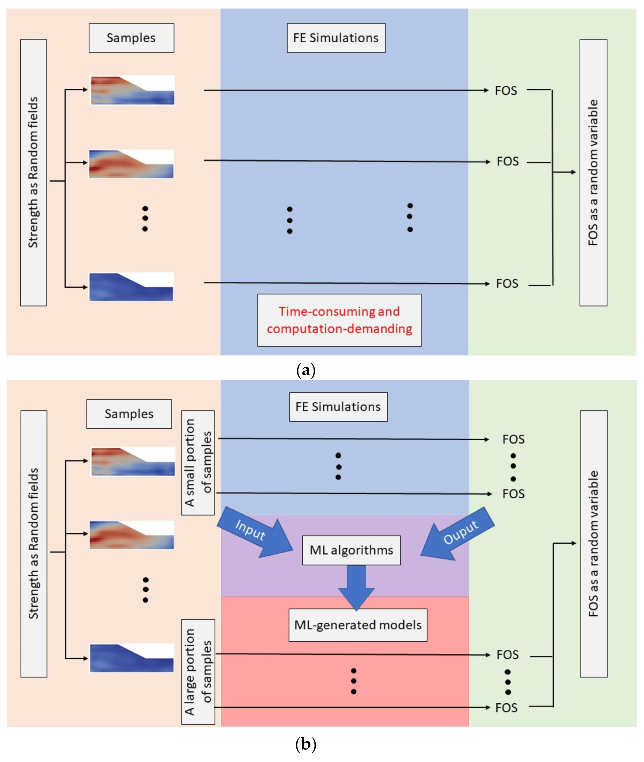
:1. Introduction
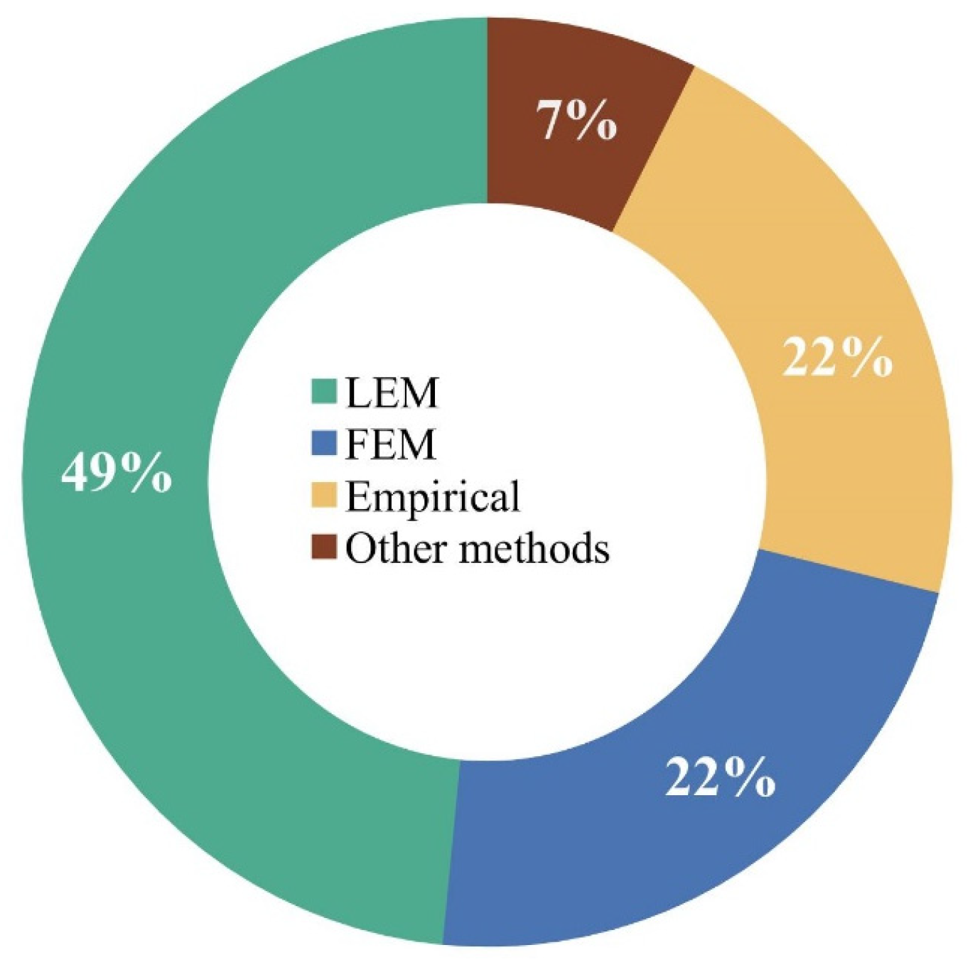
2. Brief Overview of Methods for Slope Stability Analysis
2.1. The Limit Equilibrium Method (LEM)
2.2. The Finite Element Method (FEM)
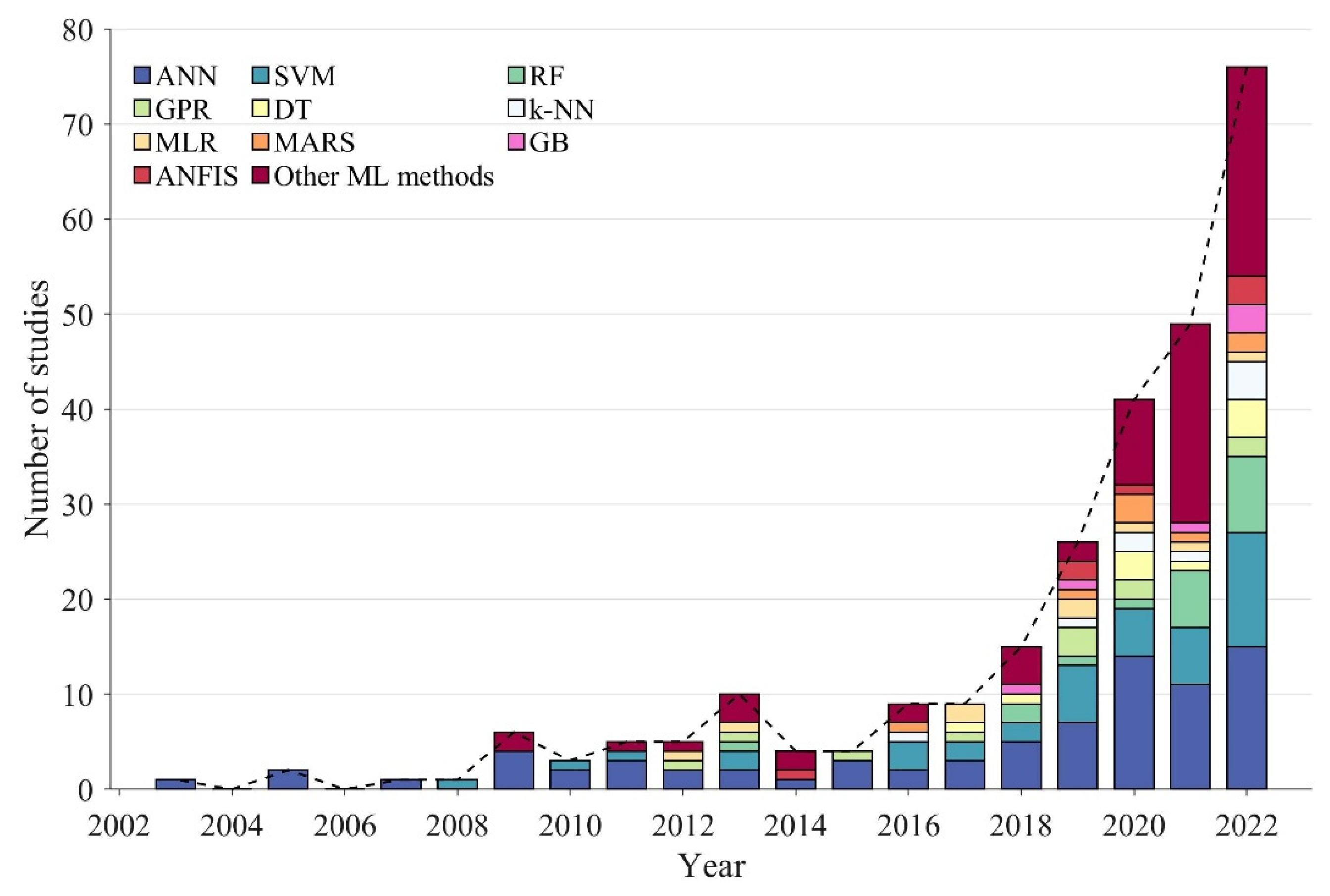
3. Brief Overview of Machine Learning (ML) Methods
3.1. Artificial Neural Networks (ANNs), Adaptive Neuro-Fuzzy Inference Systems (ANFISs), and Deep Neural Networks (DNNs)
- (1)
- The input data are transformed into fuzzy sets using membership functions.
- (2)
- The firing strength of each rule is generated from the input and rules.
- (3)
- Normalized firing strengths are calculated using weighted averaging.
- (4)
- Consequent parameters are adjusted to optimize the parameters and weights.
- (5)
- All incoming signals are summed up to obtain the overall output.
3.2. Support Vector Machine (SVM)
3.3. Gaussian Process Regression (GPR)
3.4. Decision Tree (DT), Random Forest (RF), and Gradient Boosting (GB)
3.5. K-Nearest Neighbor (k-NN)
3.6. Multilinear Regression (MLR) and Multivariate Adaptive Regression Splines (MARS)
- (1)
- Constant values (the intercept).
- (2)
- A hinge function:
- (3)
- A function of two or more hinge functions.
3.7. Some Other Machine Learning Methods
3.8. The Hyperparameter Optimization (HPO) Algorithm in Machine Learning
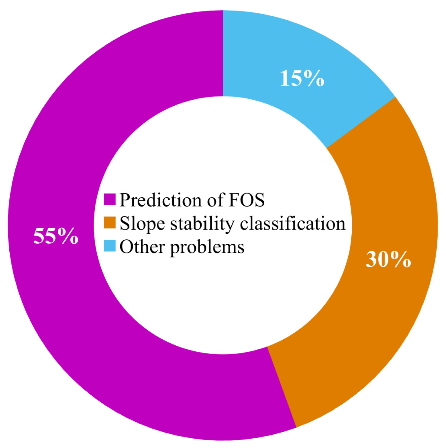
4. Application of ML Methods in Slope Stability
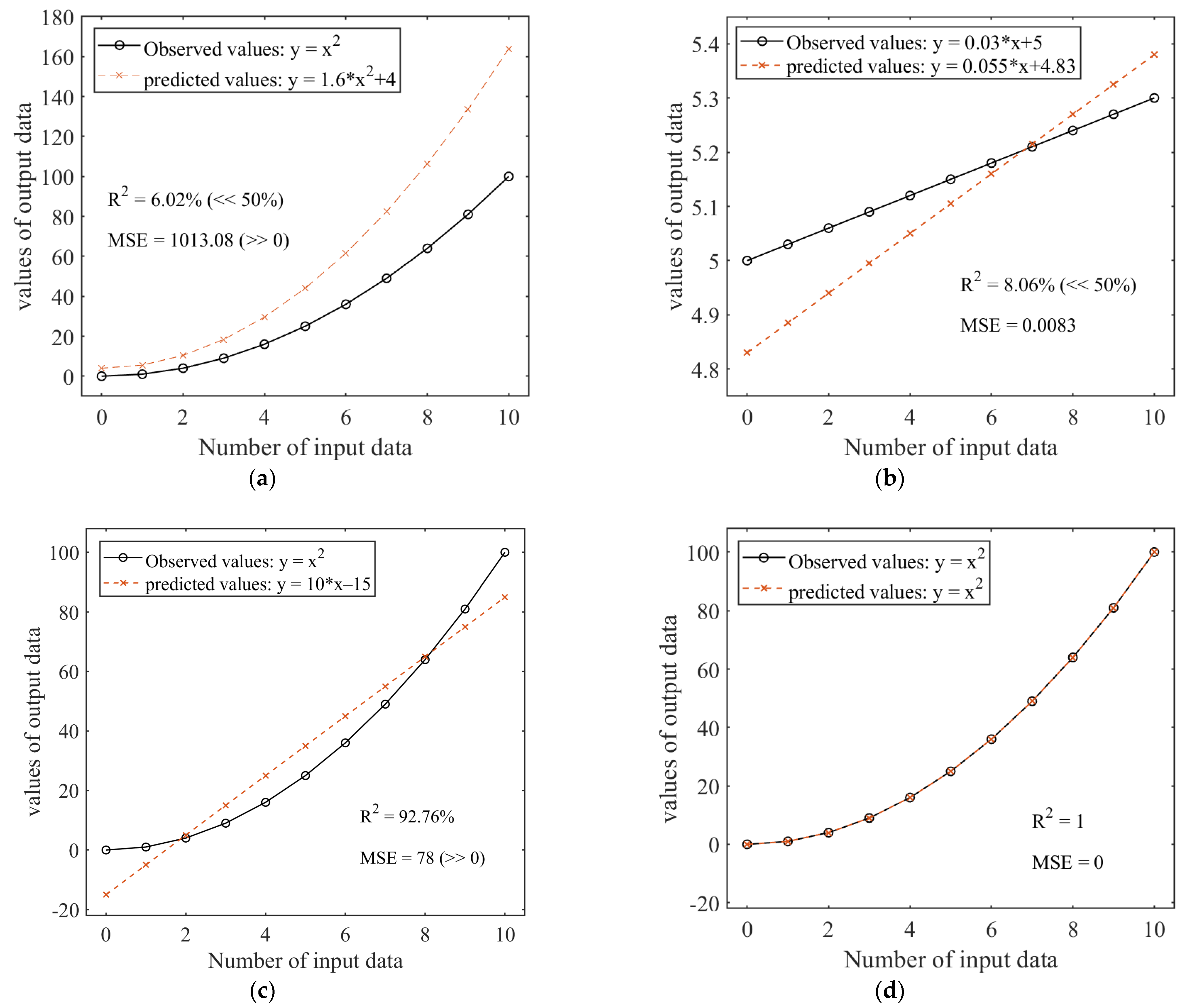
4.1. Performance Evaluation Metrics in Regression Problems Using Machine Learning
- (a)
- Low coefficient of determination and high error parameters. In this case, both the overall prediction and the individual predictions are unreliable, which may be due to outliers, such as wrong predictions of boundary values. In addition, non-linear relationships, heteroscedasticity, high noise, and overfitting/underfitting can also lead to this situation.
- (b)
- Low coefficient of determination and low error parameters. In this case, individual predictions are accurate, but the overall prediction is poor. One reason can be a low slope of the fitting function. Limited by the definition of R2, when the slope of the linear fitting function is low (the function value is close to the average value), even if the prediction accuracy is high, the calculation result of R2 tends to be 0. The model fails to account for the variability in these data. Similarly, non-linear relationships, heteroscedasticity, high noise, and overfitting/underfitting can also lead to this situation.
- (c)
- High coefficient of determination and high error parameters. In this case, the overall prediction is accurate, but the individual predictions are unreliable. This may be due to the use of a linear relationship to fit a non-linear function (incorrect fitting relationships). Uncertainty in the data, heteroscedasticity, outliers, and overfitting/underfitting can also lead to this situation. For example, if the data have large uncertainties, even if the model can explain some of the variance, the MSE may still be large due to the inherent uncertainty of the data.
- (d)
- High coefficient of determination and low error parameters. In this case, both the overall prediction and the individual predictions are good.

4.2. Failure Probability of Slopes
4.3. Prediction of the Factor of Safety
- (1)
- (2)
- Data collection and preprocessing: Random variables or random fields are mapped into numerical models, such as the LEM and FEM, and the associated FOS is calculated using the numerical models. All simulation results are required to be checked to ensure the correct FOS is obtained.
- (3)
- Model selection and training: One or more appropriate machine learning models are chosen based on the nature of the problem. A specific machine learning method is used to train and validate models with random variables or random fields as input and the FOS as output data. Trained models represent the nonlinear relationship between samples and the FOS. The conceptual function captured with machine learning is expressed as:
- (1)
- Model validation and tuning: The trained models are evaluated using either a validation or test dataset to assess their performance. Model parameters may be adjusted, or alternative models may be explored as necessary to attain the optimal model or a model that closely approaches optimality.
- (2)
- Model deployment: Based on the well-trained models, a large number of predicted FOS values can be quickly obtained, and the failure probability can be counted according to the predicted results.

| Reference | Method to Obtain FOS | ML Method | Input Variables | Dimension | Training Sample Size | Advantages | Limitations |
|---|---|---|---|---|---|---|---|
| Kang et al. (2016) [138] | LEM | ν-SVM | Case 1: , Case 2,3,4: | 2D | 20 | Good generalization capability; adaptable for high-dimensional problems | Single-prediction outputs |
| Ji et al. (2017) [139] | LEM | LS-SVM | , | 2D | 50–500 | Computationally efficient. good generalization capability; adaptable for high-dimensional problems | Single-prediction outputs |
| Mu’azu (2022) [61] | FEM | ANFIS, ANN | 2D | 504 | High accuracy; optimization methods for tuning hyperparameter | Time-consuming | |
| Ahangari Nanehkaran et al. (2022) [140] | LEM | ANN, DT, k-NN, RF, SVM | , , , , , , | 2D | 49 | Comparison of different machine-learning methods | Unable to determine generalization ability; requires large training sample size |
| Pandey et al. (2022) [105] | FDM | ANN, MLR | 2D | 148 | High accuracy | Unreliable samples are not excluded | |
| Hsiao et al. (2022) [65] | FEM | ANN, CNN | , , | 2D | Case1: 200 Case2: 400 | High accuracy; consideration of spatial variability; prediction of failure surface | Requires large training sample size |
| Jiang et al. (2022) [141] | LEM | GB | 2D | 37 | High accuracy; good generalization capability | Requires large memory; high sensitivity of hyperparameters | |
| Lin et al. (2021) [142] | LEM, empirical | ABR, Bagging, BR, ENR, ET, DT, k-NN, MLR, RF, SVM | , , , , , | 2D | 314 | Comparison of different machine-learning methods | Limited accuracy; no consideration of external or trigger factors |
| Falae et al. (2021) [106] | FEM | MARS | 2D | Section X-X′: 128, 256 Section Y-Y′: 512, 512 | Consideration of spatial variability | Requires known prior information; metric | |
| Cho (2009) [144] | FDM | ANN | , | 2D | Case1: 15–25 Case 2: 50–200 | High accuracy; parallel distributed processing; strong robustness | Requires a large number of initial parameters; consumes a lot of time during model training |
| Meng et al. (2021) [136] | FEM | ANN | 3D | Purely cohesive soil: 168 Cohesive-frictional soil:1254 | High accuracy; consideration of 3D geometries; consideration of concave slopes surface | Only valid for homogeneous dry slopes without pore pressure | |
| He et al. (2020) [31] | FEM | ANN, SVM | , , | 2D | 300 | High accuracy; consideration of spatial variability | Separate samples and training are required for each case |
| Ray et al. (2020) [145] | FEM, empirical | ANN | 2D | 320 | Consideration of weathering effects | Limited generalization capability; large number of input parameters | |
| Liu et al. (2019) [146] | LEM, FEM | MARS | , | 2D | Case1: 280 Case1: 210 | No need to deal with a large amount of data and high-dimension data | Unable to provide sequential prediction; single-prediction outputs |
| Wang et al. (2021) [67] | FEM | CNN | 2D | 5000 | Adaptable for high-dimensional problems; high performance in feature classification; efficiently handles large samples | Large number of samples required | |
| Suman et al. (2016) [143] | LEM | FN, MARS, MGGP | , , , , , | 2D | 75 | Prediction model equations are provided | No consideration of spatial variability |
4.4. Slope Stability Classification
5. Future Research Perspective
- (1)
- The spatial variation in shear strength parameters and hydraulic parameters is commonly considered in slope reliability and risk analysis. However, research on the hydro-mechanical coupling between these parameters is still limited. This means that the impact of rainfall or the groundwater table on slope stability is often not fully accounted for, as both hydraulic and shear strength parameters can have a significant influence.
- (2)
- Previous studies have mainly focused on simplified models, and there is a lack of realistic geotechnical engineering case applications. Moreover, most studies were limited to 2D slope simulations. Although 2D slope stability analysis has been extensively investigated, it neglects the effect of 3D spatial variation, which is a crucial factor in real-world applications. Despite being a technical challenge due to the larger computational efforts involved, several studies have demonstrated that 3D slope stability analysis results can significantly differ from those obtained using 2D models [136]. Therefore, future research should focus on analyzing existing 3D slope stability data using ML to provide more accurate and reliable results.
- (3)
- A site investigation often captures only one or two properties of material spatial variability, which can make it challenging to accurately estimate fluctuation scales and autocorrelations. The generation of random fields currently relies on selecting a theoretical autocorrelation function, which may not accurately represent the true fluctuation scale and autocorrelation in soil parameters. In the future, machine learning could potentially be utilized in field surveys to capture more realistic estimates of these parameters, leading to improved reliability in slope stability analysis.
- (4)
- Due to the ease of establishing and connecting databases, as well as the advances in monitoring technologies, it is anticipated that more comprehensive and detailed input data can be obtained for the slope stability classification problem, including environmental factors, meteorological information, and hydrogeological conditions. This will lead to more precise predictions of slope conditions.
6. Conclusions
Author Contributions
Funding
Data Availability Statement
Conflicts of Interest
Abbreviations
| ANFIS | adaptive neuro-fuzzy inference system | ANN | artificial neural network |
| BN | Bayesian network | CNN | convolutional neural network |
| DNN | deep neural network | DT | decision tree |
| FDM | finite difference method | FEM | finite element method |
| FOS | factor of safety | FN | functional network |
| GB | gradient boosting | GIM | gravity increasing method |
| GPR | Gaussian process regression | HPO | hyperparameter optimization |
| k-NN | k-nearest neighbor | LDC | linear discriminant classifier |
| LEM | limit equilibrium method | LS-SVM | least squares support vector machine |
| MAE | mean absolute error | MAPE | mean absolute percentage error |
| MARS | multivariate adaptive regression splines | MCS | Monte Carlo simulation |
| MDMSE | margin distance minimization selective ensemble | MGGP | multigene genetic programming |
| ML | machine learning | MLR | multilinear regression |
| MSE | mean squared error | probability density function | |
| QDC | quadratic discriminant classifier | coefficient of determination | |
| RF | random forest | RMSE | root mean square error |
| RSM | response surface method | SPCE | sparse polynomial chaos expansion |
| SPH | smoothed-particle hydrodynamics | SRM | strength reduction method |
| SVM | support vector machine | TLBO | teaching–learning-based optimization |
| ν-SVM | ν-support vector machine |
Notations
| Undrained shear strength | Pore pressure ratio | ||
| Slope angle | Poisson’s ratio | ||
| External force on the footing | Elastic modulus | ||
| Ratio of setback distance | Width ratio | ||
| Water content | Dimensionless group | ||
| Specific gravity | Young’s modulus of residual soil | ||
| Dry density | Cohesion of residual soil | ||
| Slope height | Friction of residual soil | ||
| Cohesion | Young’s modulus of rock mass | ||
| Friction angle | Cohesion of rock mass | ||
| Unit weight | Friction of rock mass | ||
| Rainfall intensity | Cohesion of joint interface | ||
| Rainfall duration | Friction of joint interface | ||
| Depth ratio | Front and back edge elevations | ||
| Inclination angle | Dip direction | ||
| Landslide volume | Categorical variables | ||
| Earthquake intensity | Ground water level |
References
- Meyerhof, G.G. Limit Analysis and Soil Plasticity, W.F. Chen (Ed.), Elsevier, Amsterdam (1975), p. 638 Dfl. 240.00. Eng. Geol. 1976, 10, 79. [Google Scholar] [CrossRef]
- Sloan, S.W. Lower Bound Limit Analysis Using Finite Elements and Linear Programming. Int. J. Numer. Anal. Methods Geomech. 1988, 12, 61–77. [Google Scholar] [CrossRef]
- Dawson, E.M.; Roth, W.H.; Drescher, A. Slope Stability Analysis by Strength Reduction. Géotechnique 1999, 49, 835–840. [Google Scholar] [CrossRef]
- Griffiths, D.V.; Lane, P.A. Slope Stability Analysis by Finite Elements. Géotechnique 1999, 49, 387–403. [Google Scholar] [CrossRef]
- Kaur, A.; Sharma, R.K. Slope Stability Analysis Techniques: A Review. Int. J. Eng. Appl. Sci. Technol. 2016, 1, 52–57. [Google Scholar]
- Pourkhosravani, A.; Kalantari, B. A Review of Current Methods for Slope Stability Evaluation. Electron. J. Geotech. Eng. 2011, 16, 1245–1254. [Google Scholar]
- Wallace, M.I.; Ng, K.C. Development and Application of Underground Space Use in Hong Kong. Tunn. Undergr. Space Technol. 2016, 55, 257–279. [Google Scholar] [CrossRef]
- Wei, X.; Zhang, L.; Yang, H.-Q.; Zhang, L.; Yao, Y.-P. Machine Learning for Pore-Water Pressure Time-Series Prediction: Application of Recurrent Neural Networks. Geosci. Front. 2021, 12, 453–467. [Google Scholar] [CrossRef]
- Zhang, J.; Tang, W.H.; Zhang, L.M. Efficient Probabilistic Back-Analysis of Slope Stability Model Parameters. J. Geotech. Geoenviron. Eng. 2010, 136, 99–109. [Google Scholar] [CrossRef]
- Zhang, W.; Li, H.; Han, L.; Chen, L.; Wang, L. Slope Stability Prediction Using Ensemble Learning Techniques: A Case Study in Yunyang County, Chongqing, China. J. Rock Mech. Geotech. Eng. 2022, 14, 1089–1099. [Google Scholar] [CrossRef]
- Wesley, L.D.; Leelaratnam, V. Shear Strength Parameters from Back-Analysis of Single Slips. Géotechnique 2001, 51, 373–374. [Google Scholar] [CrossRef]
- Tiwari, B.; Brandon, T.L.; Marui, H.; Tuladhar, G.R. Comparison of Residual Shear Strengths from Back Analysis and Ring Shear Tests on Undisturbed and Remolded Specimens. J. Geotech. Geoenviron. Eng. 2005, 131, 1071–1079. [Google Scholar] [CrossRef]
- Griffiths, D.V.; Fenton, G.A. Bearing Capacity of Spatially Random Soil: The Undrained Clay Prandtl Problem Revisited. Géotechnique 2001, 51, 351–359. [Google Scholar] [CrossRef]
- Sun, X.; Zeng, P.; Li, T.; Wang, S.; Jimenez, R.; Feng, X.; Xu, Q. From Probabilistic Back Analyses to Probabilistic Run-out Predictions of Landslides: A Case Study of Heifangtai Terrace, Gansu Province, China. Eng. Geol. 2021, 280, 105950. [Google Scholar] [CrossRef]
- He, X.; Wang, F.; Li, W.; Sheng, D. Deep Learning for Efficient Stochastic Analysis with Spatial Variability. Acta Geotech. 2022, 17, 1031–1051. [Google Scholar] [CrossRef]
- Ling, Q.; Zhang, Q.; Wei, Y.; Kong, L.; Zhu, L. Slope Reliability Evaluation Based on Multi-Objective Grey Wolf Optimization-Multi-Kernel-Based Extreme Learning Machine Agent Model. Bull. Eng. Geol. Environ. 2021, 80, 2011–2024. [Google Scholar] [CrossRef]
- Li, J.-Z.; Zhang, S.-H.; Liu, L.-L.; Huang, L.; Cheng, Y.-M.; Dias, D. Probabilistic Analysis of Pile-Reinforced Slopes in Spatially Variable Soils with Rotated Anisotropy. Comput. Geotech. 2022, 146, 104744. [Google Scholar] [CrossRef]
- Allaix, D.L.; Carbone, V.I. An Improvement of the Response Surface Method. Struct. Saf. 2011, 33, 165–172. [Google Scholar] [CrossRef]
- Wong, F.S. Slope Reliability and Response Surface Method. J. Geotech. Eng. 1985, 111, 32–53. [Google Scholar] [CrossRef]
- Kaymaz, I.; McMahon, C.A. A Response Surface Method Based on Weighted Regression for Structural Reliability Analysis. Probabilistic Eng. Mech. 2005, 20, 11–17. [Google Scholar] [CrossRef]
- Kim, S.-H.; Na, S.-W. Response Surface Method Using Vector Projected Sampling Points. Struct. Saf. 1997, 19, 3–19. [Google Scholar] [CrossRef]
- Desai, K.M.; Survase, S.A.; Saudagar, P.S.; Lele, S.S.; Singhal, R.S. Comparison of Artificial Neural Network (ANN) and Response Surface Methodology (RSM) in Fermentation Media Optimization: Case Study of Fermentative Production of Scleroglucan. Biochem. Eng. J. 2008, 41, 266–273. [Google Scholar] [CrossRef]
- Abbasi, B.; Mahlooji, H. Improving Response Surface Methodology by Using Artificial Neural Network and Simulated Annealing. Expert Syst. Appl. 2012, 39, 3461–3468. [Google Scholar] [CrossRef]
- Yang, H.-Q.; Zhang, L.; Pan, Q.; Phoon, K.-K.; Shen, Z. Bayesian Estimation of Spatially Varying Soil Parameters with Spatiotemporal Monitoring Data. Acta Geotech. 2021, 16, 263–278. [Google Scholar] [CrossRef]
- Liu, X.; Wang, Y.; Koo, R.C.H.; Kwan, J.S.H. Development of a Slope Digital Twin for Predicting Temporal Variation of Rainfall-Induced Slope Instability Using Past Slope Performance Records and Monitoring Data. Eng. Geol. 2022, 308, 106825. [Google Scholar] [CrossRef]
- Zeng, P.; Zhang, T.; Li, T.; Jimenez, R.; Zhang, J.; Sun, X. Binary Classification Method for Efficient and Accurate System Reliability Analyses of Layered Soil Slopes. Georisk Assess. Manag. Risk Eng. Syst. Geohazards 2022, 16, 435–451. [Google Scholar] [CrossRef]
- Hanandeh, S. Evaluation Circular Failure of Soil Slopes Using Classification and Predictive Gene Expression Programming Schemes. Front. Built Env. 2022, 8, 30. [Google Scholar] [CrossRef]
- Lin, Y.; Zhou, K.; Li, J. Prediction of Slope Stability Using Four Supervised Learning Methods. IEEE Access 2018, 6, 31169–31179. [Google Scholar] [CrossRef]
- Zhou, J.; Li, E.; Yang, S.; Wang, M.; Shi, X.; Yao, S.; Mitri, H.S. Slope Stability Prediction for Circular Mode Failure Using Gradient Boosting Machine Approach Based on an Updated Database of Case Histories. Saf. Sci. 2019, 118, 505–518. [Google Scholar] [CrossRef]
- Pham, K.; Kim, D.; Park, S.; Choi, H. Ensemble Learning-Based Classification Models for Slope Stability Analysis. Catena 2021, 196, 104886. [Google Scholar] [CrossRef]
- He, X.; Xu, H.; Sabetamal, H.; Sheng, D. Machine Learning Aided Stochastic Reliability Analysis of Spatially Variable Slopes. Comput. Geotech. 2020, 126, 103711. [Google Scholar] [CrossRef]
- Zhu, H.; Azarafza, M.; Akgün, H. Deep Learning-Based Key-Block Classification Framework for Discontinuous Rock Slopes. J. Rock Mech. Geotech. Eng. 2022, 14, 1131–1139. [Google Scholar] [CrossRef]
- Bello, O.; Holzmann, J.; Yaqoob, T.; Teodoriu, C. Application of Artificial Intelligence Methods in Drilling System Design and Operations: A Review of the State of the Art. J. Artif. Intell. Soft Comput. Res. 2015, 5, 121–139. [Google Scholar] [CrossRef]
- Nonoyama, H.; Moriguchi, S.; Sawada, K.; Yashima, A. Slope Stability Analysis Using Smoothed Particle Hydrodynamics (SPH) Method. Soils Found. 2015, 55, 458–470. [Google Scholar] [CrossRef]
- Bui, H.H.; Fukagawa, R.; Sako, K.; Wells, J.C. Slope Stability Analysis and Discontinuous Slope Failure Simulation by Elasto-Plastic Smoothed Particle Hydrodynamics (SPH). Géotechnique 2011, 61, 565–574. [Google Scholar] [CrossRef]
- He, X.; Liang, D.; Bolton, M.D. Run-out of Cut-Slope Landslides: Mesh-Free Simulations. Géotechnique 2018, 68, 50–63. [Google Scholar] [CrossRef]
- He, X.; Liang, D.; Wu, W.; Cai, G.; Zhao, C.; Wang, S. Study of the Interaction between Dry Granular Flows and Rigid Barriers with an SPH Model. Int. J. Numer. Anal. Methods Geomech. 2018, 42, 1217–1234. [Google Scholar] [CrossRef]
- Fredlund, D.G. Analytical Methods for Slope Stability Analysis. In Proceedings of the 4th International Symposium on Landslides, Toronto, ON, Canada, 16–21 September 1984; Volume 250. [Google Scholar]
- Bishop, A.W. The Use of the Slip Circle in the Stability Analysis of Slopes. Géotechnique 1955, 5, 7–17. [Google Scholar] [CrossRef]
- Kalatehjari, R.; Ali, N. A Review of Three-Dimensional Slope Stability Analyses Based on Limit Equilibrium Method. Electron. J. Geotech. Eng. 2013, 18, 119–134. [Google Scholar]
- Abramson, L.W.; Lee, T.S.; Sharma, S.; Boyce, G.M. Slope Stability and Stabilization Methods; John Wiley & Sons: Hoboken, NJ, USA, 2001; ISBN 0471384933. [Google Scholar]
- Zhu, D.Y.; Lee, C.F.; Jiang, H.D.; Lee, C.F.; Iang, H.D.J. Generalised Framework of Limit Equilibrium Methods for Slope Stability Analysis. Géotechnique 2003, 53, 377–395. [Google Scholar] [CrossRef]
- Zienkiewicz, O.C.; Taylor, R.L.; Zhu, J.Z. The Finite Element Method: Its Basis and Fundamentals; Elsevier: Amsterdam, The Netherlands, 2005; ISBN 008047277X. [Google Scholar]
- Belytschko, T.; Liu, W.K.; Moran, B.; Elkhodary, K. Nonlinear Finite Elements for Continua and Structures; John wiley & Sons: Hoboken, NJ, USA, 2014; ISBN 1118632702. [Google Scholar]
- Bathe, K.-J. Finite Element Procedures; Klaus-Jurgen Bathe: Cambridge, MA, USA, 2006; ISBN 097900490X. [Google Scholar]
- Matsui, T.; San, K.-C. Finite Element Slope Stability Analysis by Shear Strength Reduction Technique. Soils Found. 1992, 32, 59–70. [Google Scholar] [CrossRef]
- Cheng, Y.M.; Lansivaara, T.; Wei, W.B. Two-Dimensional Slope Stability Analysis by Limit Equilibrium and Strength Reduction Methods. Comput. Geotech. 2007, 34, 137–150. [Google Scholar] [CrossRef]
- Sternik, K. Comparison of Slope Stability Predictions by Gravity Increase and Shear Strength Reduction Methods. Czas. Tech. Sr. 2013, 110, 121–130. [Google Scholar]
- Baghbani, A.; Choudhury, T.; Costa, S.; Reiner, J. Application of Artificial Intelligence in Geotechnical Engineering: A State-of-the-Art Review. Earth Sci. Rev. 2022, 228, 103991. [Google Scholar] [CrossRef]
- Zhang, H.; Nguyen, H.; Bui, X.-N.; Pradhan, B.; Asteris, P.G.; Costache, R.; Aryal, J. A Generalized Artificial Intelligence Model for Estimating the Friction Angle of Clays in Evaluating Slope Stability Using a Deep Neural Network and Harris Hawks Optimization Algorithm. Eng. Comput. 2021, 38, 3901–3914. [Google Scholar] [CrossRef]
- Wang, H.; Moayedi, H.; Kok Foong, L. Genetic Algorithm Hybridized with Multilayer Perceptron to Have an Economical Slope Stability Design. Eng. Comput. 2021, 37, 3067–3078. [Google Scholar] [CrossRef]
- Yuan, C.; Moayedi, H. Evaluation and Comparison of the Advanced Metaheuristic and Conventional Machine Learning Methods for the Prediction of Landslide Occurrence. Eng. Comput. 2020, 36, 1801–1811. [Google Scholar] [CrossRef]
- Liu, Z.; Shao, J.; Xu, W.; Chen, H.; Zhang, Y. An Extreme Learning Machine Approach for Slope Stability Evaluation and Prediction. Nat. Hazards 2014, 73, 787–804. [Google Scholar] [CrossRef]
- Kang, F.; Li, J.-S.; Wang, Y.; Li, J. Extreme Learning Machine-Based Surrogate Model for Analyzing System Reliability of Soil Slopes. Eur. J. Environ. Civ. Eng. 2017, 21, 1341–1362. [Google Scholar] [CrossRef]
- Hornik, K.; Stinchcombe, M.; White, H. Multilayer Feedforward Networks Are Universal Approximators. Neural Netw. 1989, 2, 359–366. [Google Scholar] [CrossRef]
- Palmer, A.; Montano, J.J.; Sesé, A. Designing an Artificial Neural Network for Forecasting Tourism Time Series. Tour. Manag. 2006, 27, 781–790. [Google Scholar] [CrossRef]
- Ghiassi, M.; Saidane, H.; Zimbra, D.K. A Dynamic Artificial Neural Network Model for Forecasting Time Series Events. Int. J. Forecast. 2005, 21, 341–362. [Google Scholar] [CrossRef]
- Billsus, D.; Pazzani, M.J. Learning Collaborative Information Filters. In Proceedings of the Fifteenth International Conference on Machine Learning, Madison, WI, USA, 24–27 July 1998; Volume 98, pp. 46–54. [Google Scholar]
- Jang, J.-S. ANFIS: Adaptive-Network-Based Fuzzy Inference System. IEEE Trans. Syst. Man Cybern. 1993, 23, 665–685. [Google Scholar] [CrossRef]
- Jang, J.-S.R. Fuzzy Modeling Using Generalized Neural Networks and Kalman Filter Algorithm. In Proceedings of the AAAI, Anaheim, CA, USA, 14–19 July 1991; Volume 91, pp. 762–767. [Google Scholar]
- Mu’azu, M.A. Enhancing Slope Stability Prediction Using Fuzzy and Neural Frameworks Optimized by Metaheuristic Science. Math. Geosci. 2022, 55, 263–285. [Google Scholar] [CrossRef]
- Al-Mahasneh, M.; Aljarrah, M.; Rababah, T.; Alu’datt, M. Application of Hybrid Neural Fuzzy System (ANFIS) in Food Processing and Technology. Food Eng. Rev. 2016, 8, 351–366. [Google Scholar] [CrossRef]
- Szegedy, C.; Liu, W.; Jia, Y.; Sermanet, P.; Reed, S.; Anguelov, D.; Erhan, D.; Vanhoucke, V.; Rabinovich, A. Going Deeper with Convolutions. In Proceedings of the IEEE Conference on Computer Vision and Pattern Recognition, Boston, MA, USA, 7–12 June 2015; pp. 1–9. [Google Scholar]
- He, X.; Xu, H.; Sheng, D. Ready-to-Use Deep-Learning Surrogate Models for Problems with Spatially Variable Inputs and Outputs. Acta Geotech. 2022, 18, 1681–1698. [Google Scholar] [CrossRef]
- Hsiao, C.-H.; Chen, A.Y.; Ge, L.; Yeh, F.-H. Performance of Artificial Neural Network and Convolutional Neural Network on Slope Failure Prediction Using Data from the Random Finite Element Method. Acta Geotech. 2022, 17, 5801–5811. [Google Scholar] [CrossRef]
- Xu, H.; He, X.; Pradhan, B.; Sheng, D. A Pre-Trained Deep-Learning Surrogate Model for Slope Stability Analysis with Spatial Variability. Soils Found. 2023, 63, 101321. [Google Scholar] [CrossRef]
- Wang, Z.-Z.; Goh, S.H. Novel Approach to Efficient Slope Reliability Analysis in Spatially Variable Soils. Eng. Geol. 2021, 281, 105989. [Google Scholar] [CrossRef]
- Mikolov, T.; Karafiát, M.; Burget, L.; Cernocký, J.; Khudanpur, S. Recurrent Neural Network Based Language Model. In Proceedings of the Interspeech, Makuhari, Japan, 26–30 September 2010; Volume 2, pp. 1045–1048. [Google Scholar]
- Graves, A.; Mohamed, A.; Hinton, G. Speech Recognition with Deep Recurrent Neural Networks. In Proceedings of the 2013 IEEE International Conference on Acoustics, Speech and Signal Processing, Vancouver, BC, Canada, 26–31 May 2013; IEEE: New York, NY, USA, 2013; pp. 6645–6649. [Google Scholar]
- Brown, T.; Mann, B.; Ryder, N.; Subbiah, M.; Kaplan, J.D.; Dhariwal, P.; Neelakantan, A.; Shyam, P.; Sastry, G.; Askell, A. Language Models Are Few-Shot Learners. Adv. Neural Inf. Process. Syst. 2020, 33, 1877–1901. [Google Scholar]
- Boser, B.E.; Guyon, I.M.; Vapnik, V.N. A Training Algorithm for Optimal Margin Classifiers. In Proceedings of the Fifth Annual Workshop on Computational Learning Theory, Pittsburgh, PA, USA, 27–29 July 1992; pp. 144–152. [Google Scholar]
- Sun, A.; Lim, E.-P.; Ng, W.-K. Web Classification Using Support Vector Machine. In Proceedings of the 4th International Workshop on Web Information and Data Management, McLean, VA, USA, 8 November 2002; pp. 96–99. [Google Scholar]
- Byvatov, E.; Schneider, G. Support Vector Machine Applications in Bioinformatics. Appl. Bioinform. 2003, 2, 67–77. [Google Scholar]
- Venkatesan, C.; Karthigaikumar, P.; Paul, A.; Satheeskumaran, S.; Kumar, R. ECG Signal Preprocessing and SVM Classifier-Based Abnormality Detection in Remote Healthcare Applications. IEEE Access 2018, 6, 9767–9773. [Google Scholar] [CrossRef]
- Mahmoodzadeh, A.; Mohammadi, M.; Ibrahim, H.H.; Rashid, T.A.; Aldalwie, A.H.M.; Ali, H.F.H.; Daraei, A. Tunnel Geomechanical Parameters Prediction Using Gaussian Process Regression. Mach. Learn. Appl. 2021, 3, 100020. [Google Scholar] [CrossRef]
- Zhu, B.; Hiraishi, T.; Pei, H.; Yang, Q. Efficient Reliability Analysis of Slopes Integrating the Random Field Method and a Gaussian Process Regression-based Surrogate Model. Int. J. Numer. Anal. Methods Geomech. 2021, 45, 478–501. [Google Scholar] [CrossRef]
- Kang, F.; Han, S.; Salgado, R.; Li, J. System Probabilistic Stability Analysis of Soil Slopes Using Gaussian Process Regression with Latin Hypercube Sampling. Comput. Geotech. 2015, 63, 13–25. [Google Scholar] [CrossRef]
- Wang, C.; Wu, X.; Kozlowski, T. Gaussian Process–Based Inverse Uncertainty Quantification for Trace Physical Model Parameters Using Steady-State Psbt Benchmark. Nucl. Sci. Eng. 2019, 193, 100–114. [Google Scholar] [CrossRef]
- Kang, F.; Xu, B.; Li, J.; Zhao, S. Slope Stability Evaluation Using Gaussian Processes with Various Covariance Functions. Appl. Soft Comput. 2017, 60, 387–396. [Google Scholar] [CrossRef]
- Snoek, J.; Larochelle, H.; Adams, R.P. Practical Bayesian Optimization of Machine Learning Algorithms. Adv. Neural Inf. Process. Syst. 2012, 25, 2951–2959. [Google Scholar]
- Frazier, P.I. A Tutorial on Bayesian Optimization. arXiv 2018, arXiv:1807.02811. [Google Scholar]
- Kardani, N.; Zhou, A.; Nazem, M.; Shen, S.-L. Improved Prediction of Slope Stability Using a Hybrid Stacking Ensemble Method Based on Finite Element Analysis and Field Data. J. Rock Mech. Geotech. Eng. 2021, 13, 188–201. [Google Scholar] [CrossRef]
- Pekel, E. Estimation of Soil Moisture Using Decision Tree Regression. Theor. Appl. Clim. 2020, 139, 1111–1119. [Google Scholar] [CrossRef]
- Gareth, J.; Daniela, W.; Trevor, H.; Robert, T. An Introduction to Statistical Learning: With Applications in R; Spinger: Berlin/Heidelberg, Germany, 2013. [Google Scholar]
- Ben-Gal, I.; Dana, A.; Shkolnik, N.; Singer, G. Efficient Construction of Decision Trees by the Dual Information Distance Method. Qual. Technol. Quant. Manag. 2014, 11, 133–147. [Google Scholar] [CrossRef]
- Breiman, L. Random Forests. Mach. Learn. 2001, 45, 5–32. [Google Scholar] [CrossRef]
- Nath, S.K.; Sengupta, A.; Srivastava, A. Remote Sensing GIS-Based Landslide Susceptibility & Risk Modeling in Darjeeling–Sikkim Himalaya Together with FEM-Based Slope Stability Analysis of the Terrain. Nat. Hazards 2021, 108, 3271–3304. [Google Scholar]
- Ziegler, A.; König, I.R. Mining Data with Random Forests: Current Options for Real-world Applications. Wiley Interdiscip. Rev. Data Min. Knowl. Discov. 2014, 4, 55–63. [Google Scholar] [CrossRef]
- Shah, A.D.; Bartlett, J.W.; Carpenter, J.; Nicholas, O.; Hemingway, H. Comparison of Random Forest and Parametric Imputation Models for Imputing Missing Data Using MICE: A CALIBER Study. Am. J. Epidemiol. 2014, 179, 764–774. [Google Scholar] [CrossRef]
- Mendez, G.; Lohr, S. Estimating Residual Variance in Random Forest Regression. Comput. Stat. Data Anal. 2011, 55, 2937–2950. [Google Scholar] [CrossRef]
- Piryonesi, S.M.; El-Diraby, T.E. Data Analytics in Asset Management: Cost-Effective Prediction of the Pavement Condition Index. J. Infrastruct. Syst. 2020, 26, 04019036. [Google Scholar] [CrossRef]
- Hastie, T.; Tibshirani, R.; Friedman, J.; Hastie, T.; Tibshirani, R.; Friedman, J. Boosting and Additive Trees. Elem. Stat. Learn. Data Min. Inference Predict. 2009, 103, 337–387. [Google Scholar]
- Karir, D.; Ray, A.; Bharati, A.K.; Chaturvedi, U.; Rai, R.; Khandelwal, M. Stability Prediction of a Natural and Man-Made Slope Using Various Machine Learning Algorithms. Transp. Geotech. 2022, 34, 100745. [Google Scholar] [CrossRef]
- Madeh Piryonesi, S.; El-Diraby, T.E. Using Machine Learning to Examine Impact of Type of Performance Indicator on Flexible Pavement Deterioration Modeling. J. Infrastruct. Syst. 2021, 27, 04021005. [Google Scholar] [CrossRef]
- Soni, J.; Ansari, U.; Sharma, D.; Soni, S. Predictive Data Mining for Medical Diagnosis: An Overview of Heart Disease Prediction. Int. J. Comput. Appl. 2011, 17, 43–48. [Google Scholar] [CrossRef]
- Brown, I.; Mues, C. An Experimental Comparison of Classification Algorithms for Imbalanced Credit Scoring Data Sets. Expert Syst. Appl. 2012, 39, 3446–3453. [Google Scholar] [CrossRef]
- Peterson, L.E. K-Nearest Neighbor. Scholarpedia 2009, 4, 1883. [Google Scholar] [CrossRef]
- Mahmoodzadeh, A.; Mohammadi, M.; Farid Hama Ali, H.; Hashim Ibrahim, H.; Nariman Abdulhamid, S.; Nejati, H.R. Prediction of Safety Factors for Slope Stability: Comparison of Machine Learning Techniques. Nat. Hazards 2022, 111, 1771–1799. [Google Scholar] [CrossRef]
- Bhatia, N. Survey of Nearest Neighbor Techniques. arXiv 2010, arXiv:1007.0085. [Google Scholar]
- Zhang, H.; Berg, A.C.; Maire, M.; Malik, J. SVM-KNN: Discriminative Nearest Neighbor Classification for Visual Category Recognition. In Proceedings of the 2006 IEEE Computer Society Conference on Computer Vision and Pattern Recognition (CVPR’06), New York, NY, USA, 17–22 June 2006; IEEE: New York, NY, USA, 2006; Volume 2, pp. 2126–2136. [Google Scholar]
- Homaeinezhad, M.R.; Atyabi, S.A.; Tavakkoli, E.; Toosi, H.N.; Ghaffari, A.; Ebrahimpour, R. ECG Arrhythmia Recognition via a Neuro-SVM–KNN Hybrid Classifier with Virtual QRS Image-Based Geometrical Features. Expert Syst. Appl. 2012, 39, 2047–2058. [Google Scholar] [CrossRef]
- Trstenjak, B.; Mikac, S.; Donko, D. KNN with TF-IDF Based Framework for Text Categorization. Procedia Eng. 2014, 69, 1356–1364. [Google Scholar] [CrossRef]
- Tan, S. An Effective Refinement Strategy for KNN Text Classifier. Expert Syst. Appl. 2006, 30, 290–298. [Google Scholar] [CrossRef]
- Adeniyi, D.A.; Wei, Z.; Yongquan, Y. Automated Web Usage Data Mining and Recommendation System Using K-Nearest Neighbor (KNN) Classification Method. Appl. Comput. Inform. 2016, 12, 90–108. [Google Scholar] [CrossRef]
- Pandey, V.H.R.; Kainthola, A.; Sharma, V.; Srivastav, A.; Jayal, T.; Singh, T.N. Deep Learning Models for Large-Scale Slope Instability Examination in Western Uttarakhand, India. Environ. Earth Sci. 2022, 81, 487. [Google Scholar] [CrossRef]
- Falae, P.O.; Agarwal, E.; Pain, A.; Dash, R.K.; Kanungo, D.P. A Data Driven Efficient Framework for the Probabilistic Slope Stability Analysis of Pakhi Landslide, Garhwal Himalaya. J. Earth Syst. Sci. 2021, 130, 167. [Google Scholar] [CrossRef]
- Zhang, W.; Goh, A.T.C. Multivariate Adaptive Regression Splines and Neural Network Models for Prediction of Pile Drivability. Geosci. Front. 2016, 7, 45–52. [Google Scholar] [CrossRef]
- Friedman, J.H.; Roosen, C.B. An Introduction to Multivariate Adaptive Regression Splines. Stat. Methods Med. Res. 1995, 4, 197–217. [Google Scholar] [CrossRef] [PubMed]
- Lee, T.-S.; Chiu, C.-C.; Chou, Y.-C.; Lu, C.-J. Mining the Customer Credit Using Classification and Regression Tree and Multivariate Adaptive Regression Splines. Comput. Stat. Data Anal. 2006, 50, 1113–1130. [Google Scholar] [CrossRef]
- Lee, T.-S.; Chen, I.-F. A Two-Stage Hybrid Credit Scoring Model Using Artificial Neural Networks and Multivariate Adaptive Regression Splines. Expert Syst. Appl. 2005, 28, 743–752. [Google Scholar] [CrossRef]
- Leathwick, J.R.; Elith, J.; Hastie, T. Comparative Performance of Generalized Additive Models and Multivariate Adaptive Regression Splines for Statistical Modelling of Species Distributions. Ecol. Model. 2006, 199, 188–196. [Google Scholar] [CrossRef]
- Lewis, P.A.W.; Stevens, J.G. Nonlinear Modeling of Time Series Using Multivariate Adaptive Regression Splines (MARS). J. Am. Stat. Assoc. 1991, 86, 864–877. [Google Scholar] [CrossRef]
- Yang, H.-Q.; Yan, Y.; Wei, X.; Shen, Z.; Chen, X. Probabilistic Analysis of Highly Nonlinear Models by Adaptive Sparse Polynomial Chaos: Transient Infiltration in Unsaturated Soil. Int. J. Comput. Methods 2023, 20, 2350006. [Google Scholar] [CrossRef]
- Guo, X.; Dias, D.; Carvajal, C.; Peyras, L.; Breul, P. Reliability Analysis of Embankment Dam Sliding Stability Using the Sparse Polynomial Chaos Expansion. Eng. Struct. 2018, 174, 295–307. [Google Scholar] [CrossRef]
- Blatman, G.; Sudret, B. An Adaptive Algorithm to Build up Sparse Polynomial Chaos Expansions for Stochastic Finite Element Analysis. Probabilistic Eng. Mech. 2010, 25, 183–197. [Google Scholar] [CrossRef]
- Wang, J.; Gu, X.; Huang, T. Using Bayesian Networks in Analyzing Powerful Earthquake Disaster Chains. Nat. Hazards 2013, 68, 509–527. [Google Scholar] [CrossRef]
- Jensen, F.V.; Nielsen, T.D. Bayesian Networks and Decision Graphs; Springer: Berlin/Heidelberg, Germany, 2007; Volume 2. [Google Scholar]
- Kuhn, M.; Johnson, K. Applied Predictive Modeling; Springer: Berlin/Heidelberg, Germany, 2013; Volume 26. [Google Scholar]
- Montgomery, D.C. Design and Analysis of Experiments; John wiley & Sons: Hoboken, NJ, USA, 2017; ISBN 1119113474. [Google Scholar]
- Bergstra, J.; Bengio, Y. Random Search for Hyper-Parameter Optimization. J. Mach. Learn. Res. 2012, 13, 281–305. [Google Scholar]
- Xu, H.; He, X.; Sheng, D. Rainfall-Induced Landslides from Initialization to Post-Failure Flows: Stochastic Analysis with Machine Learning. Mathematics 2022, 10, 4426. [Google Scholar] [CrossRef]
- Phoon, K.-K.; Cao, Z.-J.; Ji, J.; Leung, Y.F.; Najjar, S.; Shuku, T.; Tang, C.; Yin, Z.-Y.; Ikumasa, Y.; Ching, J. Geotechnical Uncertainty, Modeling, and Decision Making. Soils Found. 2022, 62, 101189. [Google Scholar]
- Griffiths, D.V.; Huang, J.; Fenton, G.A. Influence of Spatial Variability on Slope Reliability Using 2-D Random Fields. J. Geotech. Geoenviron. Eng. 2009, 135, 1367–1378. [Google Scholar] [CrossRef]
- Li, D.-Q.; Jiang, S.-H.; Cao, Z.-J.; Zhou, W.; Zhou, C.-B.; Zhang, L.-M. A Multiple Response-Surface Method for Slope Reliability Analysis Considering Spatial Variability of Soil Properties. Eng. Geol. 2015, 187, 60–72. [Google Scholar] [CrossRef]
- Tan, X.; Shen, M.; Hou, X.; Li, D.; Hu, N. Response Surface Method of Reliability Analysis and Its Application in Slope Stability Analysis. Geotech. Geol. Eng. 2013, 31, 1011–1025. [Google Scholar] [CrossRef]
- Jiang, S.-H.; Huang, J.-S. Efficient Slope Reliability Analysis at Low-Probability Levels in Spatially Variable Soils. Comput. Geotech. 2016, 75, 18–27. [Google Scholar] [CrossRef]
- Li, D.-Q.; Zheng, D.; Cao, Z.-J.; Tang, X.-S.; Phoon, K.-K. Response Surface Methods for Slope Reliability Analysis: Review and Comparison. Eng. Geol. 2016, 203, 3–14. [Google Scholar] [CrossRef]
- Pontius, R.G.; Thontteh, O.; Chen, H. Components of Information for Multiple Resolution Comparison between Maps That Share a Real Variable. Environ. Ecol. Stat. 2008, 15, 111–142. [Google Scholar] [CrossRef]
- Shan, F.; He, X.; Xu, H.; Armaghani, D.J.; Sheng, D. Applications of Machine Learning in Mechanised Tunnel Construction: A Systematic Review. Eng 2023, 4, 1516–1535. [Google Scholar] [CrossRef]
- Frangopol, D.M. Probability Concepts in Engineering: Emphasis on Applications to Civil and Environmental Engineering; Wiley: Hoboken, NJ, USA, 2008. [Google Scholar]
- Jiang, S.-H.; Huang, J.; Griffiths, D.V.; Deng, Z.-P. Advances in Reliability and Risk Analyses of Slopes in Spatially Variable Soils: A State-of-the-Art Review. Comput. Geotech. 2022, 141, 104498. [Google Scholar]
- Fenton, G.A.; Griffiths, D.V. Risk Assessment in Geotechnical Engineering; John Wiley & Sons: New York, NY, USA, 2008; Volume 461. [Google Scholar]
- Zhang, J.; Ellingwood, B. Orthogonal Series Expansions of Random Fields in Reliability Analysis. J. Eng. Mech. 1994, 120, 2660–2677. [Google Scholar] [CrossRef]
- Betz, W.; Papaioannou, I.; Straub, D. Numerical Methods for the Discretization of Random Fields by Means of the Karhunen–Loève Expansion. Comput. Methods Appl. Mech. Eng. 2014, 271, 109–129. [Google Scholar] [CrossRef]
- Zhang, J.; Huang, H.W.; Phoon, K.K. Application of the Kriging-Based Response Surface Method to the System Reliability of Soil Slopes. J. Geotech. Geoenviron. Eng. 2013, 139, 651–655. [Google Scholar] [CrossRef]
- Meng, J.; Mattsson, H.; Laue, J. Three-dimensional Slope Stability Predictions Using Artificial Neural Networks. Int. J. Numer. Anal. Methods Geomech. 2021, 45, 1988–2000. [Google Scholar] [CrossRef]
- Song, L.; Yu, X.; Xu, B.; Pang, R.; Zhang, Z. 3D Slope Reliability Analysis Based on the Intelligent Response Surface Methodology. Bull. Eng. Geol. Environ. 2021, 80, 735–749. [Google Scholar] [CrossRef]
- Kang, F.; Xu, Q.; Li, J. Slope Reliability Analysis Using Surrogate Models via New Support Vector Machines with Swarm Intelligence. Appl. Math. Model. 2016, 40, 6105–6120. [Google Scholar] [CrossRef]
- Ji, J.; Zhang, C.; Gui, Y.; Lü, Q.; Kodikara, J. New Observations on the Application of LS-SVM in Slope System Reliability Analysis. J. Comput. Civ. Eng. 2017, 31, 06016002. [Google Scholar] [CrossRef]
- Ahangari Nanehkaran, Y.; Pusatli, T.; Chengyong, J.; Chen, J.; Cemiloglu, A.; Azarafza, M.; Derakhshani, R. Application of Machine Learning Techniques for the Estimation of the Safety Factor in Slope Stability Analysis. Water 2022, 14, 3743. [Google Scholar] [CrossRef]
- Jiang, S.; Li, J.; Zhang, S.; Gu, Q.; Lu, C.; Liu, H. Landslide Risk Prediction by Using GBRT Algorithm: Application of Artificial Intelligence in Disaster Prevention of Energy Mining. Process Saf. Environ. Prot. 2022, 166, 384–392. [Google Scholar] [CrossRef]
- Lin, S.; Zheng, H.; Han, C.; Han, B.; Li, W. Evaluation and Prediction of Slope Stability Using Machine Learning Approaches. Front. Struct. Civ. Eng. 2021, 15, 821–833. [Google Scholar] [CrossRef]
- Suman, S.; Khan, S.Z.; Das, S.K.; Chand, S.K. Slope Stability Analysis Using Artificial Intelligence Techniques. Nat. Hazards 2016, 84, 727–748. [Google Scholar] [CrossRef]
- Cho, S.E. Probabilistic Stability Analyses of Slopes Using the ANN-Based Response Surface. Comput. Geotech. 2009, 36, 787–797. [Google Scholar] [CrossRef]
- Ray, A.; Kumar, V.; Kumar, A.; Rai, R.; Khandelwal, M.; Singh, T.N. Stability Prediction of Himalayan Residual Soil Slope Using Artificial Neural Network. Nat. Hazards 2020, 103, 3523–3540. [Google Scholar] [CrossRef]
- Liu, L.; Zhang, S.; Cheng, Y.-M.; Liang, L. Advanced Reliability Analysis of Slopes in Spatially Variable Soils Using Multivariate Adaptive Regression Splines. Geosci. Front. 2019, 10, 671–682. [Google Scholar] [CrossRef]
- He, L.; Coggan, J.; Francioni, M.; Eyre, M. Maximizing Impacts of Remote Sensing Surveys in Slope Stability—A Novel Method to Incorporate Discontinuities into Machine Learning Landslide Prediction. ISPRS Int. J. Geoinf. 2021, 10, 232. [Google Scholar] [CrossRef]
- Zhang, H.; Wu, S.; Zhang, X.; Han, L.; Zhang, Z. Slope Stability Prediction Method Based on the Margin Distance Minimization Selective Ensemble. Catena 2022, 212, 106055. [Google Scholar] [CrossRef]
- Lin, S.; Zheng, H.; Han, B.; Li, Y.; Han, C.; Li, W. Comparative Performance of Eight Ensemble Learning Approaches for the Development of Models of Slope Stability Prediction. Acta Geotech. 2022, 17, 1477–1502. [Google Scholar] [CrossRef]
- Azmoon, B.; Biniyaz, A.; Liu, Z.; Sun, Y. Image-Data-Driven Slope Stability Analysis for Preventing Landslides Using Deep Learning. IEEE Access 2021, 9, 150623–150636. [Google Scholar] [CrossRef]
- Yuan, C.; Moayedi, H. The Performance of Six Neural-Evolutionary Classification Techniques Combined with Multi-Layer Perception in Two-Layered Cohesive Slope Stability Analysis and Failure Recognition. Eng. Comput. 2020, 36, 1705–1714. [Google Scholar] [CrossRef]
- Huang, S.; Huang, M.; Lyu, Y. An Improved KNN-Based Slope Stability Prediction Model. Adv. Civ. Eng. 2020, 2020, 8894109. [Google Scholar] [CrossRef]
- Ospina-Dávila, Y.M.; Orozco-Alzate, M. Parsimonious Design of Pattern Recognition Systems for Slope Stability Analysis. Earth Sci. Inform. 2020, 13, 523–536. [Google Scholar] [CrossRef]


| Reference | Method Classification | ML Method | Input Variables | Training Sample Size | Advantages | Limitations |
|---|---|---|---|---|---|---|
| Zhang et al. (2022) [10] | Empirical method | RF, XGboost, SVM, LR | 628 | High accuracy; good generalization capability | Requires large memory; large number of samples required | |
| Zhu et al. (2022) [32] | Empirical method | ANN, BNB, CNN, DT, GNB, RF, SVM | High-resolution images | 868 | High accuracy; comparison of different machine-learning methods | Only valid for slopes without shade and vegetation; affected by image quality |
| Hanandeh (2022) [27] | LEM | GEP | 253 | High accuracy | Difficulty in choosing appropriate fitness function; limited ability to handle high-dimensional data | |
| Zhang et al. (2022) [148] | LEM | Ensemble learning | , , , , , | 338 | High accuracy; good generalization capability | Time-consuming; relies on individual learners |
| Lin et al. (2022) [149] | FEM, LEM | Ensemble learning | 400 | High accuracy; good generalization capability | Time-consuming; relies on individual learners | |
| Azmoon et al. (2021) [150] | LEM | CNN | Photos | 95,400 | High accuracy; efficiently handles large samples | Requires a large training sample size; affected by image quality |
| Pham et al. (2021) [30] | LEM | Ensemble learning | 122 | High accuracy; good generalization capability | Time-consuming; relies on individual learners | |
| Yuan & Moayedi. (2020) [52] | FEM | ANN | , , , | 504 | High accuracy; optimization methods for tuning hyperparameter | Unable to determine generalization ability; time-consuming |
| Yuan & Moayedi. (2020) [151] | FEM | ANN | 630 | High accuracy; optimization methods for tuning hyperparameter | Unable to determine generalization ability; hard to determine the parameters of the optimization algorithm | |
| Zhou et al. (2019) [29] | LEM | GB | , , , , , | 177 | High accuracy | Complexity of hyperparameter tuning; time-consuming; requires large training sample size |
| Lin et al. (2018) [28] | LEM | RF, SVM, GSA, NB | 86 | Comparison of different machine learning methods | Time-consuming | |
| Huang et al. (2020) [152] | Empirical method | k-NN | , , , , , , , | 50 | Robust algorithm; small sample dependence | More validation required |
| Ospina-Dávila et al. (2020) [153] | Empirical method | LDC, QDC, k-NN, ANN | 21 parameters: soil strength; slope geometry; hydraulic and environmental parameters | 165 | Significant separability of the classes can be found | Large number of parameters required |
| Suman et al. (2016) [143] | LEM | FN, MARS, MGGP | , , , , , | 75 | Prediction model equations are provided | No consideration of spatial variability |
Disclaimer/Publisher’s Note: The statements, opinions and data contained in all publications are solely those of the individual author(s) and contributor(s) and not of MDPI and/or the editor(s). MDPI and/or the editor(s) disclaim responsibility for any injury to people or property resulting from any ideas, methods, instructions or products referred to in the content. |
© 2023 by the authors. Licensee MDPI, Basel, Switzerland. This article is an open access article distributed under the terms and conditions of the Creative Commons Attribution (CC BY) license (https://creativecommons.org/licenses/by/4.0/).
Share and Cite
Xu, H.; He, X.; Shan, F.; Niu, G.; Sheng, D. Machine Learning in the Stochastic Analysis of Slope Stability: A State-of-the-Art Review. Modelling 2023, 4, 426-453. https://doi.org/10.3390/modelling4040025
Xu H, He X, Shan F, Niu G, Sheng D. Machine Learning in the Stochastic Analysis of Slope Stability: A State-of-the-Art Review. Modelling. 2023; 4(4):426-453. https://doi.org/10.3390/modelling4040025
Chicago/Turabian StyleXu, Haoding, Xuzhen He, Feng Shan, Gang Niu, and Daichao Sheng. 2023. "Machine Learning in the Stochastic Analysis of Slope Stability: A State-of-the-Art Review" Modelling 4, no. 4: 426-453. https://doi.org/10.3390/modelling4040025