Empirical Modeling of Transverse Displacements of Single-Sided Transversely Cracked Prismatic Tension Beams

Abstract

While the effects of axial compression on beams have long been known, the effect of tensile axial loads on one-sided transversely cracked beams is less known. The crack namely shifts the position of the resultant of the axial normal stresses deeper into the uncracked part of the cross-section, and the crack tends to open, causing a transverse displacement. Therefore, this paper focuses on empirical modeling of the considered phenomenon for slender prismatic beams in order to establish a suitable 1D computational model based on detailed 3D FE mesh results. This goal can be achieved through the already established simplified model, where the crack is represented by an internal hinge endowed with a rotational spring. Several analyses of various beams differing in geometry, crack locations, and boundary conditions were executed by implementing 3D FE meshes to establish the appropriate model’s bending governing differential equation. After that, the corresponding parameter definitions were calibrated from the database of 3D FE models. By redefining the model’s input parameters, a suitable solution is achieved, offering a good balance between the results’ accuracy and the required computational effort. The functionality of the newly obtained solutions was verified through some comparative case studies that supplement the derivations.

1. Introduction

Beams represent a very widespread type of structural component, although they are actually quite basic structural elements. Although a beam is generally a long structural element of arbitrary cross-section, beams with constant cross-sections are the most common. Consequently, mainstream research is mostly limited to them.

Cracks can have a significant negative impact on structures, and their timely detection is very important to maintain the integrity of structures. Consequently, they have been intensively studied through recent decades. Crack investigations can be roughly divided into the following areas: studies of the effect of cracks on the structure’s response, detection and identification of crack parameters, and development of appropriate computational models of cracked elements.

Measured natural frequencies can be effectively and relatively easily used to detect the presence of cracks. Therefore, many initial studies focused on dynamic analyses to analyze the cracked structures’ dynamic parameters ([1,2,3,4,5]).

Many articles are devoted to the detection of cracks, the identification of crack parameters, and the further monitoring of their growth. They can be divided according to the structural elements (precast concrete members [6]) or structures they consider (dams [7], concrete structures [8] and bridges [9], pavements [10], as well as airplanes [11] and aircraft engine components [12]), or by the techniques and approaches used. Crack detection and identification were initially based on manual visual inspection of the structure. This subjective and scarcely efficient method was further replaced by approaches based on measurements of the natural frequencies of the cracked (and uncracked) structure. Recently, several other approaches have been studied intensively: computer vision techniques [13], CMOS line scan cameras [14], image processing and machine learning [15,16,17]; convolutional neural networks [18,19,20,21,22], multilayer ELM-based feature learning and classification, [23]; and soft elastomeric capacitors (SECs), [24].

Simultaneously with other studies, the development of appropriate computational models of cracked elements that support effective detection and identification was carried out. Although there are some analytical approaches [25,26], research has mainly focused on numerical models, where the finite element method has taken precedence. Different approaches to the derivation of the stiffness matrix and the corresponding load vector due to transverse loads can be found in many references, both for non-cracked uniform straight beams ([27,28]) as well as for cracked multi-stepped beams and beams with linearly-varying heights [29,30].

Axial displacements of straight isotropic beams due to axial loads and transverse displacements due to transverse loads are usually considered completely separately. A usual exception is situations where the influence of axial loads on transverse displacements is considered, which are mostly limited to compressive axial forces, mainly due to problems with buckling of the beams, which requires second-order analysis. However, transverse displacements occur when beams with a one-sided transverse crack (or cracks) are subjected to axial tensile forces [31]. A comparison of the transverse displacement lines for different types of beams showed that they differ in mathematical descriptions, as well as in the presence and distribution of shear force and bending moment. The simplest state occurs for a cantilever and a simply supported beam, as no bending moment occurs and, accordingly, both parts of the deflection line to the left and right of the crack are simple straight lines. However, for other boundary conditions where reactions occur the transverse displacement line is parabolic.

The observed phenomenon was mathematically and empirically modeled with a simple computational model in which a discrete internal moment, M_N, was introduced at the crack location [31]. The appropriate internal moment lever ρ was determined empirically and the corresponding stiffness of the rotary spring, K_rN, was obtained accordingly. Figure 1 shows the considered cracked beam with a rectangular cross-section of the length L, acting forces, the location L₁ of the transverse crack, and the corresponding computational model with studied transverse displacements. Although the model was originally derived for prismatic beams, it was later applied also to beams with a variation linear of width [32].

In this paper, based on response values obtained from a series of analyses of more accurate 3D finite element models, the determinations of the two governing parameters of the simplified model are enhanced, leading to a noticeably better agreement of the results.

The new definitions can be directly incorporated into an existing beam finite element model of a cracked prismatic beam, producing the same results as the solutions of the simplified computational model governing differential equations.

2. Problem Description and Preliminary Studies

2.1. Governing Parameters of the Applied Mathematical Model

The preliminary studies examined different types of beams with a one-sided transverse crack subjected to axial tensile forces [31,32], where a member which experiences simultaneous tension and bending is called a tension beam [33]. The beams considered differed from each other in terms of boundary conditions and geometry (although the height of beams in civil engineering practice is frequently greater than the width, examples can be found in the references where the width is much greater than the height [34]). The database was obtained through analyses of beams modeled with 3D finite element computational models, which allowed accurate crack modeling with a discrete approach. The analyses showed two different mathematical forms of the transverse displacement function. The calculated displacements of simply supported beams and cantilevers apparently followed a perfect linear distribution, while this distribution was parabolic for propped cantilevers.

The cause of transverse displacements due to tensile axial force was attributed to the shift of the resultant of the axial normal stresses in the cracked parts deeper into the non-cracked part of the cross-section at the location of the crack. A pair of equal parallel longitudinal forces N_x acting in opposite directions, but not through the same point, thus produces a local couple effect that tends to open the crack. This effect of opening the crack simultaneously causes transverse displacements along the element, and their magnitudes increase with the crack depth. Mathematically, this crack-opening phenomenon was modeled using the prolonged use of Okamura’s crack model [35]. This widely applied model in which each crack is represented by an internal hinge equipped with a rotational spring that takes into account the residual cross-sectional stiffness has proven to be efficient and reasonably accurate. To be able to use the genuine model to analyze also transverse displacements due to tensile axial forces, a so-called “internal” local bending moment M_N was introduced. This moment, which depends both on the applied axial force N_x and on the relative depth δ of the crack, thus represents the first governing parameter of the upgraded model. The type (and consequently the sign) of this moment depends on the position of the crack. A crack on the bottom surface of the beam causes a sagging (or positive) bending moment, while the crack on the top surface causes a hogging (or negative) bending moment. The actual lever (or moment) arm of force ρ·d depends on the actual distribution of normal stresses in the longitudinal direction, which can be obtained adequately only by applying fracture mechanics theory. For simplicity, this arm was initially taken as half the crack depth d (which equals to δ·h, where h is the height of the cross-section), allowing the “internal” sagging moment M_N to be simply written as:

$$M_N=\frac{1}{2}·d·N_x$$

(1)

The stiffness of the rotational spring, denoted by K_r, represents the second main governing parameter of the model. Several definitions for its evaluation can be found in the literature, which were derived for “classical” analyses of transverse displacements due to transverse loads. However, in the initial studies, none of the available definitions gave acceptable results when implemented within the upgraded model due to simplifying the definition of the internal bending moment M_N. As a consequence, it was necessary to derive a new appropriate definition of stiffness, denoted as K_rN.

Since Okamura’s model with its associated definition has already proven effective for standard bending analyses, the form of the new K_rN function was assumed to be similar to the genuine definition. As a result, it was necessary to evaluate only the appropriate function f_N(δ) in the denominator:

$$K_{rN}=\frac{EI}{h·f_N\left(\delta \right)}$$

(2)

where EI and h represent the bending stiffness and height of the beam, respectively.

In order to include both model’s parameters in the analysis of transverse displacement functions v₁(x) and v₂(x), Figure 1, it is necessary to solve a system of two coupled differential equations of the 4. order, similar to the ordinary analysis of lateral displacements due to transverse loads. The solutions of these equations contain eight unknown integration constants.

Four of them are determined based on the actual boundary conditions of each considered beam case. Three further constants are determined from the crack continuity conditions at the crack location being the same as for the non-cracked condition (simple continuity conditions for displacement, bending moment and shear force).

The remaining constant is obtained from the slope discontinuity at the crack location L₁, which now (compared to the authentic Okamura model) also includes the internal moment M_N at the crack location in the additional term on the right side of the condition that connects the slopes to the right and left of the crack (φ₂(L₁) and φ₁(L₁), respectively):

$${\phi }_2\left(L_1\right)-{\phi }_1\left(L_1\right)=\frac{EI}{K_{rN}}·\frac{d^2{v}_1\left(L_1\right)}{d{x}^2}+\xi \left(\delta \right)$$

(3)

where L₁ represents crack location, i.e., its distance from the left end of the beam, and the ratio of the governing parameters of the model:

$$\xi \left(\delta \right)=\frac{M_N}{K_{rN}}$$

(4)

represents an additional discrete local change in slope.

2.2. Analysis of Transverse Displacements with the Simplified Computational Model

For further comparison with more accurate 3D models in order to identify the governing parameters of the model, GDE solutions for different types of beams were prepared. The following beam types were analyzed: a cantilever, a simply supported beam and a propped cantilever.

The analytical solutions obtained for the transverse displacement function for the cantilever clamped at the left end were:

$$v_1\left(x\right)=0 0\le x\le L_1$$

(5)

$$v_2\left(x\right)=\left(x-L_1\right)·\xi \left(\delta \right) L_1\le x\le L$$

(6)

The following linear functions followed for a simply supported beam:

$$v_1\left(x\right)=\left(\frac{L_1}{L}-1\right)·x·\xi \left(\delta \right) 0\le x\le L_1$$

(7)

$$v_2\left(x\right)=\left(\frac{x}{L}-1\right)·L_1·\xi \left(\delta \right) L_1\le x\le L$$

(8)

Finally, the solutions derived for the propped cantilever were:

$$v_1\left(x\right)=\frac{\left(L-L_1\right)·M_N·x^2·\left(x-3·L\right)}{2·K_{rN}·L^3+6·EI·{\left(L-L_1\right)}^2} 0\le x\le L_1$$

(9)

$$v_2\left(x\right)=-\frac{M_N·\left(L-x\right)·\left(2·L^2·\left(L_1-x\right)-L_1·x^2+L·x·\left(2·L_1+x\right)\right)}{2·K_{rN}·L^3+6·EI·{\left(L-L_1\right)}^2} L_1\le x\le L$$

(10)

It can be seen from Equations (5)–(8) that the governing parameters M_N and K_rN appear indirectly (in a coupled form of a fraction), which does not allow their individual identification, but only the identification of their ratio ξ(δ). However, there are two noteworthy differences in the propped cantilever solutions. Namely, not only do both governing parameters appear in the uncoupled form, but reactions at both ends of the beam also occur, which introduces new parameters into the identification process. The magnitude of the vertical reactions having the opposite directions is given as:

$$V_A=V_B=\frac{3·EI·\left(L-L_1\right)·M_N}{3·EI·{\left(L-L_1\right)}^2+K_{rN}·L^3}$$

(11)

3. Enhanced Simplified Computational Model’s Data Acquisition and Calibration

3.1. Database for Determining ξ(δ) Coefficients

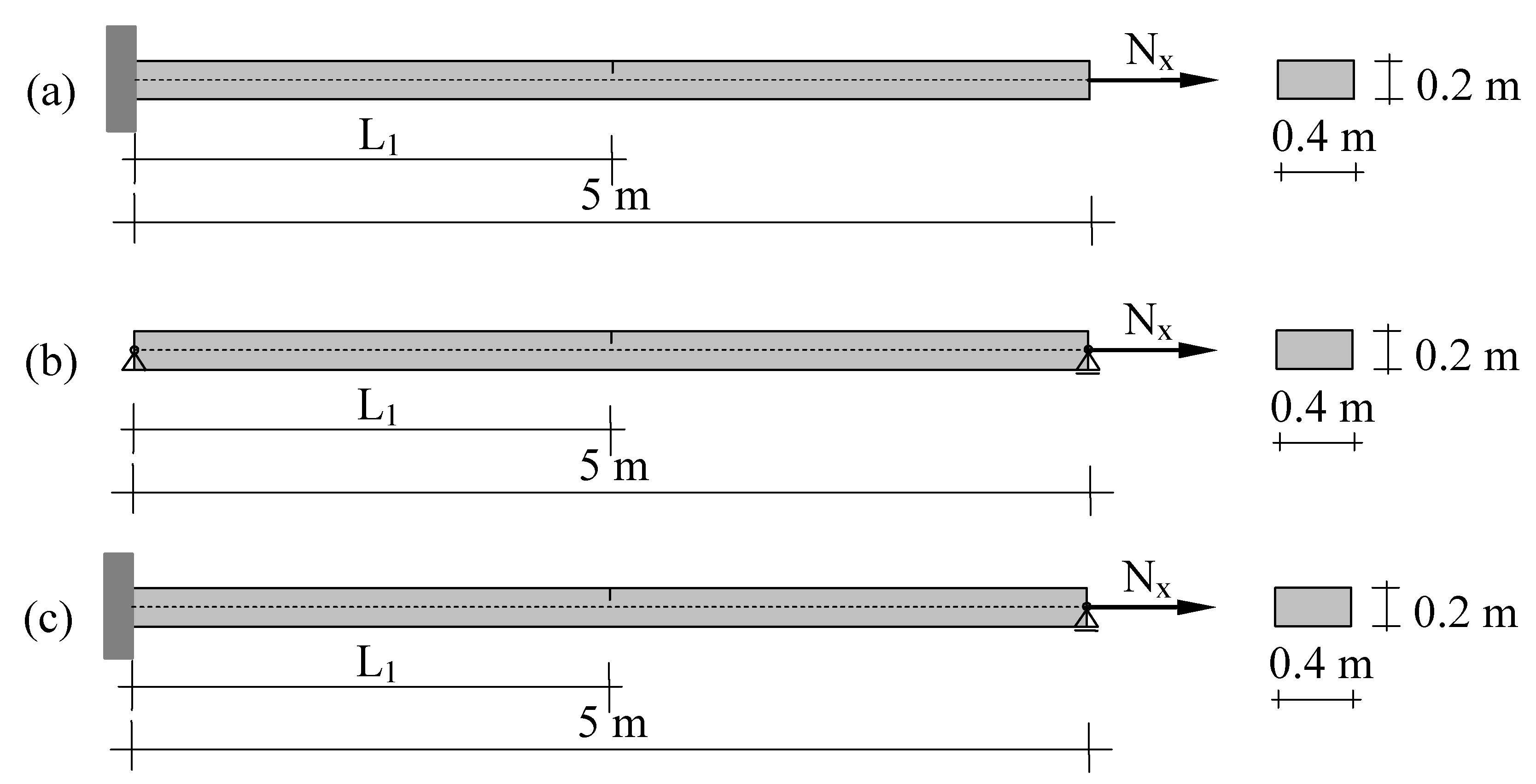
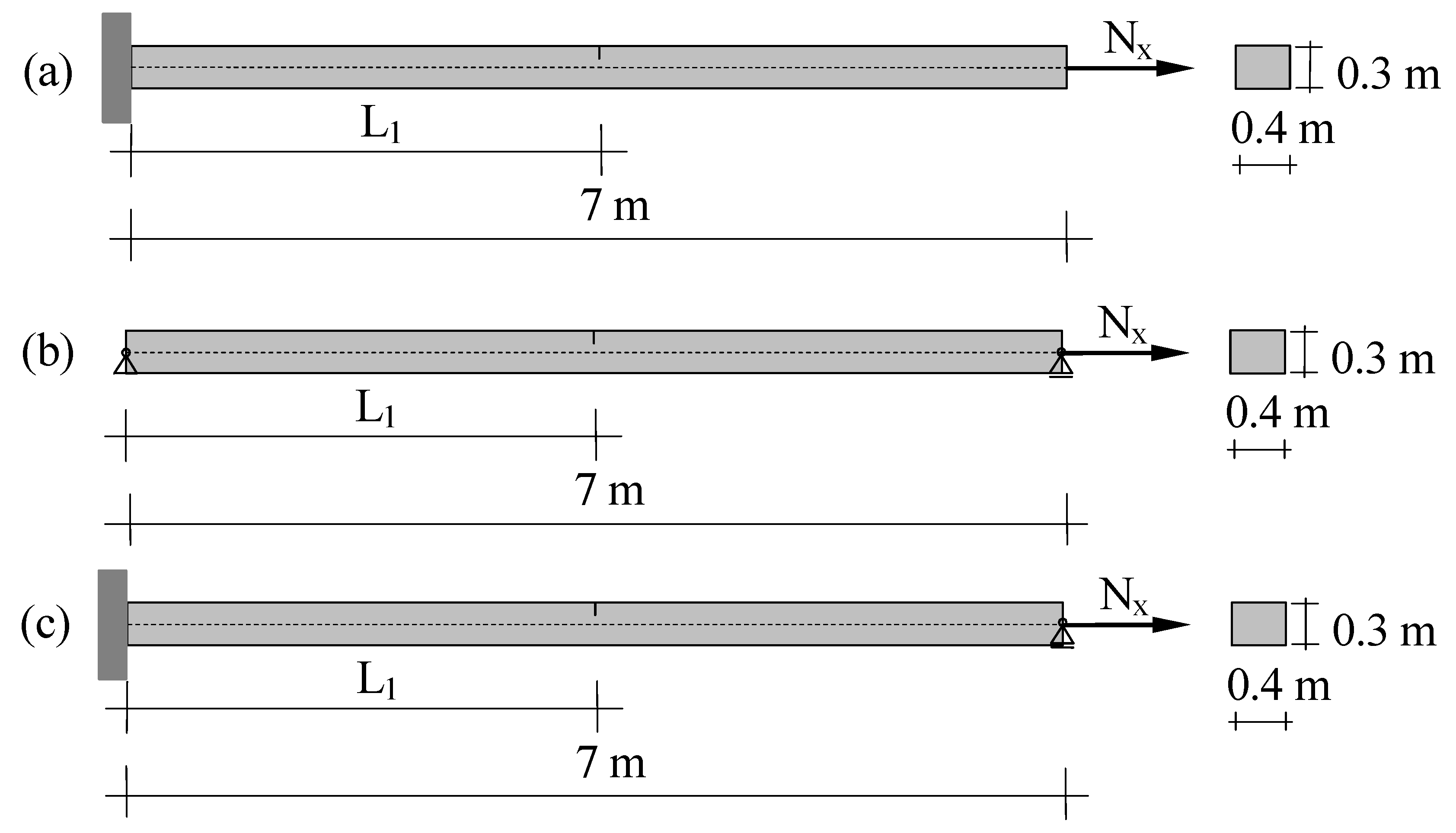
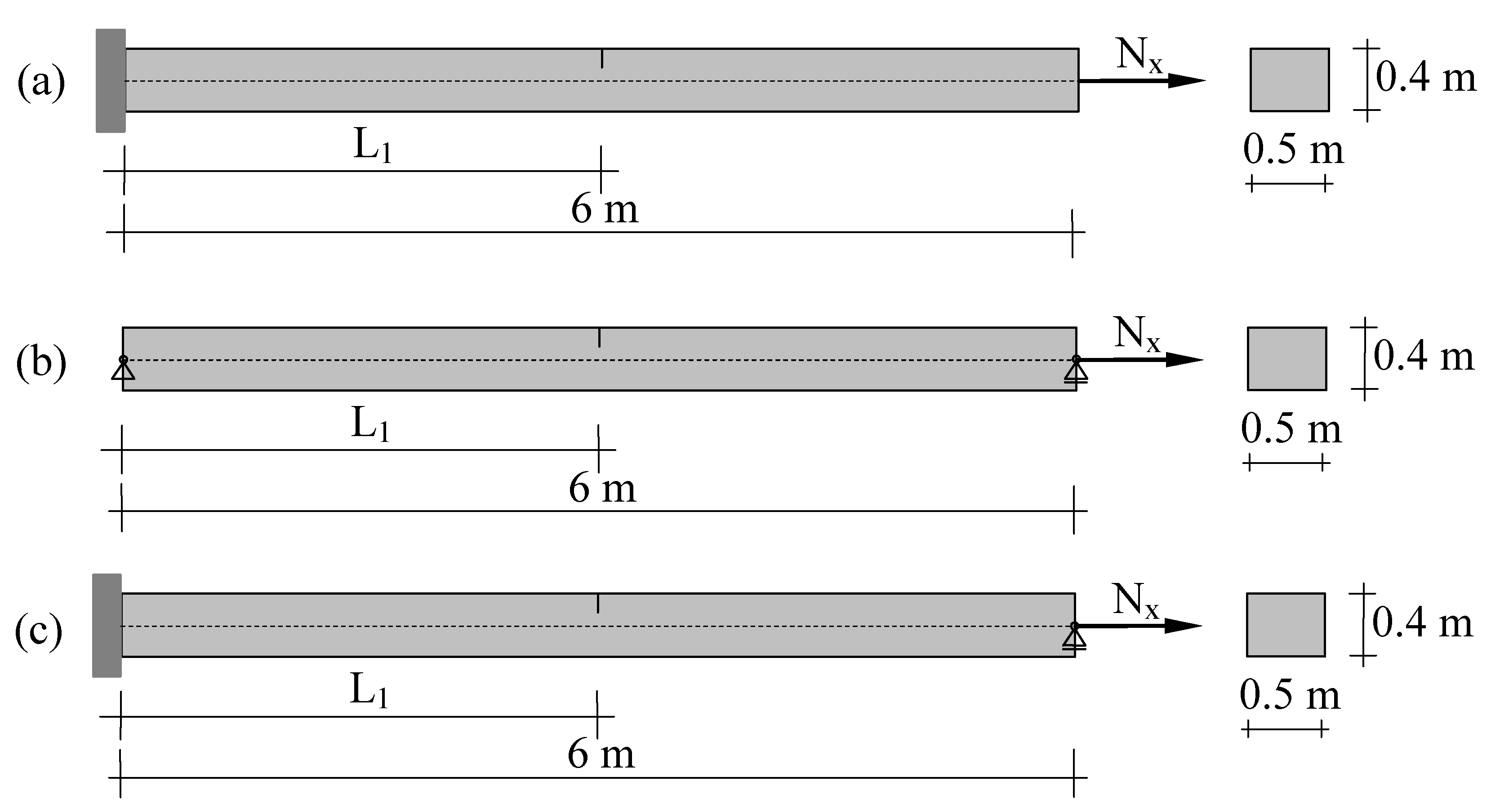
To begin with, three prismatic beams, B₁, B₂, and B₃, which differ in their geometric properties, were calculated in detail for different boundary conditions. For each type of beam, analyzes were performed with three different boundary conditions (cantilever clamped at the left end (C), simply supported beam (SS) and propped cantilever clamped at the left end (PC)). Geometric data of these beams (length L, width b and height h), together with the analyzed boundary conditions, are given in Figure 2, Figure 3 and Figure 4, representing nine basic (without detailed information on crack locations) combinations. 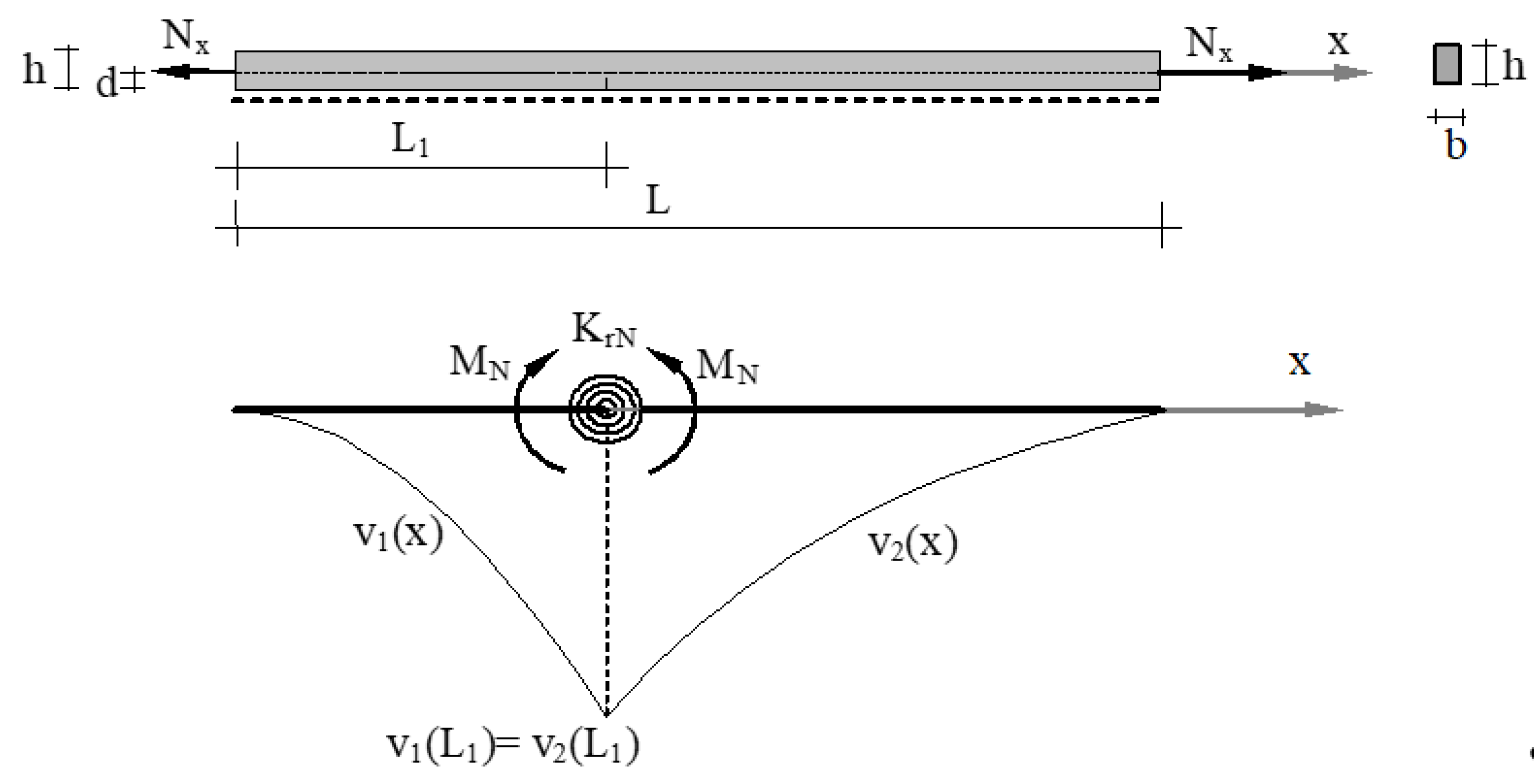The Young’s modulus E and the axial load N_x were 30 GPa and 1 MN, respectively. Furthermore, in each beam, transverse cracks were introduced individually at a distance of 0.5 m along each type of beam. At each location, six cracks of different depths were modeled. Relative depths between 0.1 and 0.6 were applied in steps of 0.1. Each crack was modeled on the upper surface of the beams, and as a result, its impact on the beam was reflected by a negative internal moment M_N.

Each 3D FE model consisted of 2000 elements in the axial direction, 30 in the vertical direction and 2 in the transverse horizontal direction. A total of 744 such models were analyzed (where almost 600,000 equations were solved in each analysis). The calculated vertical displacement at the crack point of each analyzed structure allowed the computation of the ratio ξ(δ) of the governing parameters of the model. The main results of each analysis were the vertical displacement at the crack location and the reactions in the supports (where they occurred). Ratio values for the same crack depths obtained for different locations were then compared to examine the effect of crack location on the identified ratio ξ(δ). The average results from all analyzed locations for each considered relative crack depth for beam type B₁ are given in

Table 1. Identified ξ(δ) ratios for the beam type B₁ (10⁻³) at different boundary conditions.

δ	B1C	B1C7	B1SS	B1SS6	B1PC
0.1	0.079012	0.078719	0.079359	0.079187	0.079344
0.2	0.357266	0.356543	0.357356	0.356992	0.358737
0.3	0.935136	0.933691	0.933412	0.932818	0.939049
0.4	2.038021	2.035238	2.032707	2.032876	2.046533
0.5	4.167478	4.161923	4.180188	4.173813	4.184832
0.6	8.573437	8.561219	8.586139	8.576524	8.609655

for cantilever clamped at the left end (B_1C), simply supported beam (B_1SS) and propped cantilever clamped at the left end (B_1PC). In the table, the results for the two additionally analyzed beams with modified lengths, a cantilever of 7 m length, B_1C7, and a simply supported beam of length 6 m, B_1SS6, are also included (they were analyzed only for initial testing of the hypothesis that beam length does not affect the identified values.).

The identified values of ξ(δ) were certainly not ideally the same for each relative depth δ, but their differences were clearly small enough to be easily attributed to the numerical modeling of the structure. Furthermore, since these values were identified at different crack locations L₁, their good agreement indicates that they depend solely on the relative depth of the crack δ and not on the location of the crack itself. Therefore, the identification process was repeated for beam type B₂, and the obtained average results for all three considered boundary conditions are presented in

Table 2. Identified ξ(δ) ratios for the beam type B₂ (10⁻³) at different boundary conditions.

δ	B2C	B2SS	B2PC
0.1	0.052996	0.053380	0.053119
0.2	0.240956	0.241424	0.241507
0.3	0.632549	0.631689	0.634021
0.4	1.379940	1.375981	1.383200
0.5	2.820635	2.820390	2.827522
0.6	5.793366	5.790182	5.806879

.

Although these values were not directly comparable to those from beam B₁ due to the different cross-sectional dimensions, they also showed good agreement for each relative crack depth δ analyzed.

Consequently, the analyses were also performed for beam type B₃, and the results for all three analyzed boundary conditions are presented in

Table 3. Identified ξ(δ) ratios for the beam type B₃ (10⁻³) at different boundary conditions.

δ	B3C	B3SS	B3PC
0.1	0.031932	0.032365	0.031999
0.2	0.145127	0.145776	0.145436
0.3	0.381025	0.380716	0.381835
0.4	0.831248	0.828609	0.832963
0.5	1.698993	1.694681	1.702461
0.6	3.489085	3.480894	3.495967

.

As with the previous beams, the average values of the three structures with different boundary conditions for each relative crack depth were in good agreement.

However, these values were again incomparable with the previously obtained ones due to the different cross-sectional dimensions of the analyzed beams.

Nevertheless, it can be reliably concluded from Table 1, Table 2 and Table 3 that the ratio ξ(δ) clearly depends on the relative depth of the crack δ, but at the same time it is independent of the location of the crack. Yet, in order to enable a direct comparison of the results for different cross-sections, it was necessary to convert the obtained ξ(δ) values to a common basis.

3.2. Conversion of Identified ξ(δ) Values into a Common Comparable Platform

In order to further compare the results for different cross-sections, Equation (4) was transformed into the following form in which the internal moment M_N in the numerator was defined by an upgraded definition compared to the simple definition given in Equation (1):

$$\xi \left(\delta \right)=\frac{\rho \left(\delta \right)·\delta ·h·N_x}{\frac{EI}{h·f_N\left(\delta \right)}}$$

(12)

For a rectangular cross-section, the expression takes form:

$$\xi \left(\delta \right)=\frac{12·\rho \left(\delta \right)·f_N\left(\delta \right)·\delta ·N_x}{EA}$$

(13)

where EA represents the axial stiffness of the beam.

By introducing a new dimensionless variable representing the normalized local slope change:

$$\overline{\xi }\left(\delta \right)=\rho \left(\delta \right)·f_N\left(\delta \right)·\delta$$

(14)

the following dimensionless relation can be obtained:

$$\overline{\xi }\left(\delta \right)=\frac{EA}{12·\delta ·N_x}·\xi \left(\delta \right)$$

(15)

which now allows a direct comparison of the obtained values for different cross-sections. Therefore, the values from Table 1, Table 2 and Table 3 were transformed accordingly to the common platform and are presented in

Table 4. (a). Identified $\overline{\xi }\left(\delta \right)$ ratios for the beam type B₁ at different boundary conditions. (b). Identified $\overline{\xi }\left(\delta \right)$ ratios for the beam type B₂ at different boundary conditions. (c). Identified $\overline{\xi }\left(\delta \right)$ ratios for the beam type B₃ at different boundary conditions.

(a)
δ	B1C	B1C7	B1SS	B1SS6	B1PC
0.1	0.015802	0.015744	0.015872	0.015837	0.015869
0.2	0.071453	0.071309	0.071471	0.071398	0.071747
0.3	0.187027	0.186738	0.186682	0.186564	0.187810
0.4	0.407604	0.407048	0.406541	0.406575	0.409307
0.5	0.833496	0.832384	0.836038	0.834763	0.836966
0.6	1.714687	1.712244	1.717228	1.715305	1.721931
(b)
	δ	B2C	B2SS	B2PC
	0.1	0.015899	0.016014	0.015936
	0.2	0.072287	0.072427	0.072452
	0.3	0.189765	0.189507	0.190206
	0.4	0.413982	0.412794	0.414960
	0.5	0.846191	0.846117	0.848256
	0.6	1.738010	1.737055	1.742064
(c)
	δ	B3C	B3SS	B3PC
	0.1	0.015966	0.016183	0.015999
	0.2	0.072563	0.072888	0.072718
	0.3	0.190513	0.190358	0.190917
	0.4	0.415624	0.414304	0.416481
	0.5	0.849496	0.847340	0.851231
	0.6	1.744542	1.740447	1.747983

. Table 4a–c show results for beam types B₁, B₂ and B₃, respectively.

It can be seen from all the tables that the calculated values for each relative depth δ now show a rational agreement.

Nevertheless, for better insight into the dispersion of the results from all obtained values for each relative crack depth δ, two extreme values (minimum value, ${\overline{\mathsf{\xi }}}_{min}$, and maximum value,${\overline{\mathsf{\xi }}}_{max}$) were identified from the 127 values calculated for each relative depth. Further, the mean ${\overline{\mathsf{\xi }}}_{mean}$ and median ${\overline{\mathsf{\xi }}}_{median}$ values as well as their ratios were also calculated for all relative crack depths,

Table 5. Extreme (min and max), mean, and median values for different relative crack depths.

δ	${\overline{\mathit{\xi }}}_{\mathit{m}\mathit{i}\mathit{n}}$	${\overline{\mathit{\xi }}}_{\mathit{m}\mathit{a}\mathit{x}}$	${\overline{\mathit{\xi }}}_{\mathit{m}\mathit{e}\mathit{a}\mathit{n}}$	${\overline{\mathit{\xi }}}_{\mathit{m}\mathit{e}\mathit{d}\mathit{i}\mathit{a}\mathit{n}}$	${\overline{\mathit{\xi }}}_{\frac{\mathit{m}\mathit{e}\mathit{a}\mathit{n}}{\mathit{m}\mathit{e}\mathit{d}\mathit{i}\mathit{a}\mathit{n}}}$	Δn (%)	Δp (%)
0.1	0.015744	0.016183	0.015920	0.015899	1.001346	−1.107	1.650
0.2	0.071309	0.072888	0.072064	0.072287	0.996929	−1.050	1.142
0.3	0.186564	0.190917	0.188735	0.189507	0.995928	−1.151	1.156
0.4	0.406541	0.416481	0.411384	0.412794	0.996583	−1.177	1.239
0.5	0.832385	0.851231	0.842025	0.846117	0.995164	−1.145	1.093
0.6	1.712244	1.747983	1.730136	1.737055	0.996017	−1.034	1.032

.

It can be seen from Table 5 that the mean and median values (columns 4 and 5) match almost perfectly, as their ratio (column 6) is almost equal to 1 for all relative crack depths. From the last two columns of Table 5, it is further evident that also the deviations of the extreme values from the mean values (Δ_n and Δ_p) are rather minor, as they do not exceed ±1.7%. 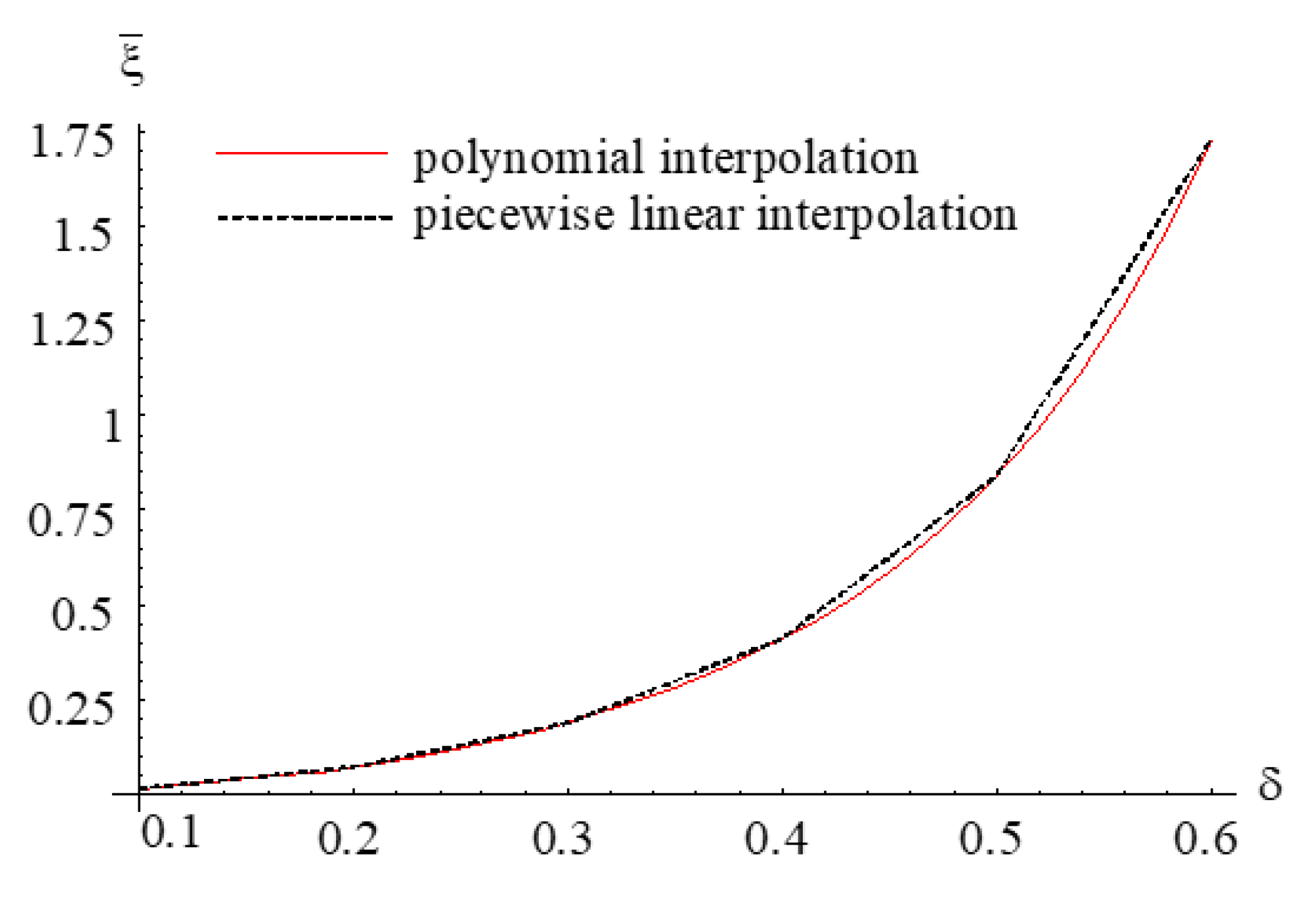Therefore, it is obvious that from an engineering point of view, the same $\overline{\xi }\left(\delta \right)$ function can be applied to different cross-sections. Its polynomial approximation is thus given as:

$$\overline{\xi }\left(\delta \right)=-0.0595+1.3840·\delta -10.3141·{\delta }^2+48.3954·{\delta }^3-90.0572·{\delta }^4+75.7498·{\delta }^5 0\le \delta \le 0.6$$

(16)

Figure 5 shows the piecewise linear approximation of the $\overline{\xi }\left(\delta \right)$ data (black dashed line) and the polynomial approximation derived by Equation (16) (red line).

3.3. Decoupling the Governing Parameters of the Model

As it became apparent that the same functions ρ(δ) and f_N(δ) could be used for different cross-sections, their separate evaluation was carried out. The research focus was on data on propped cantilevers, as it was clear from the displacement function of cantilever and simply supported beam (Equations (5)–(8)) that only the ratios ξ(δ) (but not separate individual functions) could be obtained. At first glance, the four parameters (displacement at the crack location, two vertical reactions, and a bending moment reaction) should allow direct calculation of both model parameters independently for each crack location L₁. However, basic equilibrium in the vertical direction requires that both vertical reactions be of equal magnitude (but in opposite directions), reducing the number of available parameters by one. Furthermore, the equilibrium of moments further implies that the reaction bending moment is equal to the vertical reaction multiplied by the length L of the beam, which further reduces the number of parameters by one. Therefore, the number of equations available for each crack location was reduced to two, which was still sufficient to determine the two discrete unknowns. The solution for the rotational spring stiffness K_rN from which the function f_N(δ) could be further found, was thus derived as:

$$K_{rN}=\frac{3·EI·{\left(L-L_1\right)}^2·V_B}{3·EI·\xi ·\left(L-L_1\right)-L^3·V_B}$$

(17)

and the corresponding value ρ(δ) could be further evaluated from Equation (4). Therefore, in the first attempt, the analysis for each crack location provided both discrete values using Equations (4) and (17) sequentially. The results for beam type B_1PC and relative crack depth of δ = 0.6 are given in the second and third columns of

Table 6. Identified discrete governing parameters K_rN and ρ for δ = 0.6 for propped cantilever B_1PC.

L1	KrN [×106]	ρ(δ)	$\overline{\mathit{\rho }}$(δ)
0.50	6.783186	0.488993	100.00%
1.00	6.760488	0.487357	99.665%
1.25	6.755733	0.487014	99.595%
1.50	6.749493	0.486564	99.503%
2.00	6.715160	0.484089	98.997%
2.50	6.660206	0.480128	98.187%
3.00	6.557508	0.472724	96.673%
3.50	6.345779	0.457461	93.552%
3.75	6.156856	0.443842	90.766%
4.00	5.832851	0.420484	85.990%
4.50	3.992671	0.287828	58.861%

(where the value of ξ = 8.650680 × 10⁻³ was used). The fourth column of the table presents the discrete values of the lever arm function normalized to the value at the first crack.

The last column of the table shows that the mutual matching of the results is quite good (the differences between the results are less than 1%) for the first third of the locations (i.e., up to the first third of the beam length from the clamped end). However, the increase in the discrepancies of the results becomes quite apparent as the crack location L₁ approaches the simply supported end. An even greater dispersion of results was evident for shallow cracks, where the zone with noticeable deviations extended further across the complete beam field.

Therefore, in the second attempt, only vertical reactions were used as input data for parameters identification. However, since only one vertical reaction cannot allow identification, vertical reactions from two arbitrary crack locations were used to obtain the two required values for each relative crack depth δ. Thus, each individual reaction was used multiple times, as it could be used in combination with all the remaining reactions for other crack locations of the same relative depth δ. In this way, combining the N_c crack data made it possible to obtain significantly more pairs of solutions than N_c.

Thus, the three considered propped cantilevers of beam types B₁, B₂ and B₃ and their crack locations (35 in overall) gave a total of 188 solution pairs (M_N, K_rN) for each crack depth δ considered.

The results exclusively for beam type B_1PC and a relative crack depth of 0.6 are given in

Table 7. All identified values of K_rN [×10⁶] for beam type B_1PC and a relative crack depth of 0.6.

6.810985	6.813096	6.815188	6.846570	6.853885
6.856316	6.858402	6.858680	6.862998	6.864356
6.865386	6.865491	6.865854	6.865937	6.866773
6.869885	6.870375	6.870738	6.871671	6.871884
6.872117	6.873537	6.873980	6.874276	6.874359
6.874731	6.875673	6.875929	6.876386	6.876517
6.877235	6.877882	6.878392	6.878433	6.878469
6.879129	6.879402	6.880205	6.880408	6.880548
6.880733	6.881666	6.882224	6.882327	6.882662
6.882918	6.884805	6.885264	6.885282	6.885317
6.885561	6.885844	6.900251	6.919794	6.926458

, where all 55 identified K_rN values are presented, ranked in ascending order.

The differences between the results are still noticeable. Nevertheless, a comparison of Table 7 and

Table 8. Identified values of the discrete lever arm ρ(δ) values from the three considered beams.

δ	Beam B1	Beam B2	Beam B3	Mean Value
0.6	0.493116	0.492707	0.492697	0.492831
0.5	0.530453	0.529120	0.529397	0.529623
0.4	0.597325	0.596270	0.596860	0.596784
0.3	0.722960	0.720536	0.720934	0.721418
0.2	1.004243	0.984961	0.982691	0.990277
0.1	1.812729	1.795792	1.859638	1.817743

shows that the dispersion of the results in Table 7 is evidently smaller as the deviations of the results from the mean value ranged from −0.902% to 0.778%. Similar, but even slightly smaller discrepancies of range −0.660% and 0.749% were detected for the values of the internal moment M_N. Thus, this approach to determining the two governing parameters not only provided a greater variety of results for K_rN and M_N, but also offered a more stable precision with a mean value that was very close to the median value.

Then, for each type of beam as well as for each relative crack depth δ, the discrete values of the normalized lever arms ρ(δ) were evaluated and further averaged. These values are presented in Table 8.

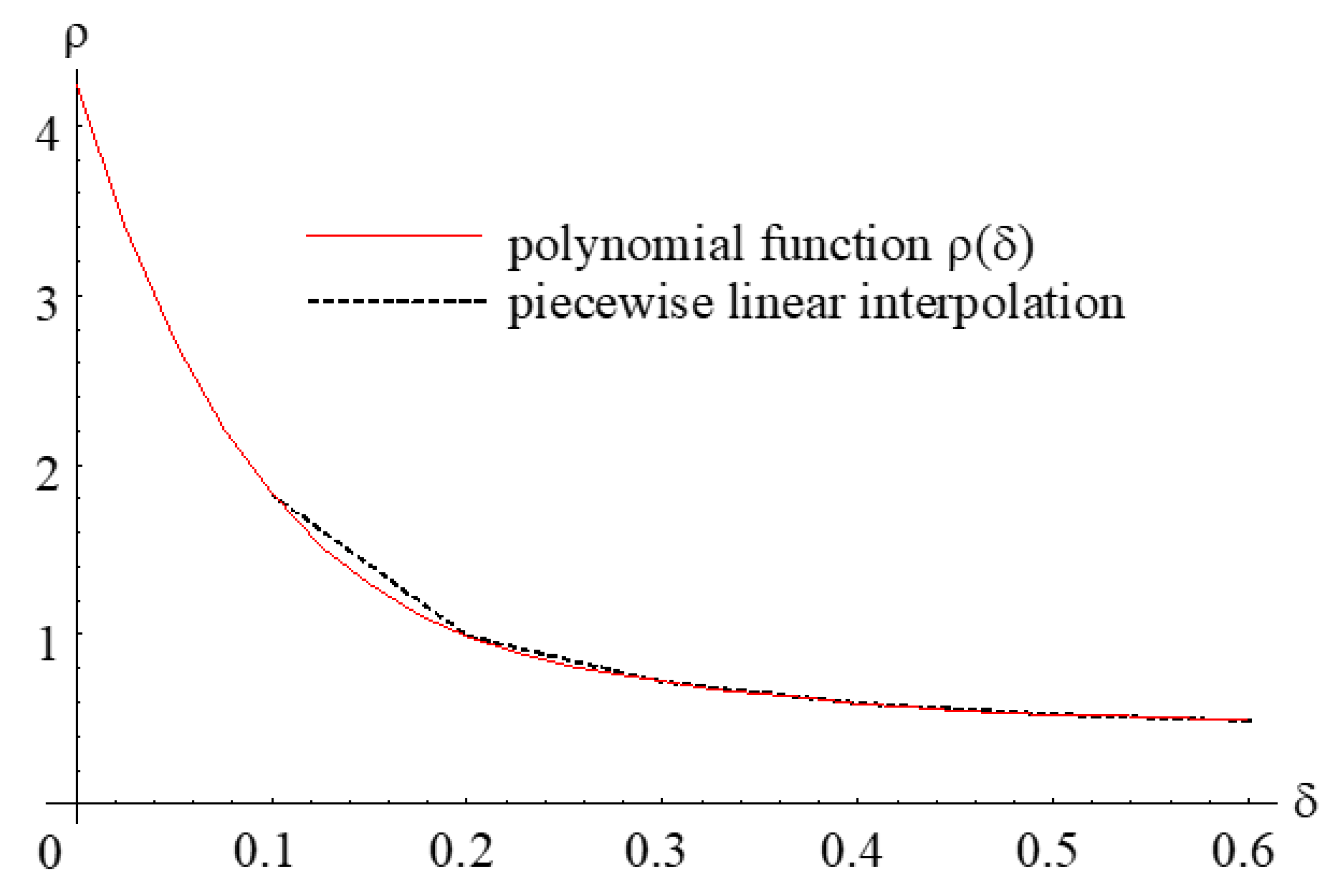
The weighted mean value for each relative crack depth δ was further used in an interpolation procedure to obtain a polynomial approximation function for ρ(δ).

$$\rho \left(\delta \right)=4.23-37.48·\delta +169·{\delta }^2-399.65·{\delta }^3+477·{\delta }^4-226·{\delta }^5\hspace{1em}0\le \delta \le 0.6$$

(18)

Figure 6, which proves the usefulness of the derived lever arm function, shows the piecewise linear interpolation of the original identified discrete values in the black dashed line, while the polynomial approximation function for ρ(δ) is plotted in the red line.

With the help of the known functions $\overline{\mathsf{\xi }}\left(\delta \right)$ and ρ(δ), it was further possible to calculate the missing function f_N(δ) from the definition of the stiffness K_rN of the rotational spring. The required function follows from Equation (14) in the form:

$$f_N\left(\delta \right)=\frac{\overline{\xi }\left(\delta \right)}{\rho \left(\delta \right)·\delta }$$

(19)

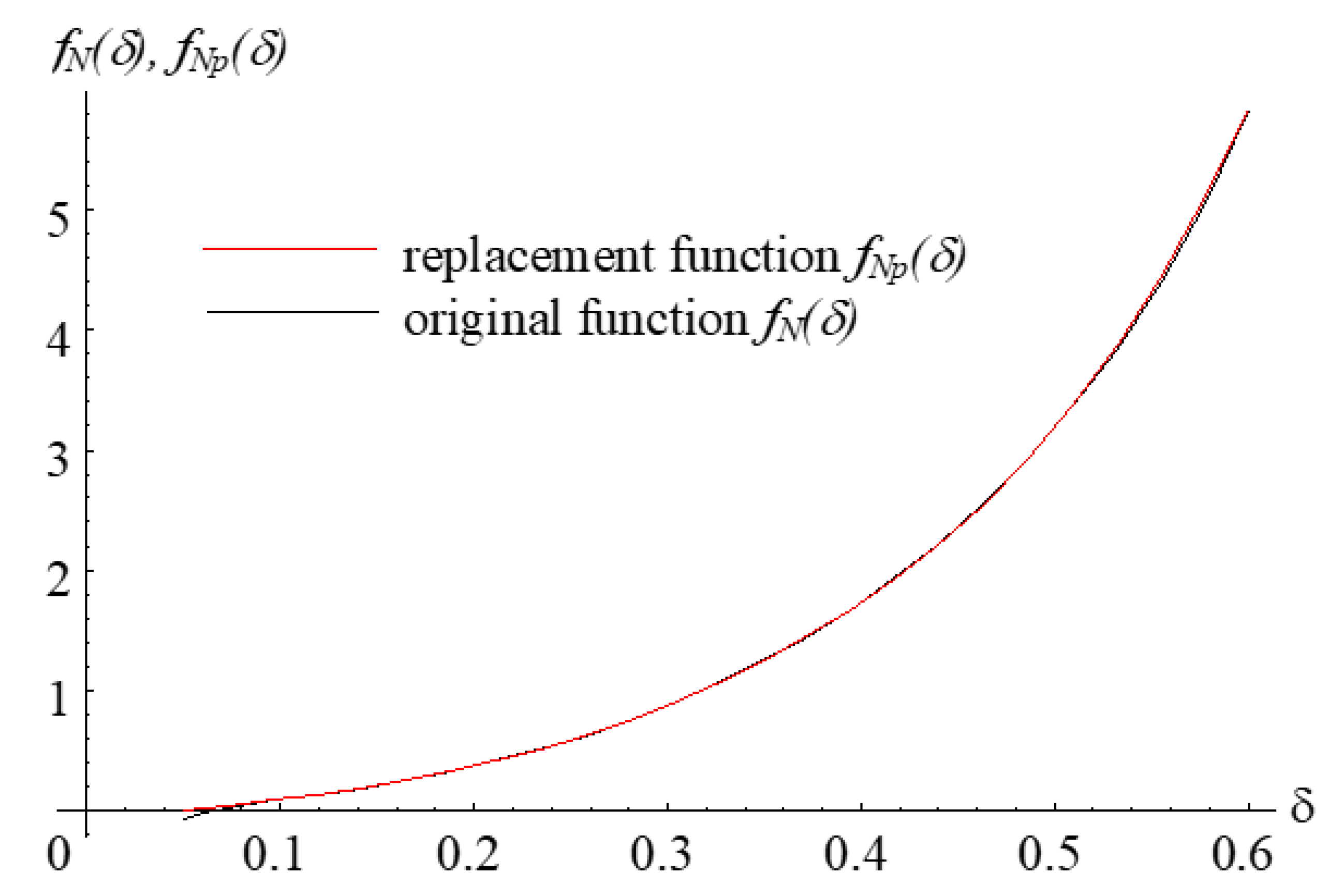
The original function f_N(δ) from Equation (19), initially given in the fractional form, was further replaced by a simple uniform polynomial function f_Np(δ) for practical reasons only. Figure 7 compares the graph of the original function f_N(δ) (black line) with its simple polynomial replacement f_Np(δ) (red line). From a comparison of the two graphs, it is evident that the match is generally more than decent, except in the area of very shallow cracks (i.e., δ < 0.1).

For the case without cracks, however, the rotational spring stiffness K_rN(δ) must be infinite, which consequently requires the function in the definition denominator to be zero. Therefore, in the derivation of the final function, a zero initial condition was additionally included, which resulted in a slightly modified function f_No(δ):

$$f_{N0}\left(\delta \right)=-0.127·\delta +11.414·{\delta }^2-22.026·{\delta }^3+95.961·{\delta }^4-171.221·{\delta }^5+159.754·{\delta }^6\hspace{1em}0\le \delta \le 0.6$$

(20)

4. Numerical Analyses

Initially, a comparison of transverse displacements for different locations L₁ and relative crack depths δ was performed. The results for a propped cantilever type B_1PC are presented in

Table 9. Comparison of the transverse displacement v_max (mm) for beam type B_1PC at the crack location from two different computational models.

L1	δ = 0.6	δ = 0.5	δ = 0.4	δ = 0.3	δ = 0.2	δ = 0.1
0.5	0.36372	0.21618	0.11027	0.054589	0.022581	0.005462
	0.35982	0.20985	0.11496	0.056763	0.022708	0.005150
1.0	1.32742	0.75590	0.39754	0.193685	0.077529	0.017843
	1.33697	0.75797	0.40690	0.198115	0.078519	0.017712
1.5	2.71323	1.49759	0.78035	0.375173	0.148242	0.033651
	2.73704	1.50835	0.79422	0.381725	0.150018	0.033677
2.0	4.27122	2.29104	1.17679	0.559159	0.218957	0.049336
	4.30889	2.30983	1.19458	0.567475	0.221363	0.049484
2.5	5.69986	2.97763	1.50736	0.708928	0.275653	0.061804
	5.74919	3.00273	1.52797	0.718451	0.278464	0.062025
3.0	6.66317	3.39999	1.69841	0.791934	0.306224	0.068420
	6.71934	3.42825	1.72026	0.801909	0.309161	0.068659
3.5	6.82179	3.41331	1.68575	0.780678	0.300636	0.067024
	6.87740	3.44046	1.70684	0.790200	0.303372	0.067219
4.0	5.87869	2.89870	1.41823	0.653561	0.251062	0.055937
	5.92371	2.91937	1.43619	0.661579	0.253226	0.056015
4.5	3.62936	1.77505	0.86037	0.395923	0.152495	0.034046
	3.65305	1.78355	0.87290	0.400879	0.153161	0.033847

. The first value (in regular) for each crack location/relative crack depth pair represents the displacement result (in mm) from the 3D model, and the second value (in italics) was obtained using a simplified model using the newly derived functions. Although it is evident that the directly comparable values are not identical, the matching of the results is completely fine from an engineering point of view, especially after considering the significant difference between the computational efforts of the two models.

In addition, Figure 8 shows in black lines the transverse displacement lines for beam B_1PC calculated by Equations (9) and (10) for relative crack depths δ from 0.1 to 0.6 and the crack located at the distance of 2 m from the left, clamped end. Both governing parameters of the model were calculated by implementing the presented solutions.

Further, these solutions are compared against the displacements from the 3D FE models, which are plotted as red dots in Figure 8. It is evident that a very good agreement has been obtained.

In the last step, the reactions on the supports (bending moment M_A and vertical reaction V_A in the left, clamped support, and vertical reaction V_B in the right, simple support) obtained from both models were compared. Accompanying values for beams whose displacement lines are presented in Figure 8 are given in

Table 10. Reactions for the beam type B_1PC.

δ	MA [Nm]	VA [N]	VB [N]
0.1	−227.9	−43.92	45.53
	−228.4	−45.68	45.68
0.2	−1017.2	−201.8	203.4
	−1021.7	−204.3	204.3
0.3	−2607.3	−517.4	521.4
	−2619.1	−523.8	523.8
0.4	−5488.8	−1095.6	1097.5
	−5513.5	−1102.7	1102.7
0.5	−10,607.4	−2120.0	2120.8
	−10,660.8	−2132.2	2132.2
0.6	−19,811.4	−3963.7	3963.0
	−19,887.2	−3977.4	3977.4

. The first value (in regular) for each relative crack depth δ represents the displacement result (in mm) from the 3D model, and the second value (in italics) was obtained by implementing a simplified model using the newly derived functions, Equations (18) and (20).

Despite the not-perfect agreement of the values from both computational models, the engineering matching of the results is evident. The average percentage error values for M_A, V_A, and V_B are 0.411%, 1.347%, and −0.437%, respectively. The slightly higher discrepancy value for the vertical reaction V_A is mainly influenced by the value −43.92 N (from the 3D FE model) for the shallowest crack, which also shows a visible discrepancy with the value of 45.53 N for the reaction V_B (from the same model). However, based on the equilibrium of moments, it can be concluded with certainty that V_A is a less accurate value than V_B.

5. Conclusions

In the article, the influence of the axial tensile force on the transverse displacements of slender prismatic beams with a single-sided crack was analyzed. A simplified model of a cracked beam was used to calculate transverse displacements and reactions. For this model, where the effect of the axial tensile force is modeled by an internal moment M_N acting at the crack location, improved governing parameters have been redefined based on extensive studies.

In the first step, many different beams were analyzed with 3D finite element models, which allow for accurate modeling of cracks. The study covered three different beams differing in geometrical properties, and for each beam type, analyses were made for different boundary conditions. For each analyzed combination of beam type and boundary conditions, transverse cracks were individually modeled at distances of 0.5 m along the entire length of each beam, and 6 cracks of different depths were modeled separately for each location.

Then, for each combination of boundary conditions, an analytical solution of the transverse displacement differential equation for the simplified cracked beam model was obtained. From the analytical expression for the transverse displacement at the crack location, the values of the ratio of the model’s governing parameters were obtained for all analyzed beams. These ratios depended on the associated geometrical data of the beam as well as the depth of the crack. However, after the transformation of the values to a common platform, it became evident that the ratio is truly independent of the beam geometry.

A new universal definition of the lever arm ρ(δ) as a function of relative crack depth δ was then derived. This definition replaced the rather basic definition from the initial studies and consequently allowed more realistic modeling of the internal moment M_N.

The rotational spring stiffness K_rN definition has also been updated to complete the improved model’s parameters.

The performed numerical tests showed that the model with improved definitions of its parameters can be effectively implemented for structural analyses through solutions of standard bending GDE without any axial force directly included in the governing differential equation. The presented expressions namely lead to reliable engineering results based on values from more thorough (and computationally more demanding) 3D FE models. These models initially served as a database generator and then also for independent verification.

However, although the discussed model represents an effective alternative to 3D FE models, it should be clearly noted that the presented solutions are limited to cracks with a relative crack depth value of up to 0.6.

References

1. Shifrin, E.I.; Ruotolo, R. Natural frequencies of a beam with an arbitrary number of cracks. J. Sound Vib. 1999, 222, 409–423. [Google Scholar] [CrossRef]
2. Khiem, N.T.; Lien, T.V. A simplified method for natural frequency analysis of a multiple cracked beam. J. Sound Vib. 2001, 245, 737–751. [Google Scholar] [CrossRef]
3. Li, Q.S. Free vibration analysis of non-uniform beams with an arbitrary number of cracks and concentrated masses. J. Sound Vib. 2002, 252, 509–525. [Google Scholar] [CrossRef]
4. Fernández-Sáez, J.; Navarro, C. Fundamental frequency of cracked beams in bending vibrations: An analytical approach. J. Sound Vib. 2002, 256, 17–31. [Google Scholar] [CrossRef]
5. Lin, H.P.; Chang, S.C. Forced responses of cracked cantilever beams subjected to a concentrated moving load. Int. J. Mech. Sci. 2006, 48, 1456–1463. [Google Scholar] [CrossRef]
6. Lee, S.; Jeong, M.; Cho, C.-S.; Park, J.; Kwon, S. Deep Learning-Based PC Member Crack Detection and Quality Inspection Support Technology for the Precise Construction of OSC Projects. Appl. Sci. 2022, 12, 9810. [Google Scholar] [CrossRef]
7. Feng, C.; Zhang, H.; Wang, H.; Wang, S.; Li, Y. Automatic Pixel-Level Crack Detection on Dam Surface Using Deep Convolutional Network. Sensors 2020, 20, 2069. [Google Scholar] [CrossRef] [Green Version]
8. Ali, L.; Alnajjar, F.; Jassmi, H.A.; Gocho, M.; Khan, W.; Serhani, M.A. Performance Evaluation of Deep CNN-Based Crack Detection and Localization Techniques for Concrete Structures. Sensors 2021, 21, 1688. [Google Scholar] [CrossRef]
9. Kim, I.-H.; Jeon, H.; Baek, S.-C.; Hong, W.-H.; Jung, H.-J. Application of Crack Identification Techniques for an Aging Concrete Bridge Inspection Using an Unmanned Aerial Vehicle. Sensors 2018, 18, 1881. [Google Scholar] [CrossRef] [Green Version]
10. Ren, J.; Zhao, G.; Ma, Y.; Zhao, D.; Liu, T.; Yan, J. Automatic Pavement Crack Detection Fusing Attention Mechanism. Electronics 2022, 11, 3622. [Google Scholar] [CrossRef]
11. Venugopal, A.; Mohammad, R.; Koslan, M.F.S.; Shafie, A.; Ali, A.b.; Eugene, O. Crack Growth Prediction on Critical Component for Structure Life Extension of Royal Malaysian Air Force (RMAF) Sukhoi Su-30MKM. Metals 2021, 11, 1453. [Google Scholar] [CrossRef]
12. Rodella, J.; Dhondt, G.; Köster, P.; Sander, M.; Piorun, S. Determination of the Crack Propagation Direction in Mixed-Mode Missions due to Cyclic Loading. Appl. Sci. 2021, 11, 1673. [Google Scholar] [CrossRef]
13. Hamishebahar, Y.; Guan, H.; So, S.; Jo, J. A Comprehensive Review of Deep Learning-Based Crack Detection Approaches. Appl. Sci. 2022, 12, 1374. [Google Scholar] [CrossRef]
14. Zhang, W.; Zhang, Z.; Qi, D.; Liu, Y. Automatic Crack Detection and Classification Method for Subway Tunnel Safety Monitoring. Sensors 2014, 14, 19307–19328. [Google Scholar] [CrossRef] [PubMed]
15. Munawar, H.S.; Hammad, A.W.A.; Haddad, A.; Soares, C.A.P.; Waller, S.T. Image-Based Crack Detection Methods: A Review. Infrastructures 2021, 6, 115. [Google Scholar] [CrossRef]
16. Golding, V.P.; Gharineiat, Z.; Munawar, H.S.; Ullah, F. Crack Detection in Concrete Structures Using Deep Learning. Sustainability 2022, 14, 8117. [Google Scholar] [CrossRef]
17. Chen, X.; Li, J.; Huang, S.; Cui, H.; Liu, P.; Sun, Q. An Automatic Concrete Crack-Detection Method Fusing Point Clouds and Images Based on Improved Otsu’s Algorithm. Sensors 2021, 21, 1581. [Google Scholar] [CrossRef]
18. Yang, C.; Chen, J.; Li, Z.; Huang, Y. Structural Crack Detection and Recognition Based on Deep Learning. Appl. Sci. 2021, 11, 2868. [Google Scholar] [CrossRef]
19. Hammouch, W.; Chouiekh, C.; Khaissidi, G.; Mrabti, M. Crack Detection and Classification in Moroccan Pavement Using Convolutional Neural Network. Infrastructures 2022, 7, 152. [Google Scholar] [CrossRef]
20. Teng, S.; Liu, Z.; Chen, G.; Cheng, L. Concrete Crack Detection Based on Well-Known Feature Extractor Model and the YOLO_v2 Network. Appl. Sci. 2021, 11, 813. [Google Scholar] [CrossRef]
21. Choi, D.; Bell, W.; Kim, D.; Kim, J. UAV-Driven Structural Crack Detection and Location Determination Using Convolutional Neural Networks. Sensors 2021, 21, 2650. [Google Scholar] [CrossRef] [PubMed]
22. Xu, X.; Zhao, M.; Shi, P.; Ren, R.; He, X.; Wei, X.; Yang, H. Crack Detection and Comparison Study Based on Faster R-CNN and Mask R-CNN. Sensors 2022, 22, 1215. [Google Scholar] [CrossRef]
23. Wang, B.; Li, Y.; Zhao, W.; Zhang, Z.; Zhang, Y.; Wang, Z. Effective Crack Damage Detection Using Multilayer Sparse Feature Representation and Incremental Extreme Learning Machine. Appl. Sci. 2019, 9, 614. [Google Scholar] [CrossRef] [Green Version]
24. Yan, J.; Downey, A.; Cancelli, A.; Laflamme, S.; Chen, A.; Li, J.; Ubertini, F. Concrete Crack Detection and Monitoring Using a Capacitive Dense Sensor Array. Sensors 2019, 19, 1843. [Google Scholar] [CrossRef] [PubMed] [Green Version]
25. Yankelevsky, D.Z.; Karinski, Y.S.; Feldgun, V.R. Analytical Modeling of Crack Widths and Cracking Loads in Structural RC Members. Infrastructures 2022, 7, 40. [Google Scholar] [CrossRef]
26. Huang, X.; Shi, C.; Ruan, H.; Zhang, Y.; Zhao, W. Stable Crack Propagation Model of Rock Based on Crack Strain. Energies 2022, 15, 1885. [Google Scholar] [CrossRef]
27. Smith, I.M.; Griffiths, D.V. Programming the Finite Element Method, 3rd ed.; John Wiley & Sons: Chichester, UK, 1997; pp. 21–27. [Google Scholar]
28. Reddy, J.N. An Introduction to the Finite Element Method, 2nd ed.; McGraw-Hill: Boston, MA, USA, 1993; pp. 143–154. [Google Scholar]
29. Skrinar, M. Elastic beam finite element with an arbitrary number of transverse cracks. Finite Elem. Anal. Des. 2009, 45, 181–189. [Google Scholar] [CrossRef]
30. Skrinar, M. Computational analysis of multi-stepped beams and beams with linearly-varying heights implementing closed-form finite element formulation for multi-cracked beam elements. Int. J. Solids Struct. 2013, 50, 2527–2541. [Google Scholar] [CrossRef] [Green Version]
31. Skrinar, M. Simple model for the vertical displacements computation of single cracked cantilever under tension loads. Z. Angew. Math. Mech. 2000, 80, 551–552. [Google Scholar] [CrossRef]
32. Skrinar, M. Transverse Displacements of Transversely Cracked Beams with a Linear Variation of Width Due to Axial Tensile Forces. In Engineering Design Applications III, 1st ed.; Öchsner, A., Altenbach, H., Eds.; Springer International Publishing: Cham, Switzerland, 2020; Volume 1, pp. 183–203. [Google Scholar]
33. Tauchert, T.R. Energy Principles in Structural Mechanics, 1st ed.; McGraw-Hill: Boston, MA, USA, 1974; p. 2. [Google Scholar]
34. Bowles, J. Foundation Analysis and Design, 5th ed.; McGraw-Hill: Boston, MA, USA, 1996; pp. 518–519. [Google Scholar]
35. Okamura, H.; Liu, H.W.; Chu, C.-S.; Liebowitz, H. A cracked column under compression. Eng. Fract. Mech. 1969, 1, 547–564. [Google Scholar] [CrossRef]
Figure 1. Transversely cracked tension beam and associated computational model.
Modelling 03 00031 g001
Figure 2. Tension beam B1 with different boundary conditions: (a) cantilever (B1C), (b) simply supported beam (B1SS), (c) propped cantilever (B1PC).
Modelling 03 00031 g002
Figure 3. Tension beam B2 with different boundary conditions: (a) cantilever (B2C), (b) simply supported beam (B2SS), (c) propped cantilever (B2PC).
Modelling 03 00031 g003
Figure 4. Tension beam B3 with different boundary conditions: (a) cantilever (B3C), (b) simply supported beam (B3SS), (c) propped cantilever (B3PC).
Modelling 03 00031 g004
Figure 5. Comparison of piecewise linear and polynomial approximation of ξ ¯ ( δ ) function.
Modelling 03 00031 g005
Figure 6. Piecewise linear interpolation and polynomial approximation of the ρ(δ) function.
Modelling 03 00031 g006
Figure 7. Comparison of functions fN(δ) and fNp(δ).
Modelling 03 00031 g007
Figure 8. Comparison of transverse displacements along the propped cantilever B1PC for various relative crack depths δ.
Modelling 03 00031 g008