Efficient Hydrodynamic Modelling of Urban Stormwater Systems for Real-Time Applications

Abstract

Urban water drainage systems represent complex networks with nonlinear dynamics and different types of interactions. This yields an involved modeling problem for which different off-line simulation approaches are available. Nevertheless, these approaches cannot be used for real-time simulations, i.e., running in parallel to weather now- and forecasts and enabling the monitoring and automatic control of urban water drainage systems. Alternative approaches, used commonly for automation purposes, involve parameterized linear delay systems, which can be used in real-time but lack the necessary level of detail, which, in particular, is required for adequate flood risk prognostics. Given this setup, in the present paper, an approach for the effective modeling of detailed water drainage systems for real-time applications implemented with the open-source Storm Water Management Model (SWMM) software is addressed and exemplified for a part of the water drainage system of the city of Flensburg in northern Germany. Additionally, a freely available early-warning system prototype is introduced and used to combine weather forcast information on a 2-h prediction horizon with the developed model and available measurements. This prototype is subsequently used for data assimilation using the ensemble Kalman filter (EnKF) for the considered area in Flensburg.

1. Introduction

Due to climate change, a shift in climatic behavior has been observed in recent years. In summer, long dry phases are followed by heavy rainfall events that bring large amounts of rain in a short period of time. In addition, persistent periods of rain can be observed in the winter months [1]. Since the capacities of urban stormwater networks in many cities are often not designed for these extreme situations, tools are needed to estimate the impact of upcoming rainfall scenarios in real-time [2]. In this way, precautionary actions can be taken before extreme events occur.

In the last decades, the term digital twin has become widespread with applications in many areas worldwide [3,4,5]. Based on a mathematical model of the system, the digital twin is supposed to provide insights into physical properties of the real plant and can support decision-making. The horizon of these decisions can range from everyday operations to long-term planning [6,7]. Prediction of extreme situations belongs to the area of everyday operations, since reliable weather forecasts are available only for a limited period of time [8]. For this operation mode, a model of the real plant must be developed that simulates its dynamic behavior accurately but sufficiently fast [7,9,10].

The modelling of stormwater systems has been investigated for decades and several different approaches have been presented [11,12,13,14]. In general, to accurately capture the behavior of the system both the channel system, which can be described by coupled one- or two-dimensional conduit components, and the surface flow have to be taken into account to investigate the distribution of the water on the surface in case of an overflow [15,16,17,18,19]. Both components can be described using combinations of 1D, 2D or 3D approaches, whereas the 3D approach is rarely used in practice due to heavy computational effort. Regarding the channel system, a 2D description can be useful if detailed information is required or if a big river is involved in the modelling area, but it is commonly modelled using connected 1D components. This typically leaves two combinations for practical use, namely the 1D1D and the 1D2D approach, where the surface is modelled in 1D and 2D, respectively. For both methods, the exact topology information of the surface is required and can be obtained from data of the geographical information system (GIS). They can be transformed to a surface grid on which the overland flow can be computed [11,20]. Rather detailed information can be obtained from 1D2D models [16,21]. However, three drawbacks have to be considered when using the 1D2D approach, which are the computational effort, the calibration effort and the potential license cost for commercial tools. From a computational point of view, the solution of the partial differential equations describing the shallow water flow is the most demanding component, especially when two dimensions are involved, and thus, the bottleneck with respect to real-time application [9,22]. Therefore, simplification methods for the 2D description and new modelling methods have been explored, and different approaches were presented in the last decades [11,15,18,23,24]. The 1D1D approach from [18] shows that 1D1D models can capture flooding reasonably well compared to the 1D2D model. For implementation purposes, a wide range of open-source and commercial tools have been developed [25]. Examples include the commonly used Storm Water Management Model (SWMM) from the US Environmental Protection Agency [26] and Mike Urban from DHI [27], which provides the possibility of 1D2D modelling.

The resulting models are based on the physical properties of the stormwater system and are typically called high-fidelity (HiFi) models, whereas surrogate models try to capture the dynamics based on a simplified or conceptual formulation of the network [10,28,29]. Many approaches for detailed and surrogate modelling have been proposed and compared in literature [28,29,30]. Surrogate models enable increasing the computational speed, which makes their use attractive for efficient simulation and real-time control [31,32,33,34,35]. However, since the flows of certain areas are usually combined, and the water level is only determined at some selected points in the system, the spatial accuracy is significantly reduced [10]. For that reason, the focus of this work points to the question of how efficient HiFi models can be used for real-time applications while maintaining the model accuracy.

Finally, to provide insights into the actual state of the real plant by a real-time monitoring system that can support decision-making, the unmeasured states have to be estimated, since only a few states are accessible through measurements. From a system-theoretic point of view, this problem is typically addressed using state-estimation or filtering techniques, such as the Kalman Filter with its different implementations [36,37]. In this approach, a particular form of data assimilation is employed in which the measurements are frequently compared to the simulation in real-time, and systematic corrections of the estimated states are performed to ensure minimum error covariance. Such data assimilation techniques have been introduced and applied to different types of urban stormwater systems (see, e.g., [38,39,40]), highlighting the great potential of these approaches for the problem at hand. Starting from an estimated state, future water levels and discharges of the system can be predicted based on the mathematical model in combination with the rainfall forecasts (cp., e.g., [39,41]).

In this article the efficient 1D1D modelling approach from [18] is further utilized, refined and transferred to the open-source tool SWMM. This approach is applied to obtain a model of the Mühlenstrom area in Flensburg (Germany), which is used as the case area of this work. An efficient model can be created automatically with the data handling structure presented in this paper. In addition, the real-time applicability of the resulting SWMM model is investigated, and a simulated real-time state estimation scheme is carried out using the ensemble Kalman filter (EnKF) as a data assimilation approach [37]. Since several simulations have to be run in parallel in this Monte-Carlo simulation-like scheme, the need for an efficient model is emphasized. Additionally, an open-source tool is presented that enables SWMM-based data assimilation and an early warning system for urban stormwater systems.

First, an approach for efficient modelling for urban stormwater systems is shown, whereupon the automatic data processing scheme is presented. After the considered data assimilation approach is briefly recalled, the open-source early warning tool is presented in Section 3. Thereupon, in Section 4, the results of the hydrodynamic modelling, the data assimilation and the flood forecasting system are shown. Finally, Section 5 concludes this paper with a summary and remarks for future investigations.

2. Hydrodynamic/Hydraulic Modelling

2.1. Description of the Channel Components

The simultaneously efficient and accurate modeling of a stormwater network on the city scale is a challenging task. To model such a system, many different components have to be taken into account, such as:

• Retention basins;
• Open and piped channels;
• Hydraulic structures;
• Catchments.

Retention basins enable storing a limited amount of water, which can be released later if a control actuator is available at the outlet. Their behavior follows the mass balance law

$$\begin{array}{c}\hfill \dot{V}=Q_{\mathrm{in}}-Q_{\mathrm{out}},V\left(t_0\right)=V_0\end{array}$$

(1)

of in- and outflow, which are denoted as $Q_{\mathrm{in}}$ and $Q_{\mathrm{out}}$, respectively. For practical implementation, the total volume V of the storage unit is derived from the water level and the topology of the basin.

Open and piped channels are the transport elements of the stormwater system, which connect catchment areas, retention basins and other elements of the system. In general, the mass balance and momentum equations should be taken into account to describe the flow of water. Inside the spatial domain $x\in (0,L)$ of length L, the wetted area A and the discharge Q at time $t>0$ can be described using the shallow water equations

$$\begin{array}{cc}\hfill \hspace{1em}\hspace{1em}\hspace{1em}\hspace{1em}\hspace{1em}\hspace{1em}\hspace{1em}\hspace{1em}\hspace{1em}\hspace{1em} {\partial }_{t}A+{\partial }_{z}Q=0,& \hfill A(z,0)=A_0,z\in [0,L],\end{array}$$

(2a)

$$\begin{array}{cc}\hfill {\partial }_{t}Q+{\partial }_z\left(\frac{Q^2}{A}\right)+gA({\partial }_{z}h+S_f-S_0)=0,& Q(z,0)=Q_0,z\in [0,L]\hfill \end{array}$$

(2b)

from St. Venant [42]. They give an accurate description of the channel flow and are commonly used in HiFi-models. The partial derivatives with respect to time and space are written as ${\partial }_t$ and ${\partial }_z$, while the water level, the gravitational acceleration, the bed and friction slope are denoted as h, g, $S_0$ and $S_f$, respectively. In addition, boundary conditions have to be set at the up- and downstream boundary, which are usually given by the wetted area or water level to ensure a spatially continuous water surface elevation. Since (Section 2.1) is a set of coupled hyperbolic partial differential equations, the time delay of the travel time is taken into account. The level of detail with regard to the network of conduits can be selected by setting a lower threshold on the pipe diameter, such that only such components are considered that have a sufficiently large diameter.

Hydraulic structures such as orifices, weirs and pumps have to be modelled individually based on their physical properties. The description of the individual hydraulic structures are given in [26]. These elements can be used to control the water flow if they can be actuated. Finally, catchments provide the input of precipitation to the hydrodynamic network. Available rain gauges are used to measure the current precipitation, while weather predictions can be obtained from radar data or numerical weather models. Radar data are more precise, while usually having a prediction horizon up to 2 h, whereas numerical models can be used to estimate future rain up to 10 or 14 days with decreasing accuracy over time. Based on the weather, now- and forecast future infiltration and runoff volumes can be calculated using approaches like the Green–Ampt model, Horton’s method or unit hydrographs. They define the inflow and thus the boundary conditions for the nodes in the model that are connected to catchment areas. For rivers that enter the modelling area, the boundary conditions are determined from the upstream area in combination with unit hydrographs to estimate the external inflow at those points.

2.2. Efficient Modelling of Surface Flows

When the water levels do not exceed the maximal storage of junctions and storages, the water will stay in the system, and the aforementioned components are sufficient to describe the system dynamics. However, in the real world, the water can exceed the limits of the channel system, which requires modeling the surface of the area as well. The rolling ball technique presented in [18] is briefly recalled and used to create a topology-based 1D1D mesh; it then computes the water levels and discharges on that mesh. This method aims to drastically reduce the computational time compared to the 2D surface modelling approach. The procedure basically consists of four steps. First, the surface is split into depression subareas based on the information of the surface elevation. This information can be obtained from the digital elevation model (DEM) data of the modelled area. Different thresholds can be set to ensure a minimal depth of the subareas. Thus, different mesh resolutions can be obtained. If detailed information is needed locally, a low threshold is recommended. Each of the identified subareas is assigned a storage with information about the maximal depth according to the head difference between the subarea boundaries and its deepest point. This point is subsequently called the subarea center point. Next, all interconnections of these subareas have to be modelled. For each depression area, the rolling ball technique is used to keep track of the contributing catchment area. Since the water can only leaves the storage if the physical boundary is exceeded, an overflow structure represents this process and connects the neighboring subareas. As the last step, the channel nodes—where the subareas could possibly drain to—have to be identified. Each of these connections are again modelled by using overflow structures. Depending on the terrain, the manholes are connected to a depression on the surface. The general idea of the overland flow simulation is illustrated in Figure 1.

The subareas are marked by the dashed gray circles, with the corresponding storage elements in darker green, which are able to exchange water between each other. Additionally, the storage elements can exchange water with open channels or manholes.

In total, a complex transformation from the 3D information of the DEM to an interconnected 1D surface model can be obtained. All data are stored in a database such that the pipe network and the 1D description of the terrain can be combined at any level of detail with respect to the included pipe dimensions and depression depths.

If the center points of two subareas are far away from each other, the travel time of the water should be taken into account. Therefore, additional conduit elements can be used, which again have to be connected by weirs at the border of the connecting subareas.

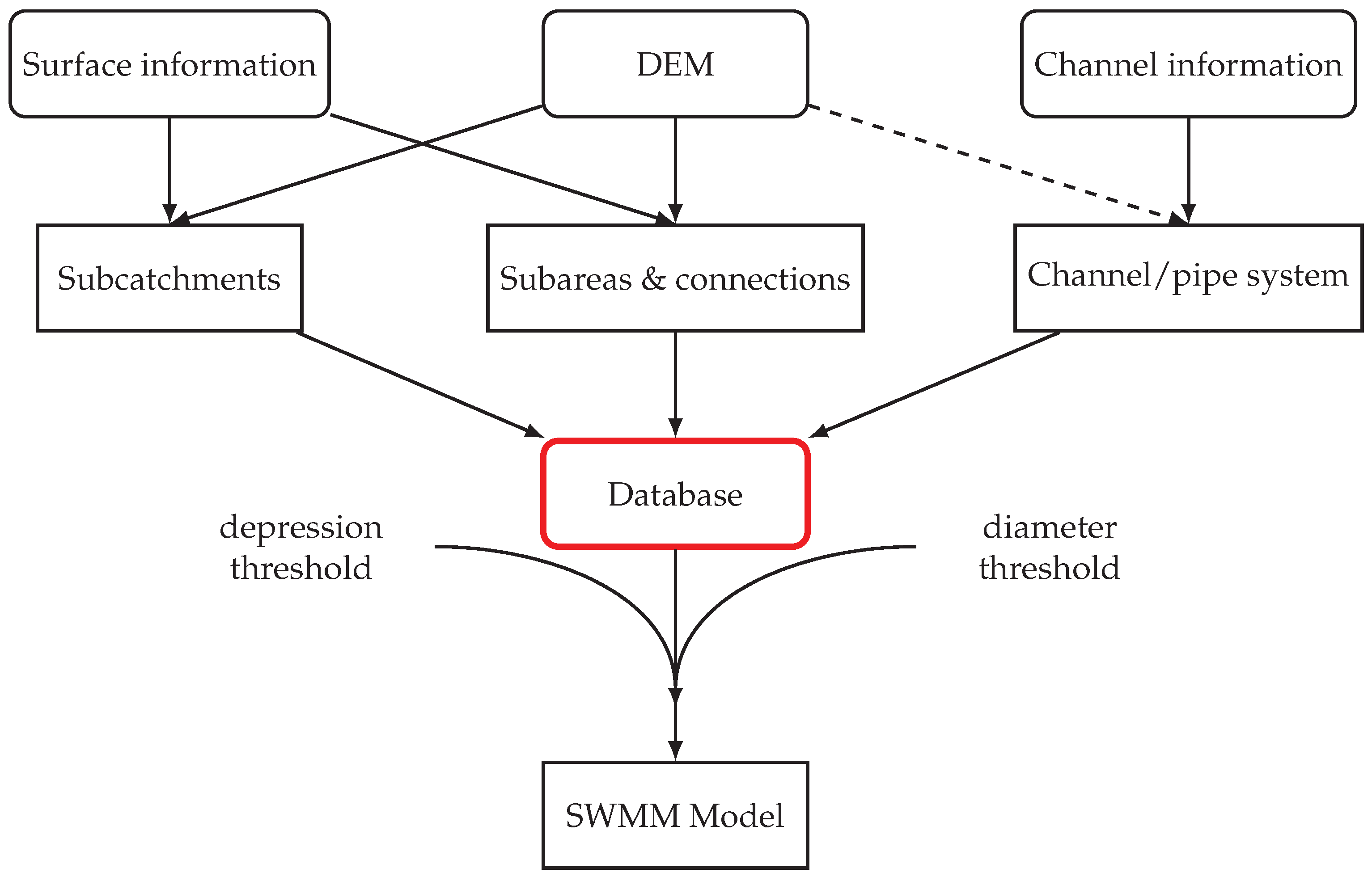
2.3. Data Processing

To set up the model automatically, different data sources have to be taken into account. The information about the channel system should include all storages and open and closed pipes with their corresponding parameters, e.g., their length, diameter and roughness. If these data are not complete, information from the DEM can help to identify channel pathways and storage areas. Additionally, available information about actuators such as gates, flow regulators and overflow structures have to be included to capture the behavior of the water system when the actuator settings are changed. All this information is typically available to the operators or maintainer of the system. To model the surface runoff in the catchments, information from the DEM is used to identify the dimension of a catchment, while its characteristics are obtained from the surface material composition. If this information is not available, it can be approximated using satellite pictures, e.g., from Google Maps. From the DEM model, all depression subareas with a minimal depth of 10 cm and all connecting links are identified and added to the database. The parameters to describe the overflow structure and the dimensions (area-depth curve) of the depression are given in the DEM, whereas the infiltration to the soil has to be obtained from the surface material again. For each component, a separate entry in the database is created, while other type-dependent databases store the corresponding parameters of the system elements.

Finally, to create the SWMM model, the channel diameter and depression thresholds are chosen, and the model is created sequentially. First, information about the channel system is set up. Therefore, all channels that satisfy the threshold condition are modelled as conduits, whereas the connecting nodes are modelled as junctions or storages, depending on the node type. Additional junctions are included if a subcatchment drains to a point in the channel. The subcatchments are directly transferred to the SWMM model with the parameters from the database. To conclude the channel system model, the control actuators are included. Subsequently, the surface depressions are modelled as storages with the corresponding area-depth curve from the database. All connections between the considered depression subareas are taken from the database, and the overflow structures are modelled as weir elements in SWMM. A schematic overview of the data processing scheme for the automatic creation of efficient 1D1D SWMM models is given in Figure 2.

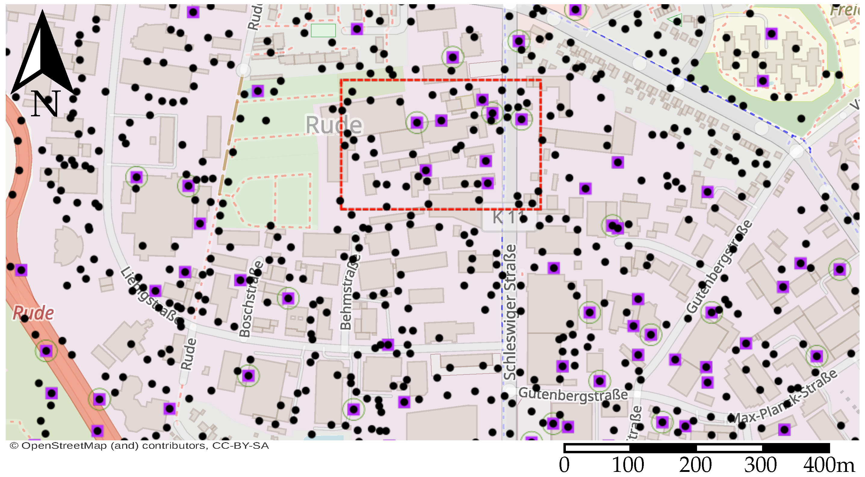
2.4. Application of Stormwater System Modelling in Flensburg

2.4.1. Characteristics of the Case Study Area

Flensburg is a city in northern Germany (at 54${}^{\circ }$47${}^{\prime }$ N, 9${}^{\circ }$26${}^{\prime }$ E) close to the border of Denmark with approximately 90.000 inhabitants. The city center is located at the Baltic Sea (1 m above sea level), while the foreland lies on a plateau about 50 m above sea level. However, this difference in altitude is covered within a distance of about 4 km, which results in steep slopes in some areas. These already belong to an urbanized area with residential and industrial parts. The total catchment area of the considered case area is about 6.000 hectares, whose water is drained to the Baltic Sea through open and closed underground channels, with a total length of approx. 229 km. Five larger natural retention basins with a total volume of approx. 260.000 m${}^3$ can be used to store water temporarily. The response time of the system is around two hours.

2.4.2. Developement of the SWMM Model

Based on the channel information, which has been provided by the utility, the hydraulic components of the pipes, including manholes, were transferred to the database. All controllable actuators were identified, whereas the information about the open retention basins was extracted from the DEM and subsequently converted to area-height curves to describe the storage capacity of the natural basins. Fortunately, a detailed mapping of the surface was made by the utility for maintenance, which simplified the identification of the surface imperviousness. By using information from the DEM, the database entries for subcatchments and surface subarea center points, including their pathways, were subsequently added.

Different levels of detail can be obtained depending on the threshold setting for the pipe diameter. It is also related to the computational effort that is needed to simulate the system. In this work, all pipes with a diameter bigger than 30 cm have been taken into account. This results in a channel system model of the case area, which is displayed in Figure 3. The urban sub-catchment areas are colored, while the open and closed channels are marked in blue.

Regarding the surface network, different depression thresholds will be considered and analyzed later in this work. Figure 4 shows the identified subarea center points with the corresponding depression depth.

The subareas and the corresponding subarea center points from the window marked in Figure 4 are displayed in Figure 5a. Additionally, all interconnecting overflow structures between neighboring subareas are sketched in Figure 5b.

Finally, a SWMM modell with 1078 junction, 18 storage, 1110 conduit and 5603 catchment elements in total is obtained for the channel system with a minimal pipe diameter of 30 cm. When the surface flow is modelled, 718 storages and 2787 weir elements are added for the Mühlenstrom area when a depression threshold of 30 cm is chosen.

3. Data Assimilation

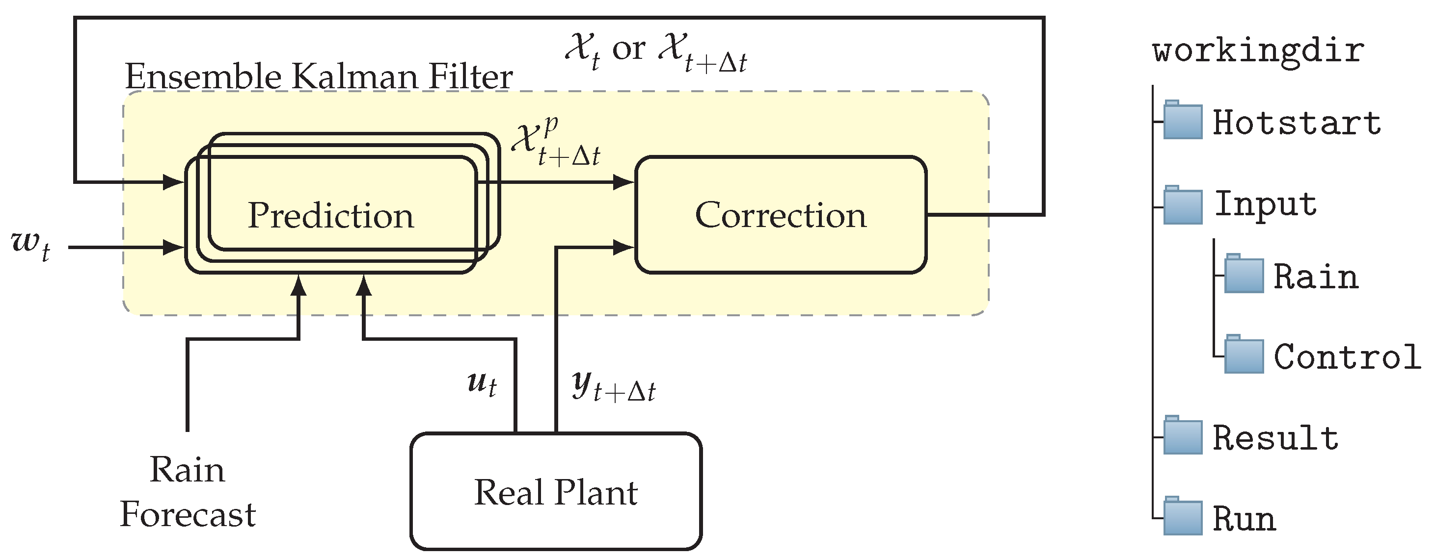
3.1. General Idea

The mathematical model tries to capture the dynamics of the stormwater system. However, two things must be taken into account if the model is to be used for monitoring and as an early warning system of the real stormwater network. Even after sufficient calibration and detailed modelling using extensive information of sub-catchments and the hydraulic structures, the model will never capture the behavior of the real world exactly [43]. Furthermore, different behaviors will be predicted even when the model is quite exact but the initial conditions are not correct. In order to be able to simulate and predict the behavior of the real world starting from an estimated initial state, it is thus necessary to use available measurements for automatic comparison with the simulation. This can be achieved by an adequate data assimilation scheme. Different data assimilation techniques have been proposed in the literature.

A classical approach is the Kalman filter [36] or a modified version, whose scheme can be divided into two steps. First, the estimated state ${\widehat{\mathit{x}}}_t^{}$ at time t is propagated over a time interval $\Delta t$ using an internal model ${\mathcal{M}}_i$ to obtain a predicted state

$$\begin{array}{c}\hfill {\widehat{\mathit{x}}}_{t+\Delta t}^p={\mathcal{M}}_i\left(\begin{array}{c}\hfill {\widehat{\mathit{x}}}_t^{}+{\mathit{w}}_t^{},{\mathit{u}}_t\end{array}\right),{\mathit{w}}_t^{}\sim \mathcal{N}\left(0,Q_t\right),\end{array}$$

(3)

which is disturbed due to process noise (e.g., model inaccuracies), with covariance $Q_t$; it depends on the control input, which is denoted as ${\mathit{u}}_t$. Thereupon, when the measurement ${\mathit{y}}_{t+\Delta t}$ is available, the estimated states can be updated using

$$\begin{array}{c}\hfill {\widehat{\mathit{x}}}_{t+\Delta t}^{}={\widehat{\mathit{x}}}_{t+\Delta t}^p+K({\mathit{y}}_{t+\Delta t}-{\widehat{\mathit{y}}}_{t+\Delta t}^p),\end{array}$$

(4)

where ${\widehat{\mathit{y}}}_{t+\Delta t}^p=H{\widehat{\mathit{x}}}_{t+\Delta t}^p$ denotes the simulated output, i.e., the level and/or flow value measurements at specific points. In general, the Kalman correction gain

$$\begin{array}{c}\hfill K=P^p{H}^T{\left(H^T{P}^{p}H+R\right)}^{-1},\end{array}$$

(5)

for which a minimum error covariance is ensured under some assumptions [36,37,44,45] can be determined using the predicted covariance $P^p$ of the estimation error, which depends explicitly on the measurement noise covariance R. Different approaches can applied to obtain $P^p$. In contrast to the classical and extended Kalman filter [36], where a Riccati equation must be solved at each time step to determine the covariance matrix of the predicted state, the EnKF determines the covariance using ensembles. Since the computational effort increases quadratically with the number of states when solving the Riccati equation, the EnKF is rather suitable for high-dimensional systems. Additionally, the EnKF is a preferred choice when the underlying system dynamics are nonlinear [44,45]. The general idea of the EnKF is to propagate an ensemble

$$\begin{array}{c}\hfill {\mathcal{X}}_t^{}=\left[\begin{array}{ccccc}{\widehat{\mathit{x}}}_t^1& \cdots & {\widehat{\mathit{x}}}_t^i& \cdots & {\widehat{\mathit{x}}}_t^N\end{array}\right]\end{array}$$

(6)

with N members of estimated states using the system dynamics ${\mathcal{M}}_i$. The predicted states of the ensemble ${\mathcal{X}}_{t+\Delta t}^p$ are corrected by using the deterministic update step. Here, the approach introduced in [37] is used for this purpose, as it appears to be more robust compared to, e.g., using an update step involving artificial measurement noise injection. First, the predicted mean

$$\begin{array}{c}\hfill {\overline{\mathcal{X}}}_{t+\Delta t}^p=\frac{1}{N}\sum _{i=1}^N{\widehat{\mathit{x}}}_{t+\Delta t}^{i,p}\end{array}$$

(7)

is calculated from the predicted ensemble members ${\widehat{\mathit{x}}}_{t+\Delta t}^{i,p}$. This ensemble mean is updated as described in (4) to obtain ${\overline{\mathcal{X}}}_{t+\Delta t}^{}$. Therefore, the Kalman gain is computed from (5) using the relationships

$$\begin{array}{c}\hfill H^T{P}^{p}H=P_{y,y}=\frac{1}{N-1}\sum _{i=1}^N(H{\mathcal{X}}_{t+\Delta t}^p-H{\overline{\mathcal{X}}}_{t+\Delta t}^p){(H{\mathcal{X}}_{t+\Delta t}^p-H{\overline{\mathcal{X}}}_{t+\Delta t}^p)}^T\end{array}$$

(8)

and

$$\begin{array}{c}\hfill P^p{H}^T=P_{x,y}=\frac{1}{N-1}\sum _{i=1}^N({\mathcal{X}}_{t+\Delta t}^p-{\overline{\mathcal{X}}}_{t+\Delta t}^p){(H{\mathcal{X}}_{t+\Delta t}^p-H{\overline{\mathcal{X}}}_{t+\Delta t}^p)}^T.\end{array}$$

(9)

Subsequently, to update all ensemble members, the predicted ensemble anomaly

$$\begin{array}{c}\hfill {\mathcal{A}}_{t+\Delta t}^p=\left[\begin{array}{ccccc}{\widehat{\mathit{x}}}_{t+\Delta t}^{1,p}-{\overline{\mathcal{X}}}_{t+\Delta t}^p& \cdots & {\widehat{\mathit{x}}}_{t+\Delta t}^{i,p}-{\overline{\mathcal{X}}}_{t+\Delta t}^p& \cdots & {\widehat{\mathit{x}}}_{t+\Delta t}^{N,p}-{\overline{\mathcal{X}}}_{t+\Delta t}^p\end{array}\right]\end{array}$$

(10)

is computed and updated using

$$\begin{array}{c}\hfill {\mathcal{A}}_{t+\Delta t}^{}={\mathcal{A}}_{t+\Delta t}^p+\frac{1}{2}KH{\mathcal{A}}_{t+\Delta t}^p.\end{array}$$

(11)

Finally, the updated ensemble is given by

$$\begin{array}{c}\hfill {\mathcal{X}}_{t+\Delta t}^{}={\mathcal{A}}_{t+\Delta t}^{}+\left[\begin{array}{ccc}{\overline{\mathcal{X}}}_{t+\Delta t}^{}& \cdots & {\overline{\mathcal{X}}}_{t+\Delta t}^{}\end{array}\right].\end{array}$$

(12)

The scheme is applied iteratively with time intervals of $\Delta t$ to assimilate the measurement data and thus compensate for initial value errors in ${\mathcal{X}}_{t_0}^{}$, model uncertainties (as far as possible) and keep track of the real states. Starting from the adapted actual estimate ${\mathcal{X}}_{t+\Delta t}^{}$, the model can be used to simulate beyond the prediction horizon of $\Delta t$, which offers the possibility to use it as an early warning system. Since the measured quantities are directly simulated within the model, the output matrix H is linear. Otherwise, a linearization could be used.

To obtain information about which states can be adequately estimated in a fixed time interval, an observability analysis of the developed model has to be carried out based on the given sensor configuration [46]. Typically, large systems are analyzed for their structural observability [47], which is a necessary condition to be fulfilled if the system should be observable. Applying the graph-based approach on the 1D1D stormwater system yields, the structural observability is lost when there is no exchange between neighboring subareas or with the conduit system. Since this is the case most of the time, the internal model that is used for state estimation was chosen to contain only information about the channel system in the present study. Accordingly, all states from the channel system are estimated from the available sensor information using the data assimilation scheme. In

Table 1. Components of the estimated state.

Component Type	Depth	(In-)Flow	Runoff
Storages	×	×
Nodes	×	×
Links	×	×
Subcatchments			×

, the information which is available from the estimated states is summarized. Further information could be obtained from the ensemble SWMM simulation.

3.2. Implementation in Forecasting System

As proposed in the introduction, a python-based open-source tool is introduced that can be used for data assimilation and forecasting hydrodynamic systems when an underlying SWMM model is available. The scheme of the data assimilation process and the folder structure that is used in the tool is sketched in Figure 6.

In general, when using SWMM for prediction purposes, the states can be initialized through a so-called hot-start file, which is automatically read in from SWMM when a simulation is started.

When starting the process for the first time, an initial guess ${\mathcal{X}}_{t_0}^{}$ is created for each of the N ensemble members using uniformly distributed water levels from zero to its maximal water depth for all nodes, storages, and links. The information about the maximal water depth of these states is obtained from the underlying SWMM model, which is read in using the swmm-api toolkit [48]. Inflows are initialized by zero values. The initial conditions of all ensembles are stored in individual hot-start files in the Hotstart folder, and a corresponding SWMM model is stored in the Run folder, where it is executed by the python wrapper pyswmm [49]. Expected rain time series and future control settings are stored in the Input folder. Finally, the prediction results are stored in the Results folder. Regarding the rain forecast, these data can be extracted from radar data by converting the raw data to an ensemble of time series on a $1\times 1$ km grid. However, this part is not included in the tool since the data source format usually varies. Thus, the SWMM models of all ensemble members can be run in parallel with different combinations of initial conditions and possible rainfall events. After executing the parallel simulations over the prediction horizon, a hot-start file for each ensemble is created that contains the predicted states. When the measurements are available, those hot-start files are read in, and the previously described data assimilation scheme is carried out to obtain the corrected states ${\widehat{\mathit{x}}}_{t+\Delta t}^i$. They are used to rewrite the hot-start files before the next forecasting step is started. To speed up the simulations, SWMM uses openMP parallelization, which results in significantly reduced simulation time [50]. In addition, all instances of the forecasting system are run in parallel in the CPU to minimize the computational time needed for one iteration.

All measurements and forecasts are displayed on a graphical user interface, where different nodes and links can be selected to be displayed as a plot or on an interactive map (if coordinates are available). Additionally, if there is no access to the real plant, a model that simulatively represents the system can be used instead.

4. Results

In this section, first the results and accuracy of the efficient 1D1D modeling approach are examined before the ensemble-based system monitoring and prediction scheme are evaluated in the simulation of the case area Mühlenstrom in Flensburg.

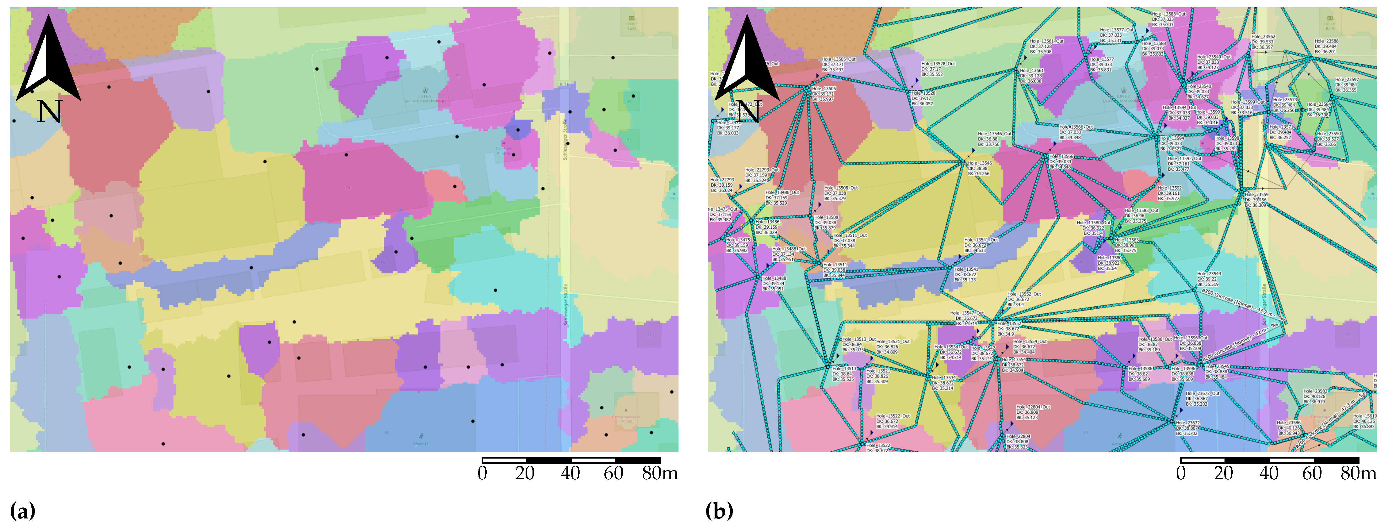
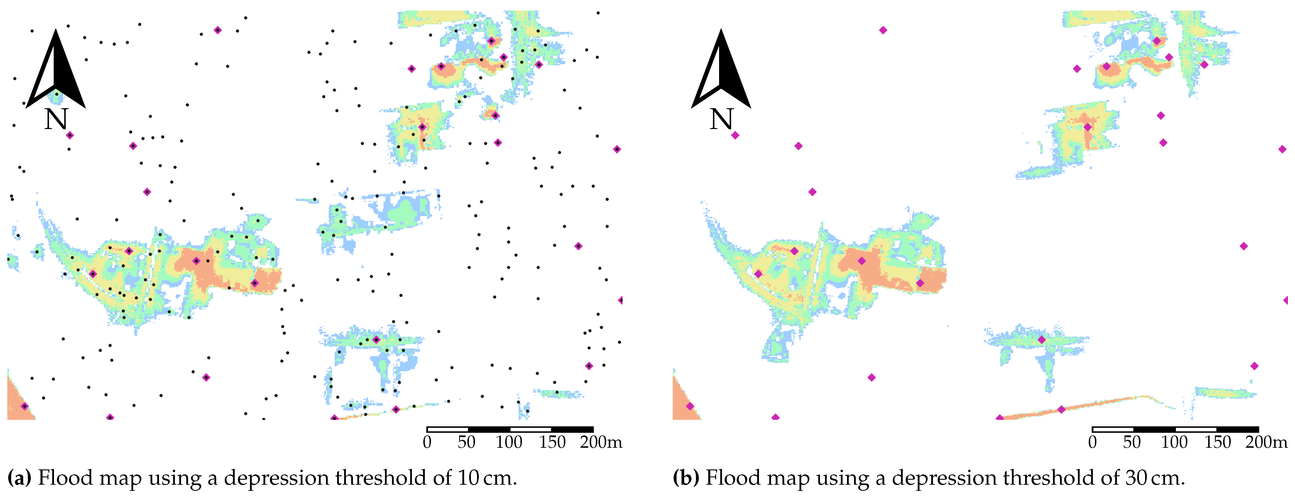
4.1. Results of 1D1D Surface Modeling

To evaluate the matching between the model and historic data, a rain event from April 2022 was selected. The precipitation was exacted from radar nowcast information of that period. In this time frame, a mobile measurement unit was used to record the flow close to sensor A, whose position can be seen in Figure 3. As can be seen in Figure 7, the model was able to simulate most of the base and peak flows, even though the initial condition was not perfectly matched.

Additionally, the rain-dependent rural runoff was reasonably captured, which can be seen when looking at the time period after the peak flow at noon of 7th April. Thus, the measured and simulated data match for the available measurement time series. Further time series comparisons have been carried out to ensure the the 1D1D model accurately captures the measurement data and thus the behavior of the real stormwater system.

Furthermore, a comparison of different levels of detail was investigated in order to show how the models are able to capture the resulting surcharge. Therefore, an academic rain event with a return period of 100 years was used to generate overflows. The resulting flood maps of a sub-area from Figure 4 are shown in Figure 8a,b, where the surcharge water level reaches from 0 to 1 m (color map white to red).

Both models capture the surcharge areas quantitatively well. However, it can be seen that the model with a depression threshold of 10 cm captures slightly more areas where overflows appear, especially in subareas, where the center points of the 30 cm threshold are not very dense. This can be explained by the high level of detail that is given when using lower thresholds. For further information and a detailed comparison of a 1D2D model with the efficient 1D1D approach, the interested reader is referred to [18].

To give an impression of the computational effort, a two hour simulation of the channel model and the 1D1D Model (30 cm threshold) are compared. The pure channel model is, on average, approximately 1.5 times faster compared to the model including overland flow, which needs an average calculation time of 2.73 s, with a sample time of 1 min. Regarding the previously presented simulative comparison, the increased level of detail when using a 10 cm depression threshold would be paid with a factor of 10 in simulation time. Those results were obtained running the different models in pyswmm on Ubuntu LTS 20.04 with an Intel Core i5-8265U CPU @ 1.60 GHz.

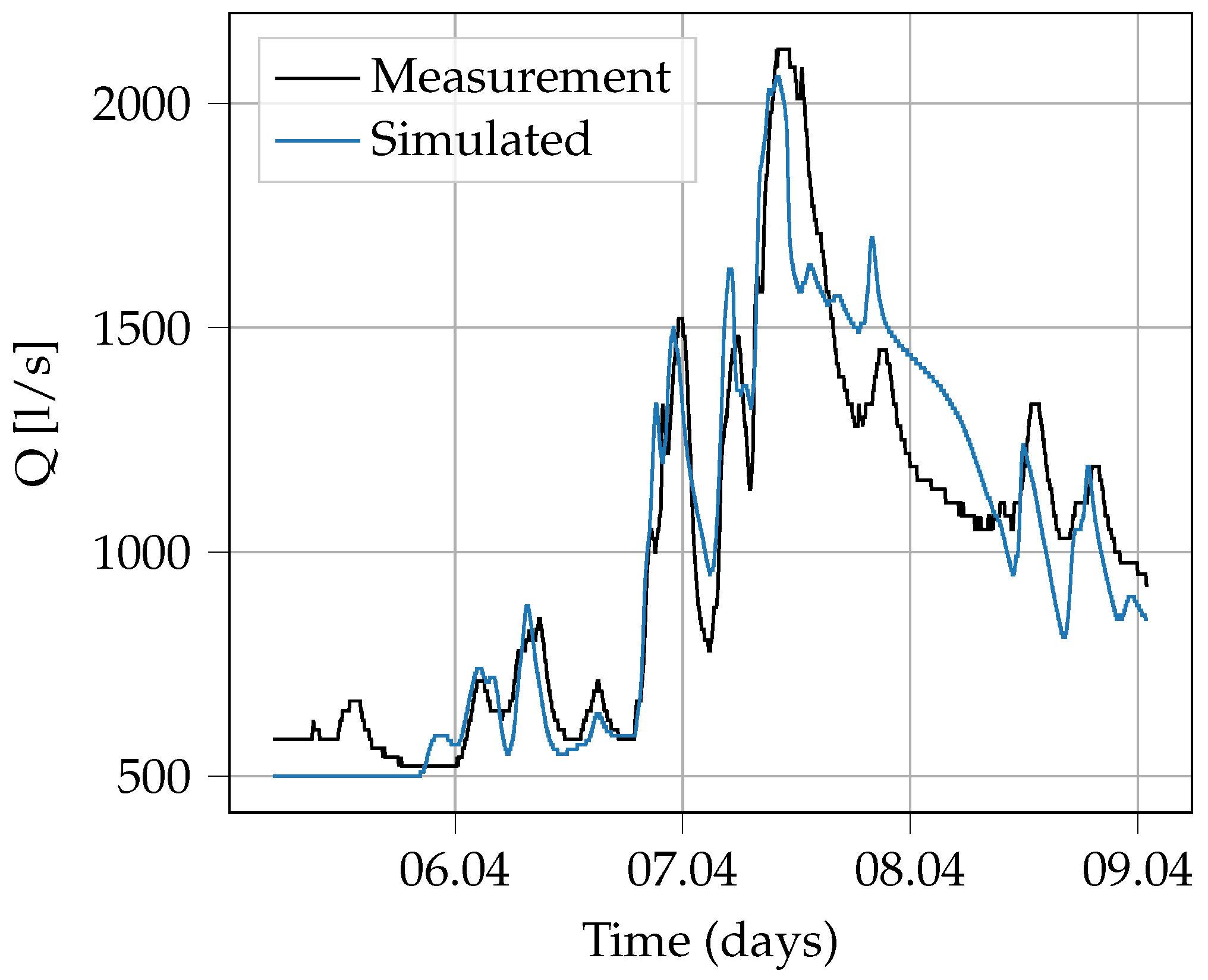
4.2. Results of System Monitoring

For the system monitoring, seven water level sensors, located at the red circles in Figure 3, were used to estimate the state components of the channel network, summarized in Table 1.Note that not all considered sensors were already installed in the real setup.For this study, the data assimilation was validated in the simulation, which means that the presented tool was used to create a simulated truth based on the created 1D1D model (with a 30 cm depression threshold). This was compared to the estimated states of the channel system in the data assimilation process. Therefore, a sample size of 10 min and a number of 15 ensembles was selected for the state estimation scheme. Again, an academic moderate rain event, which is shown in Figure A1, was used to evaluate the convergence behavior of the state estimation. It represents a long-lasting moderate rainfall event, which is applied spatially equivalently. Additionally, a sensor noise with covariance $R=(1\times {10}^{-4})I_7$ with the identity matrix $I_7$ was used for all sensors, while the process noise was applied category-wise using the parameters from

Table A1. Covariances for the considered process noise, depending on the type of modelling element.

Component Type	Depth	(In-)Flow	Runoff
Storages	$1\times {10}^{-2}$	$1\times {10}^{-9}$
Nodes	$1\times {10}^{-2}$	$1\times {10}^{-3}$
Links	$1\times {10}^{-2}$	$1\times {10}^{-4}$
Subcatchments			$1\times {10}^{-15}$

.

Figure 9 displays the mean absolute error (MAE) between the estimated states and the simulated truth of the four component types. Additionally, the evolution of the true water level compared to the minimal, maximal and mean water levels of the corresponding estimated state of the internal model is shown for sensor A in Figure 10.

Since the initial condition of the model is assumed to be unknown, a uniformly distributed initial guess is used, as described in Section 3.2. This results in a high initial deviation, which can be seen in both Figure 9 and Figure 10. However, that deviation is reduced almost every time step at the beginning of the data assimilation process before the mean error stays approximately constant within a range of a couple centimeters or dm${}^3$/s around 1.5 h. Shortly after the rain event starts, the mean absolute error slightly rises but can be reduced again, even before the rain event ends at 10:50. A similar behavior can be observed when looking at the tracking behavior of the water level measured by sensor A, where the estimated state approaches the real state and follows its trajectory, even during the rain event.

Figure 10. Measured water level (black) and minimal (green), mean (blue), maximal (red) estimated water levels at sensor location A.

Figure 10. Measured water level (black) and minimal (green), mean (blue), maximal (red) estimated water levels at sensor location A.

Regarding real-time applicability, it can be said that only a fraction of the sample size has been used for ensemble prediction, whereas further results will follow in Section 4.3. Further investigation showed that the data assimilation using only the measurement information that was available in the real system performed more weakly, which can be traced back to the deteriorated observability properties. This again emphasizes the use of such a digital tool in order to be able to simulatively test and evaluate whether an additional sensor and the planned location can improve the accuracy of the estimated states.

Since the MAE shows the category-wise deviation of the estimated states, the tracking behavior of the unmeasured states is included in this plot. By adjusting the sensor noise or the injected process noise, this behavior can be changed.

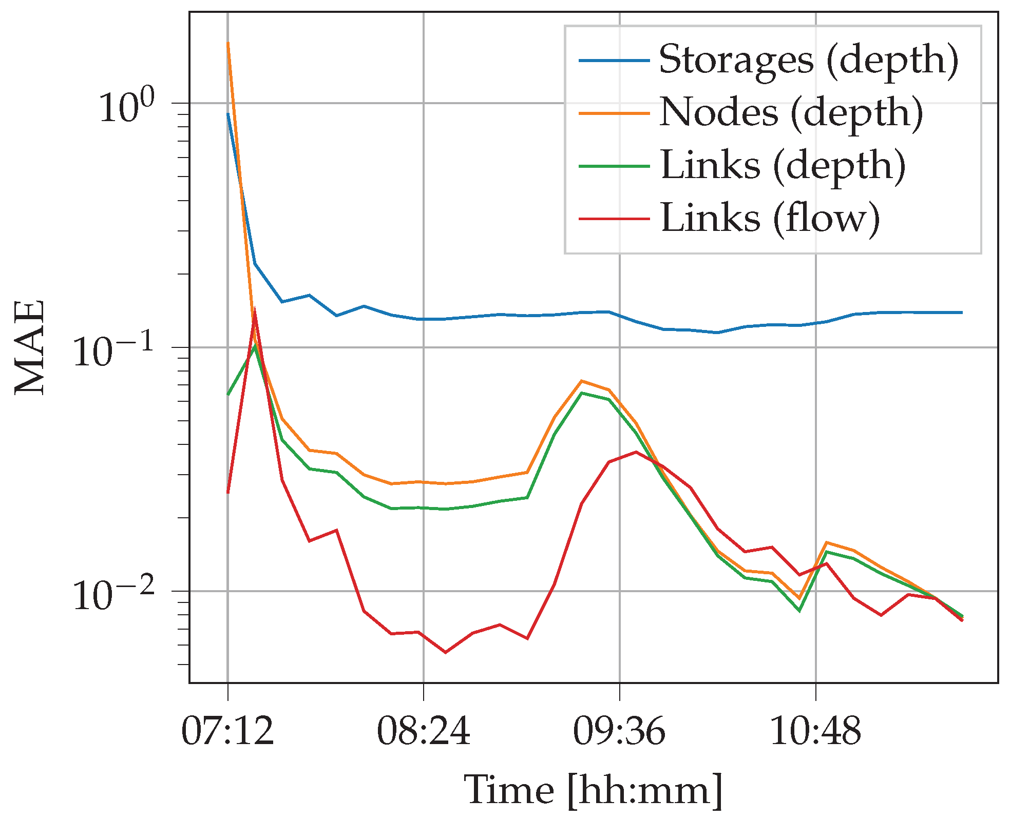
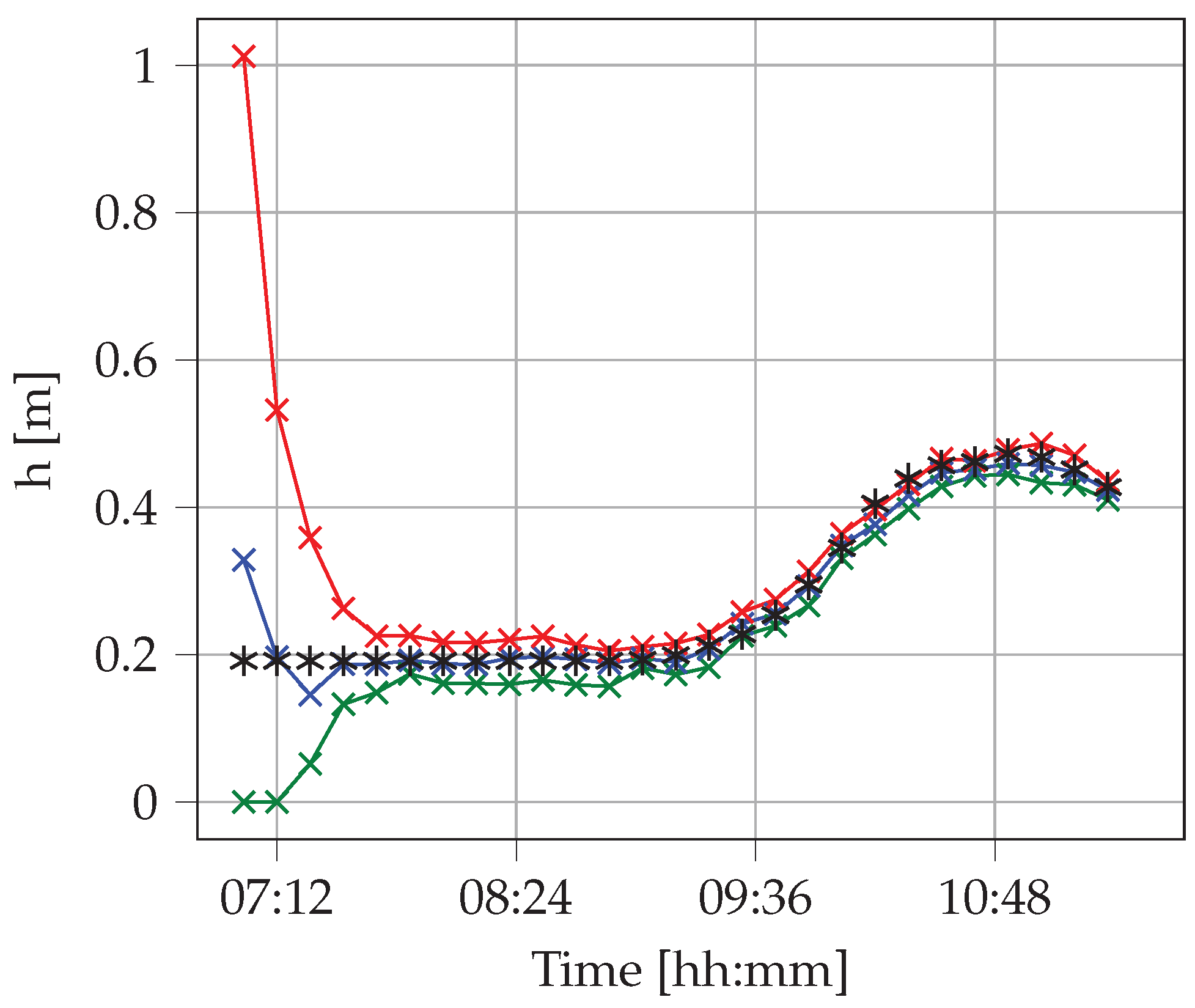
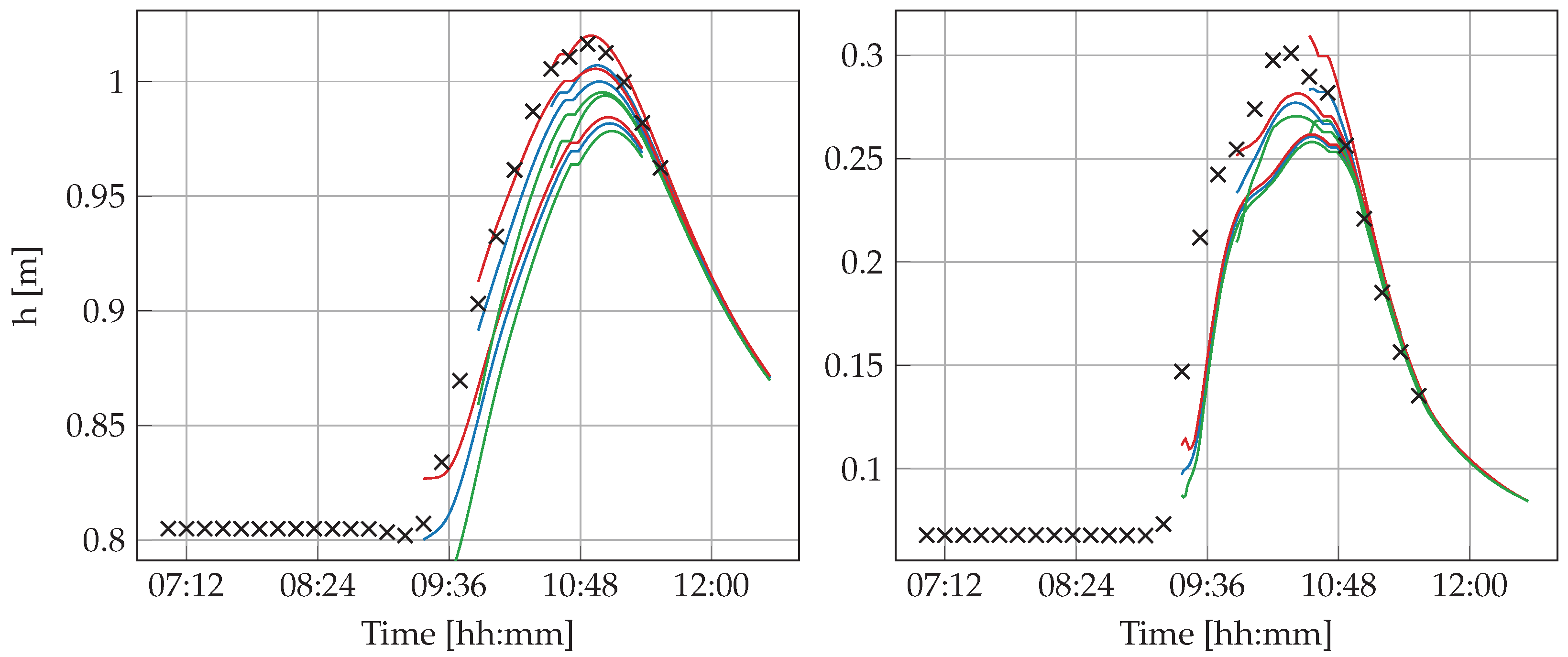
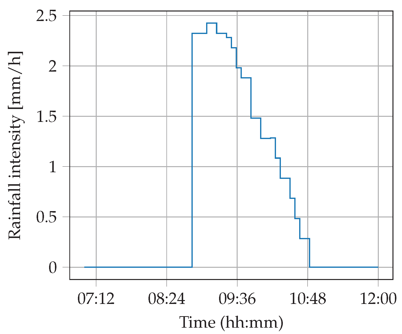
4.3. Results of the Early Warning System

In addition to the estimation of the current state, the potential impact of future scenarios can be predicted based on the dynamic model. To evaluate the prediction quality, again, the channel network was used as the internal model, and the hyper-parameters from Section 4.2 are selected. Additionally, the prediction horizon was chosen to be 2 h, since this is a typical time frame when radar data are used for rainfall prediction. However, for the simulative evaluation, the academic rain scenario displayed in Figure A1 is used, which is assumed to be known a priori.

An extraction of the results for the location of sensors B and C is shown in Figure 11. For clarity, only three predictions and the corresponding trajectory confidence intervals are plotted, whereas data assimilation was performed every 10 min. It can be seen that the first prediction takes the increasing water level caused by the upcoming rain into account but underestimates its impact. As time evolves and additional measurement information is available, the predictions are more aligned with future measurements. Thus, the third prediction that is displayed captures the current and the upcoming water levels accurately while the water level is decreasing after the rain event.

In general, the deviation in the prediction can have different sources. On the one hand, a deviating initial condition will have an impact on the prediction, and on the other hand, model inaccuracies or statistic rain events can yield prediction errors. In reality, predictions should become less accurate with increasing time; thus, the error band should grow with the predicted time. This can be obtained by using an ensemble forecast for the rain or by setting an error band independent from the ensemble trajectories.

Figure 11. Water level prediction at the locations of Sensor B (left) and Sensor C (right) at three time instances compared with the measurements from Sensors B and C, respectively. The measurements are marked in black, while the minimal (green), mean (blue) and maximal (red) water level are obtained from the model predictions.

Figure 11. Water level prediction at the locations of Sensor B (left) and Sensor C (right) at three time instances compared with the measurements from Sensors B and C, respectively. The measurements are marked in black, while the minimal (green), mean (blue) and maximal (red) water level are obtained from the model predictions.

With respect to the hyper-parameters, such as the ensemble size and the forecast prediction horizon, real-time ability can be achieved for sampling intervals of 10 and even for 5 min.

5. Conclusions

An efficient approach for 1D1D urban stormwater modelling is recalled, and the underlying data processing for the automatic creation of digital models, e.g., in the open-source software SWMM, is presented. All system information is stored in a database, whereafter the channel and surface model are created based on two threshold conditions to adapt to the level of detail. Furthermore, an ensemble Kalman filter-based data assimilation approach has been applied using the open-source tool that is introduced in this work. Both the modelling and the state estimation are carried out for the stormwater system of the case area in Flensburg city.

Comparing the efficient 1D1D model with the real measurement shows satisfying results, which indicates sufficient model accuracy. Both the peak flow as well as the rain-dependent rural runoff are captured. For further testing and evaluation, more and especially more intense rainfall events are required. This will result in faster runoff, especially in the urban areas. Regarding the computational effort and the level of detail with respect to the depression threshold, 30 cm appears to be sufficient for this use case. However, if a more detailed model is required, the automatic scheme enables a fast method to refine the spatial resolution. Furthermore, the authors recommend using data assimilation to obtain the estimated state, including information about all elements of the internal model. It has been shown that the estimated states approach the real measurements after a small warm-up phase of approximately 1 h when the initial states were not known a priori. Due to observability restrictions, the internal model has been chosen to cover the channel system. The observability of the system should be further analyzed, and the automatic creation of the SWMM models can be optimized with respect to the observability of the internal model, such that even surface elements could be taken into account.

The main goal for future work is now to connect the monitoring and early warning systems to the real plant such that it can act as a digital twin. In this way, the system helps operators to know where overflows can be expected in the upcoming hours. As shown in the literature, approaches based on machine learning are also able to model a rain network quickly and rather accurately after sufficient training [10]. An idea to combine these approaches is the possibility to use HiFi models for short-term simulations to identify the current state, while neuronal networks are used for early warning under the consideration of several different rain scenarios. However, it should be considered that all data-based techniques need a wide range of training data to capture the dynamics for a wide range of scenarios. Since a digital twin additionally aims to support the process decision-making, a real-time control scheme can be developed based on the actual state estimate, which is obtained from the data assimilation scheme. Finally, to further reduce the computational time to be able to simulate more scenarios, GPU parallelization could be used.

References

1. IPCC. Climate Change 2022: Mitigation of Climate Change. Contribution of Working Group III to the Sixth Assessment Report of the Intergovernmental Panel on Climate Change; Cambridge University Press: Cambridge, MA, USA; Cambridge, UK, 2022. [Google Scholar] [CrossRef]
2. Skougaard Kaspersen, P.; Høegh Ravn, N.; Arnbjerg-Nielsen, K.; Madsen, H.; Drews, M. Comparison of the impacts of urban development and climate change on exposing European cities to pluvial flooding. Hydrol. Earth Syst. Sci. 2017, 21, 4131–4147. [Google Scholar] [CrossRef] [Green Version]
3. Botín-Sanabria, D.M.; Mihaita, A.S.; Peimbert-García, R.E.; Ramírez-Moreno, M.A.; Ramírez-Mendoza, R.A.; Lozoya-Santos, J.d.J. Digital Twin Technology Challenges and Applications: A Comprehensive Review. Remote Sens. 2022, 14, 1335. [Google Scholar] [CrossRef]
4. Liu, M.; Fang, S.; Dong, H.; Xu, C. Review of digital twin about concepts, technologies, and industrial applications. J. Manuf. Syst. 2021, 58, 346–361. [Google Scholar] [CrossRef]
5. Fuller, A.; Fan, Z.; Day, C.; Barlow, C. Digital Twin: Enabling Technologies, Challenges and Open Research. IEEE Access 2020, 8, 108952–108971. [Google Scholar] [CrossRef]
6. Pedersen, A.N.; Borup, M.; Brink-Kjær, A.; Christiansen, L.E.; Mikkelsen, P.S. Living and Prototyping Digital Twins for Urban Water Systems: Towards Multi-Purpose Value Creation Using Models and Sensors. Water 2021, 13, 592. [Google Scholar] [CrossRef]
7. Bartos, M.; Kerkez, B. Pipedream: An interactive digital twin model for natural and urban drainage systems. Environ. Model. Softw. 2021, 144, 105120. [Google Scholar] [CrossRef]
8. Thorndahl, S.; Poulsen, T.S.; Bøvith, T.; Borup, M.; Ahm, M.; Nielsen, J.E.; Grum, M.; Rasmussen, M.R.; Gill, R.; Mikkelsen, P.S. Comparison of short-term rainfall forecasts for model-based flow prediction in urban drainage systems. Water Sci. Technol. 2013, 68, 472–478. [Google Scholar] [CrossRef]
9. Petrucci, G.; Bonhomme, C. The dilemma of spatial representation for urban hydrology semi-distributed modelling: Trade-offs among complexity, calibration and geographical data. J. Hydrol. 2014, 517, 997–1007. [Google Scholar] [CrossRef]
10. Palmitessa, R.; Grum, M.; Engsig-Karup, A.P.; Löwe, R. Accelerating hydrodynamic simulations of urban drainage systems with physics-guided machine learning. Water Res. 2022, 223, 118972. [Google Scholar] [CrossRef]
11. Guo, K.; Guan, M.; Yu, D. Urban surface water flood modelling—A comprehensive review of current models and future challenges. Hydrol. Earth Syst. Sci. 2021, 25, 2843–2860. [Google Scholar] [CrossRef]
12. Nkwunonwo, U.; Whitworth, M.; Baily, B. A review of the current status of flood modelling for urban flood risk management in the developing countries. Sci. Afr. 2020, 7, e00269. [Google Scholar] [CrossRef]
13. Mannina, G. (Ed.) New Trends in Urban Drainage Modelling; Springer Cham: Cham, Switzerland, 2018. [Google Scholar] [CrossRef]
14. Bach, P.M.; Rauch, W.; Mikkelsen, P.S.; McCarthy, D.T.; Deletic, A. A critical review of integrated urban water modelling—Urban drainage and beyond. Environ. Model. Softw. 2014, 54, 88–107. [Google Scholar] [CrossRef]
15. Maksimović, Č.; Prodanović, D.; Boonya-Aroonnet, S.; Leitao, J.P.; Djordjević, S.; Allitt, R. Overland flow and pathway analysis for modelling of urban pluvial flooding. J. Hydraul. Res. 2009, 47, 512–523. [Google Scholar] [CrossRef]
16. Dong, B.; Xia, J.; Zhou, M.; Li, Q.; Ahmadian, R.; Falconer, R.A. Integrated modeling of 2D urban surface and 1D sewer hydrodynamic processes and flood risk assessment of people and vehicles. Sci. Total Environ. 2022, 827, 154098. [Google Scholar] [CrossRef]
17. Leandro, J.; Chen, A.S.; Djordjević, S.; Savić, D.A. Comparison of 1D/1D and 1D/2D Coupled (Sewer/Surface) Hydraulic Models for Urban Flood Simulation. J. Hydraul. Eng. 2009, 135, 495–504. [Google Scholar] [CrossRef]
18. Jensen, L.; Paludan, B.; Nielsen, N.; Edinger, K. Large scale 1D-1D surface modelling tool for urban water planning. In Proceedings of the Novatech 2010—7ème Conférence internationale sur les techniques et stratégies durables pour la gestion des eaux urbaines par temps de pluie/7th International Conference on Sustainable Techniques and Strategies for Urban Water Management; Brelot, E., Ed.; GRAIE: Lyon, France, 2010; Congrès trisannuel Novatech; pp. 1–10. [Google Scholar]
19. Zhao, G.; Mark, O.; Balstrøm, T.; Jensen, M.B. A Sink Screening Approach for 1D Surface Network Simplification in Urban Flood Modelling. Water 2022, 14, 963. [Google Scholar] [CrossRef]
20. Pina, R.D.; Ochoa-Rodriguez, S.; Simões, N.E.; Mijic, A.; Marques, A.S.; Maksimović, V. Semi- vs. Fully-Distributed Urban Stormwater Models: Model Set Up and Comparison with Two Real Case Studies. Water 2016, 8, 58. [Google Scholar] [CrossRef] [Green Version]
21. Zhao, G.; Balstrøm, T.; Mark, O.; Jensen, M. Multi-Scale Target-Specified Sub-Model Approach for Fast Large-Scale High-Resolution 2D Urban Flood Modelling. Water 2021, 13, 259. [Google Scholar] [CrossRef]
22. Leitão, J.P.; Simães, N.E.; Maksimović, V.; Ferreira, F.; Prodanović, D.; Matos, J.S.; Sá Marques, A. Real-time forecasting urban drainage models: Full or simplified networks? Water Sci. Technol. 2010, 62, 2106–2114. [Google Scholar] [CrossRef]
23. Djordjević, S.; Prodanović, D.; Maksimović, V. An approach to simulation of dual drainage. Water Sci. Technol. 1999, 39, 95–103. [Google Scholar] [CrossRef]
24. Mark, O.; Weesakul, S.; Apirumanekul, C.; Aroonnet, S.B.; Djordjević, S. Potential and limitations of 1D modelling of urban flooding. J. Hydrol. 2004, 299, 284–299. [Google Scholar] [CrossRef]
25. Ferrans, P.; Torres, M.N.; Temprano, J.; Rodríguez Sánchez, J.P. Sustainable Urban Drainage System (SUDS) modeling supporting decision-making: A systematic quantitative review. Sci. Total Environ. 2022, 806, 150447. [Google Scholar] [CrossRef] [PubMed]
26. Rossman, L. Storm Water Management Model. Available online: https://www.epa.gov/water-research/storm-water-management-model-swmm (accessed on 22 September 2022).
27. DHI. MIKE URBAN Product Page. Available online: https://www.mikepoweredbydhi.com/products (accessed on 22 September 2022).
28. Lund, N.S.V.; Madsen, H.; Mazzoleni, M.; Solomatine, D.; Borup, M. Assimilating flow and level data into an urban drainage surrogate model for forecasting flows and overflows. J. Environ. Manag. 2019, 248, 109052. [Google Scholar] [CrossRef]
29. Thrysøe, C.; Arnbjerg-Nielsen, K.; Borup, M. Identifying fit-for-purpose lumped surrogate models for large urban drainage systems using GLUE. J. Hydrol. 2019, 568, 517–533. [Google Scholar] [CrossRef]
30. Baumann, H.; Schaum, A.; Meurer, T. Data-driven control-oriented reduced order modeling for open channel flows. IFAC-PapersOnLine 2022, 55, 193–199. [Google Scholar] [CrossRef]
31. García, L.; Barreiro-Gomez, J.; Escobar, E.; Téllez, D.; Quijano, N.; Ocampo-Martinez, C. Modeling and real-time control of urban drainage systems: A review. Adv. Water Resour. 2015, 85, 120–132. [Google Scholar] [CrossRef] [Green Version]
32. Lund, N.S.V.; Falk, A.K.V.; Borup, M.; Madsen, H.; Mikkelsen, P.S. Model predictive control of urban drainage systems: A review and perspective towards smart real-time water management. Crit. Rev. Environ. Sci. Technol. 2018, 48, 279–339. [Google Scholar] [CrossRef]
33. Litrico, X.; Fromion, V. Modeling and Control of Hydrosystems; Springer: London, UK, 2009. [Google Scholar]
34. Lund, N.S.V.; Borup, M.; Madsen, H.; Mark, O.; Mikkelsen, P.S. CSO Reduction by Integrated Model Predictive Control of Stormwater Inflows: A Simulated Proof of Concept Using Linear Surrogate Models. Water Resour. Res. 2020, 56, e2019WR026272. [Google Scholar] [CrossRef]
35. Svensen, J.L.; Sun, C.; Cembrano, G.; Puig, V. Chance-constrained stochastic MPC of Astlingen urban drainage benchmark network. Control Eng. Pract. 2021, 115, 104900. [Google Scholar] [CrossRef]
36. Kalman, R.E. A new approach to linear filtering and prediction problems. Trans. ASME–J. Basic Eng. 1960, 82, 35–45. [Google Scholar] [CrossRef] [Green Version]
37. Sakov, P.; Oke, P.R. A deterministic formulation of the ensemble Kalman filter: An alternative to ensemble square root filters. Tellus A 2008, 60, 361–371. [Google Scholar] [CrossRef] [Green Version]
38. Borup, M.; Grum, M.; Madsen, H.; Mikkelsen, P.S. A partial ensemble Kalman filtering approach to enable use of range limited observations. Stoch. Environ. Res. Risk Assess. 2015, 29, 119–129. [Google Scholar] [CrossRef] [Green Version]
39. Hansen, L.S.; Borup, M.; Møller, A.; Mikkelsen, P.S. Flow Forecasting using Deterministic Updating of Water Levels in Distributed Hydrodynamic Urban Drainage Models. Water 2014, 6, 2195–2211. [Google Scholar] [CrossRef] [Green Version]
40. Das, J.; Manikanta, V.; Teja, K.N.; Umamahesh, N.V. Two decades of ensemble flood forecasting: A state-of-the-art on past developments, present applications and future opportunities. Hydrol. Sci. J. 2022, 67, 477–493. [Google Scholar] [CrossRef]
41. Palmitessa, R.; Mikkelsen, P.; Law, A.; Borup, M. Data assimilation in hydrodynamic models for system-wide soft sensing and sensor validation for urban drainage tunnels. J. Hydroinform. 2020, 23. [Google Scholar] [CrossRef]
42. de Saint-Venant, A.B. Théorie du mouvement non permanent des eaux, avec application aux crues des rivières et a l’introduction de marées dans leurs lits. C. R. L’Académie Des Sci. 1871, 73, 147–154, 237–240. [Google Scholar]
43. Pedersen, A.N.; Brink-Kjær, A.; Mikkelsen, P.S. All models are wrong, but are they useful? Assessing reliability across multiple sites to build trust in urban drainage modelling. EGUsphere 2022, 2022, 1–32. [Google Scholar] [CrossRef]
44. Evensen, G. Data Assimilation: The Ensemble Kalman Filter, 2nd ed.; Springer: Berlin/Heidelberg, Germany, 2009. [Google Scholar]
45. Evensen, G. The Ensemble Kalman Filter: Theoretical formulation and practical implementation. Ocean Dyn. 2003, 53, 343–367. [Google Scholar] [CrossRef]
46. Nijmeier, H.; van der Schaft, A. Nonlinear Dynamical Control Systems; Springer: New York, NY, USA, 1990. [Google Scholar]
47. Liu, Y.; Slotine, J.; Barabasi, A. Observability of complex systems. Proc. Natl. Acad. Sci. USA 2012, 110, 2460–2465. [Google Scholar] [CrossRef]
48. Pichler, M. Swmm_API: API for Reading, Manipulating and Running SWMM-Projects with Python (0.2.0.16); Zenodo: Geneve, Switzerland, 2022. [Google Scholar] [CrossRef]
49. McDonnell, B.; Ratliff, K.; Tryby, M.; Wu, J.; Mullapudi, A. PySWMM: The Python Interface to Stormwater Management Model (SWMM). J. Open Source Softw. 2020, 5, 2292. [Google Scholar] [CrossRef]
50. Burger, G.; Sitzenfrei, R.; Kleidorfer, M.; Rauch, W. Parallel flow routing in SWMM 5. Environ. Model. Softw. 2014, 53, 27–34. [Google Scholar] [CrossRef]
Figure 1. Schematic representation of the 1D1D overland flow modelling.
Modelling 03 00030 g001
Figure 2. Schematic overview of data processing for efficient 1D1D modelling.
Modelling 03 00030 g002
Figure 3. Overview of the stormwater network of Flensburg modelled with a pipe diameter threshold of 30 cm. Nodes of the model are highlighted with green dots, while the links are colored in blue. The red circles correspond to the points at which level sensors are considered later for system monitoring.
Modelling 03 00030 g003
Figure 4. Identified subarea center points for extraction of the case area with 10 cm (black dots), 30 cm (magenta squares) and 50 cm (green circles) thresholds, respectively.
Modelling 03 00030 g004
Figure 5. Illustration of the identified subareas for the extraction marked in Figure 4 with a depression threshold of 10 cm. (a) Identified subareas (colored) and corresponding subarea center points (black dots). (b) Overflow interconnections (marked with blue dots) of the identified subareas.
Modelling 03 00030 g005
Figure 6. Schematic overview of data assimilation procedure (left) and the general folder structure of the early warning system tool (right).
Modelling 03 00030 g006
Figure 7. Comparison of measured and calculated flow for a rain event in April 2022.
Modelling 03 00030 g007
Figure 8. Flood maps of a 100-year event with different depression thresholds for the surface modelling. The subarea center points of a 10 cm and 30 cm depression are marked with black dots and mangeta squares, respectively. The surcharge water level reaches from 0 to 1 m (color map white to red).
Modelling 03 00030 g008
Figure 9. Category-wise mean absolute error (MAE) of the estimated states.
Modelling 03 00030 g009