Inelastic Behavior of Steel and Composite Frame Structure Subjected to Earthquake Loading


Abstract
:1. Introduction
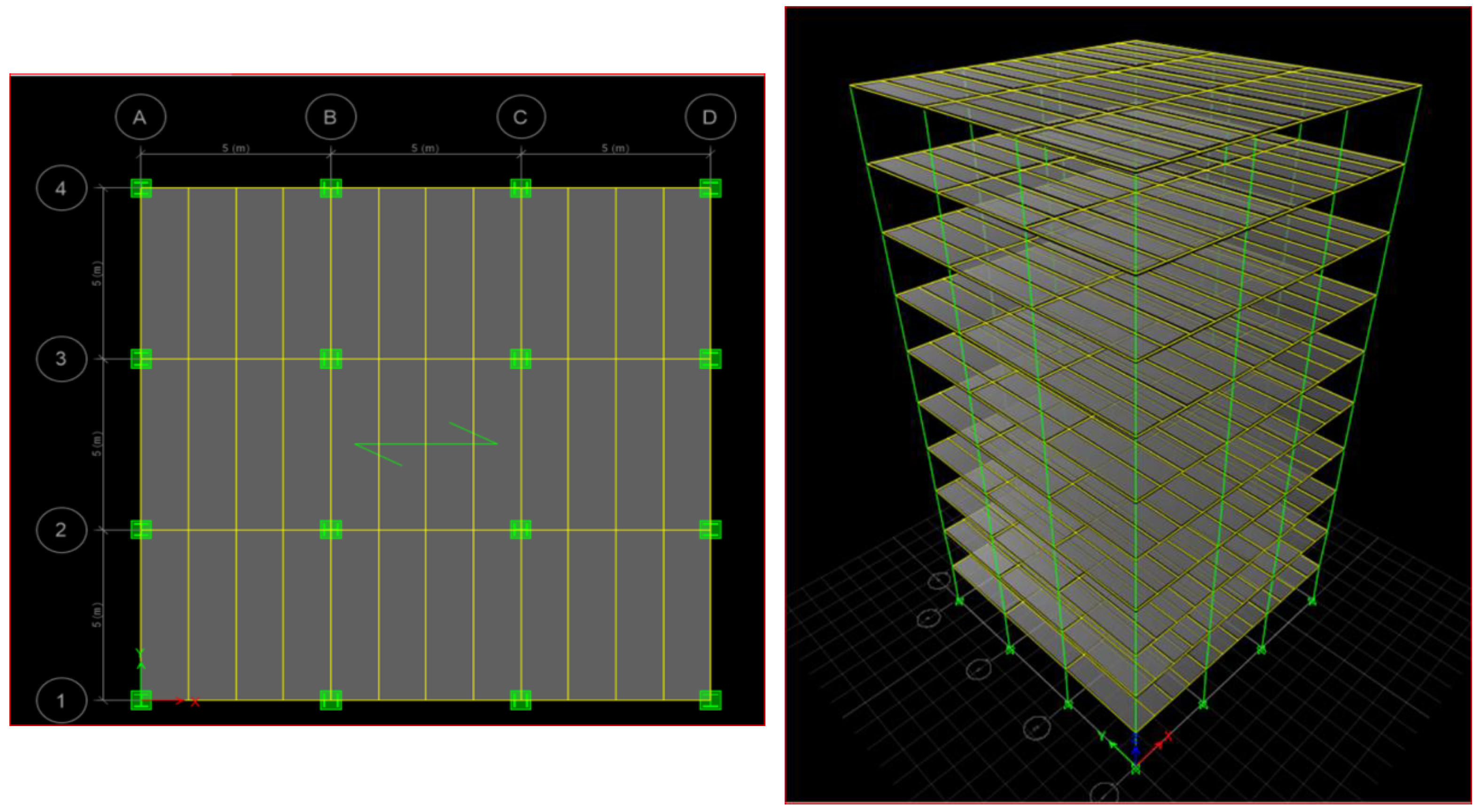
2. Methodology and Structural Description
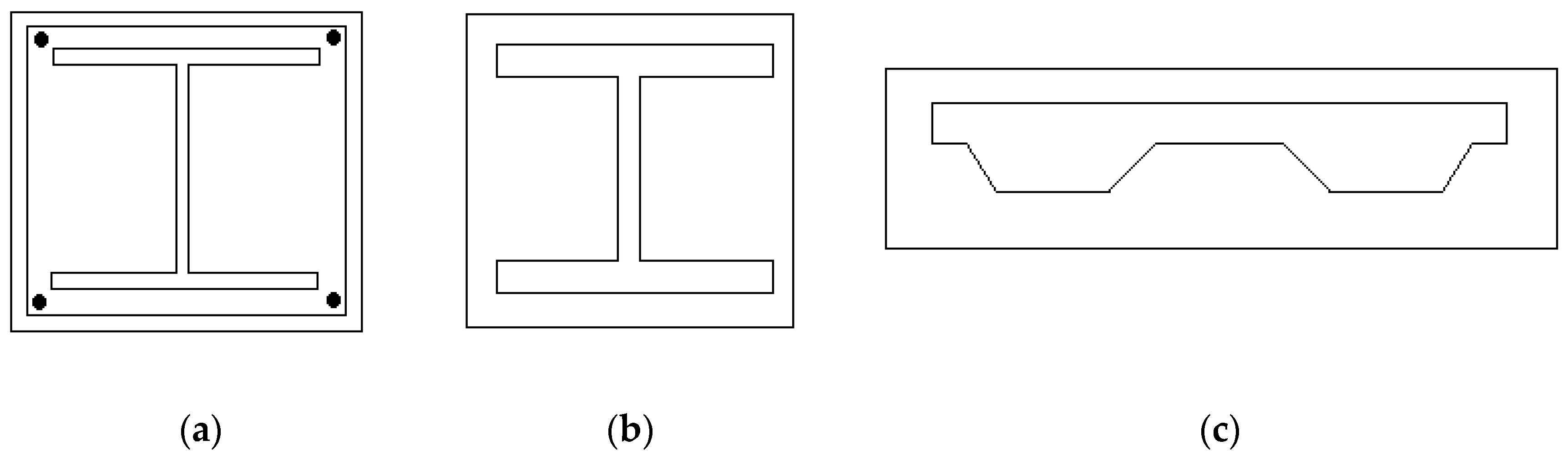
3. Load Details and Design Sections
4. Results and Discussions
4.1. Modal Analysis
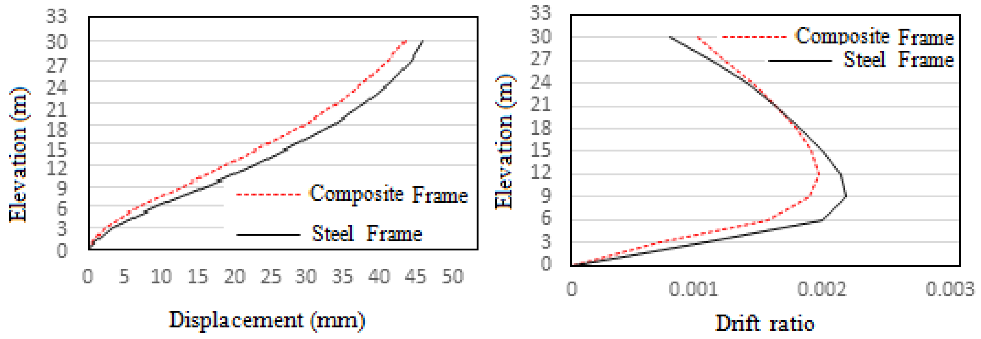
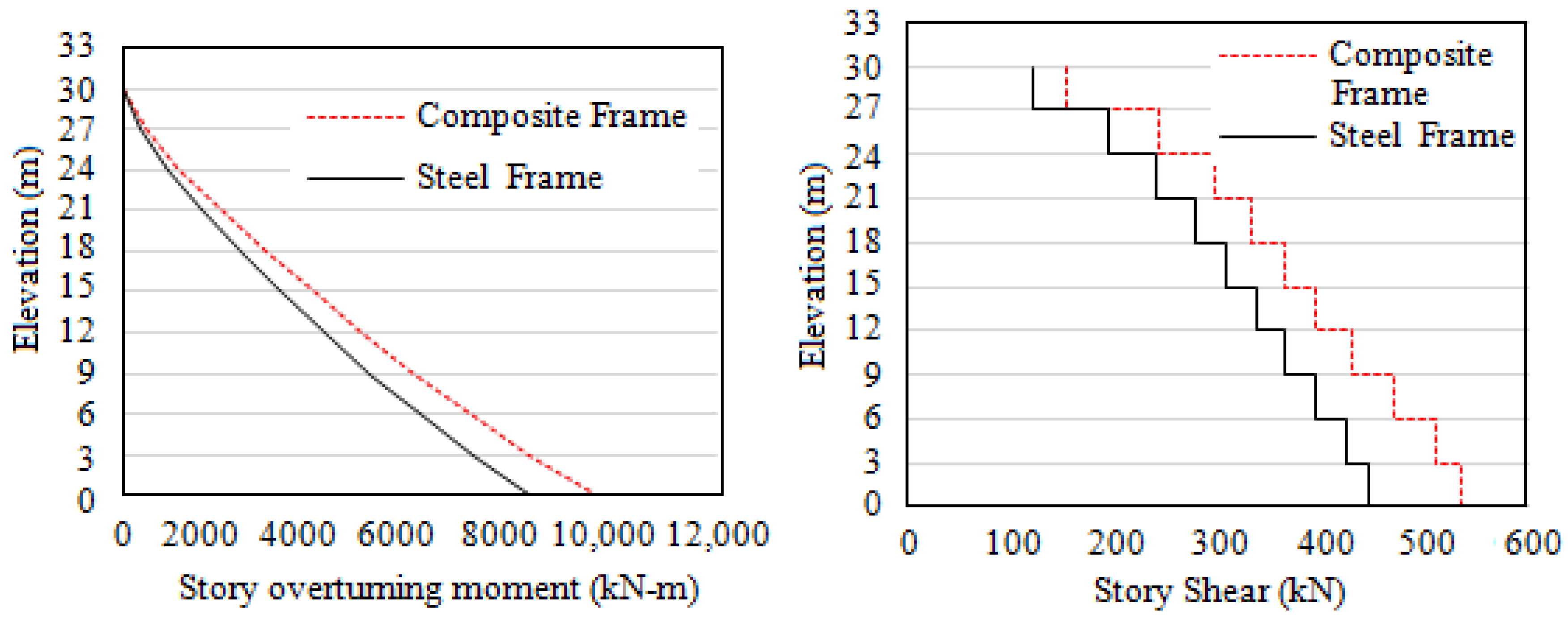
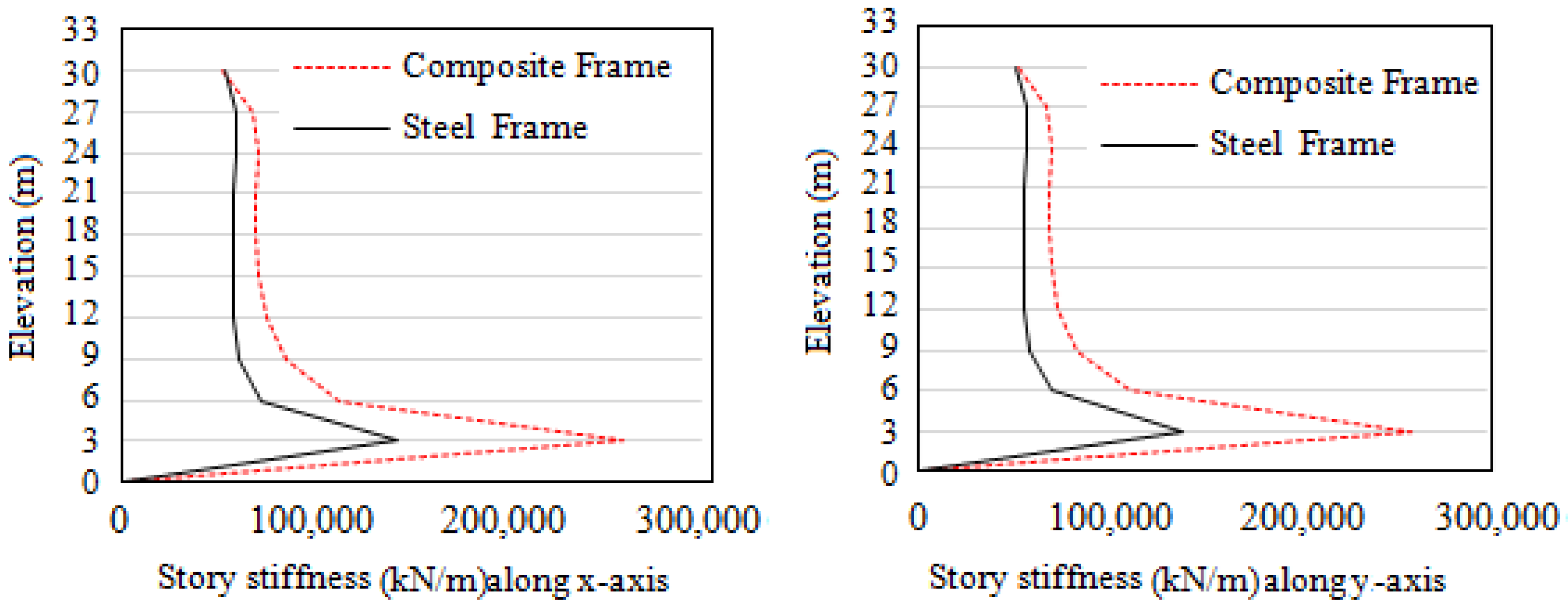
4.2. Response Spectrum Analysis
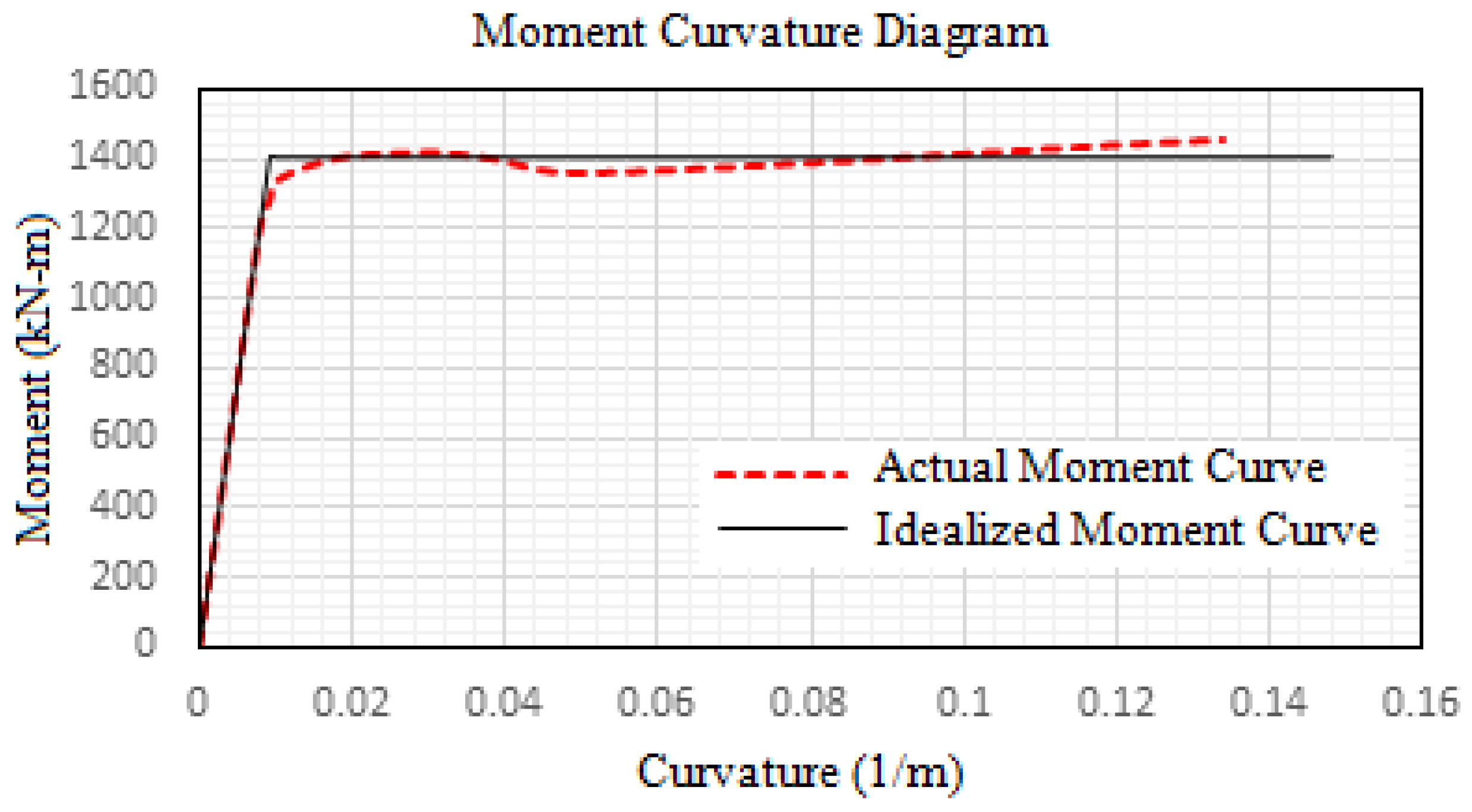
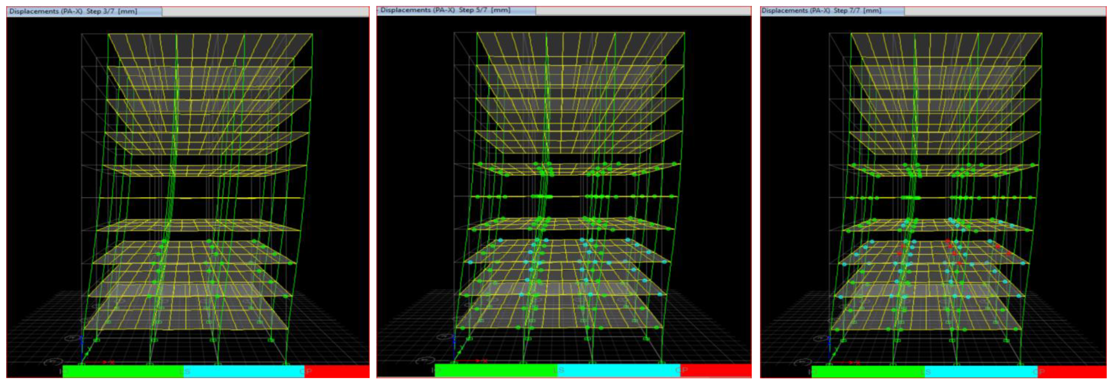
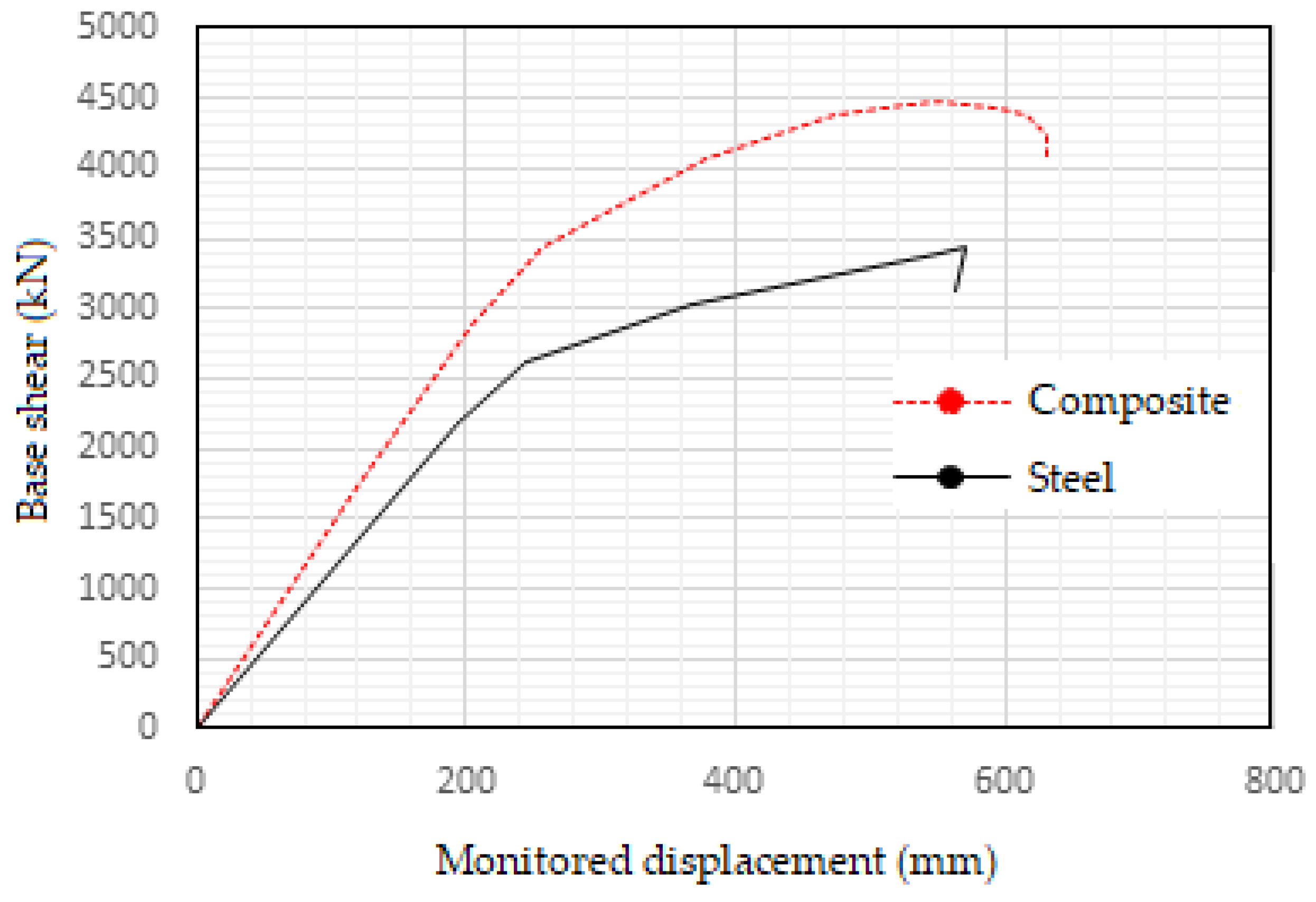
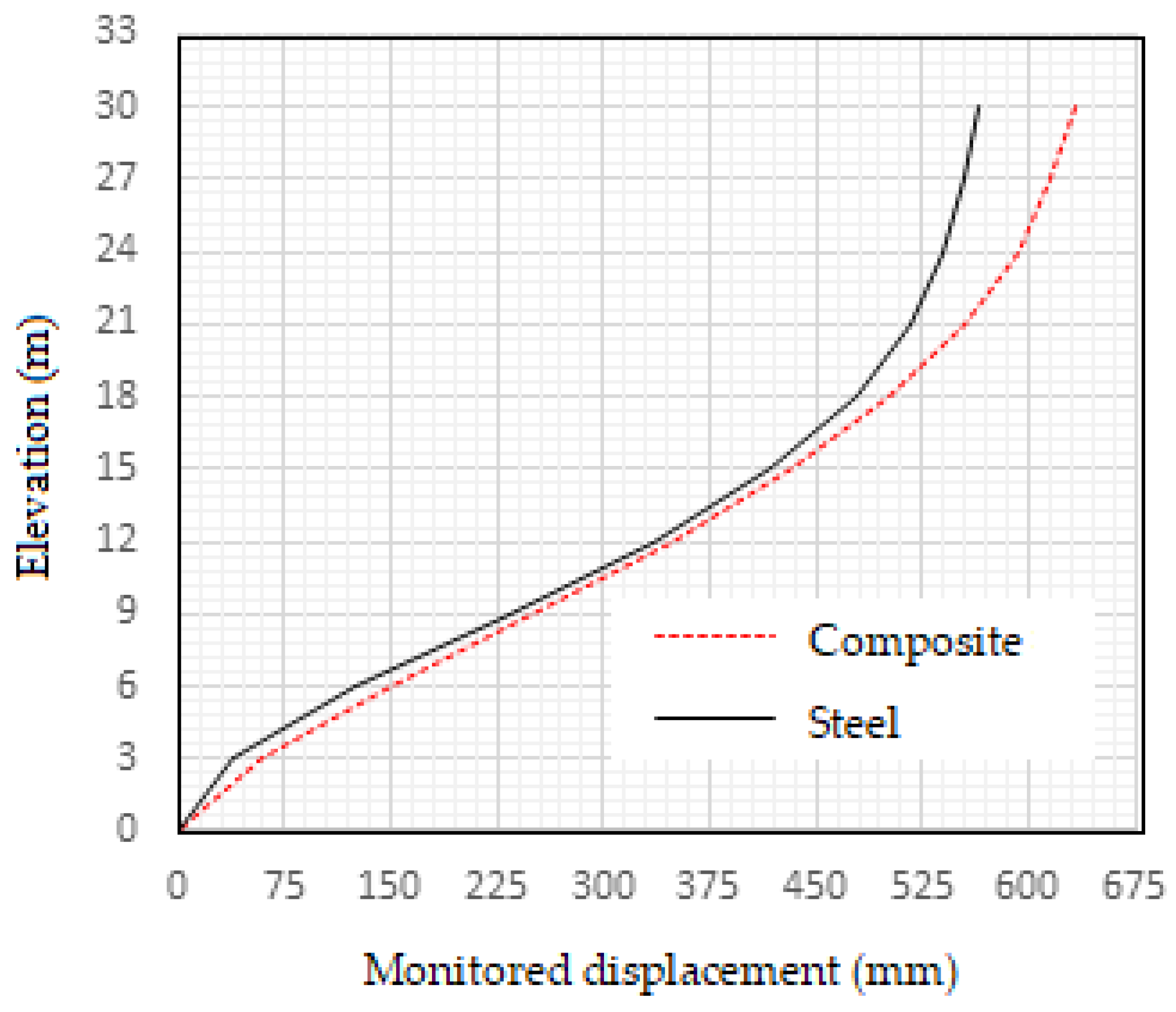
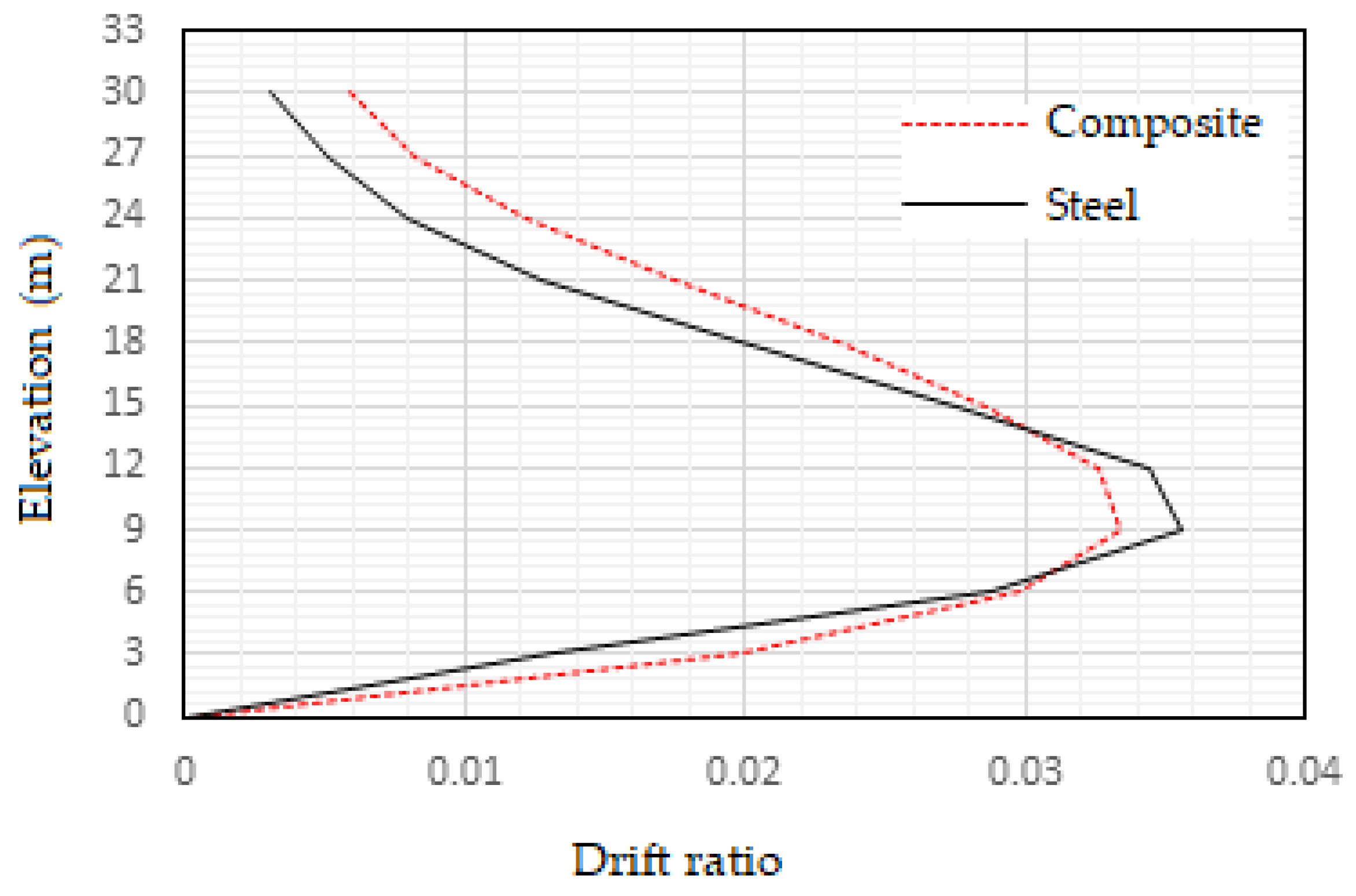
4.3. Pushover Analysis
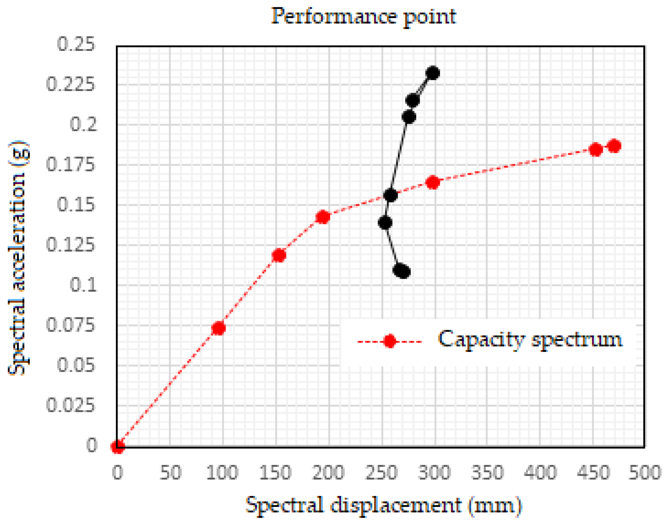
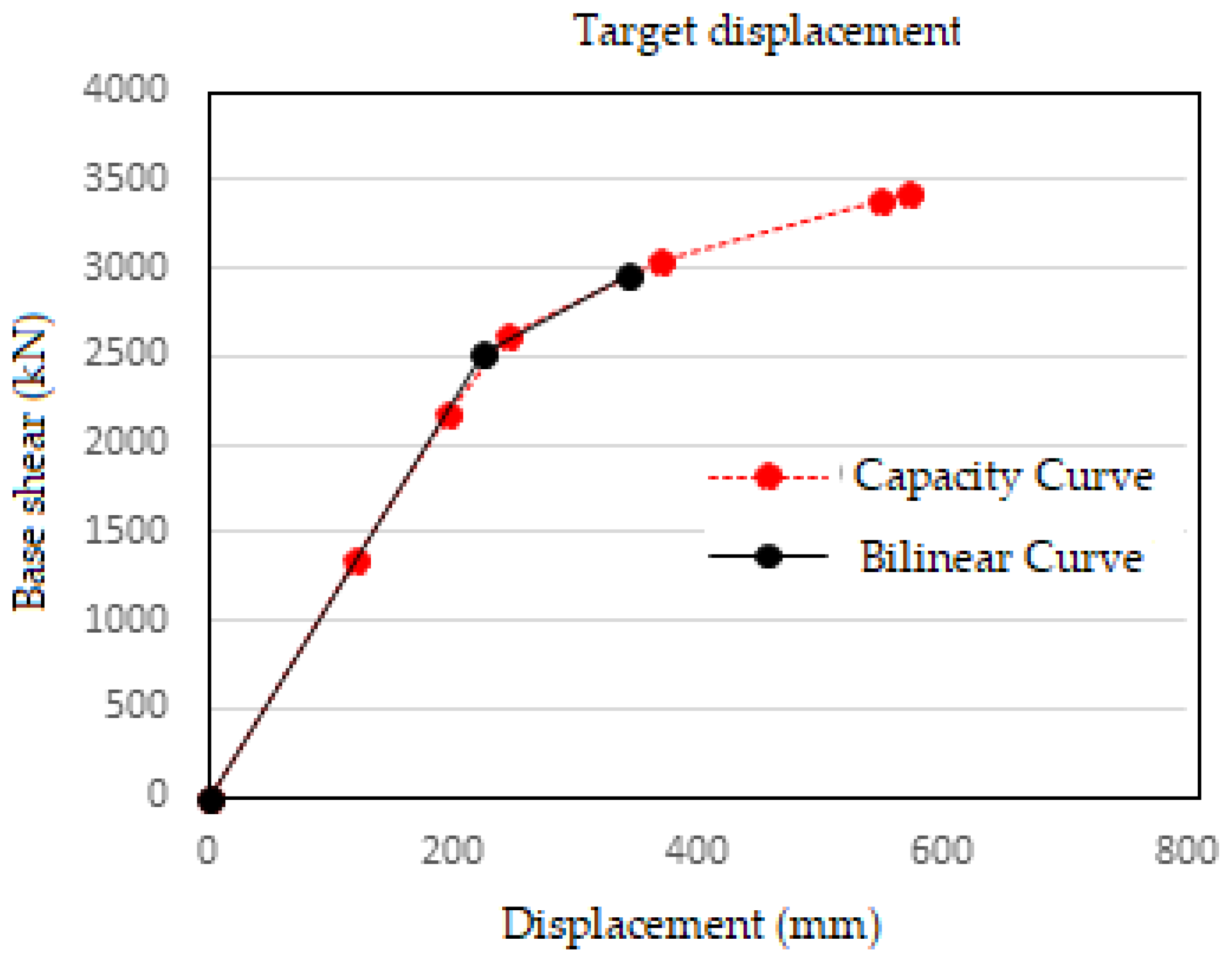
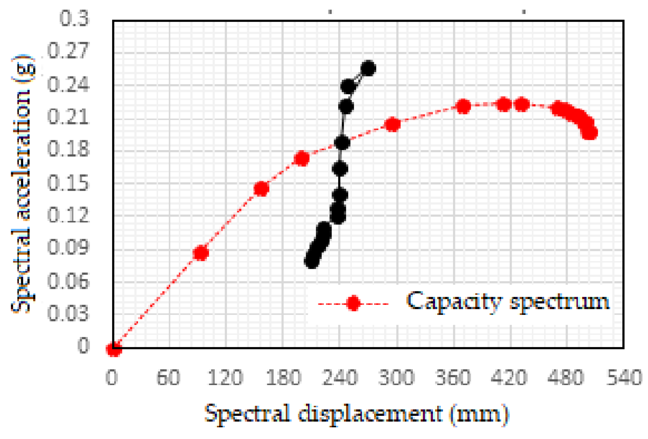
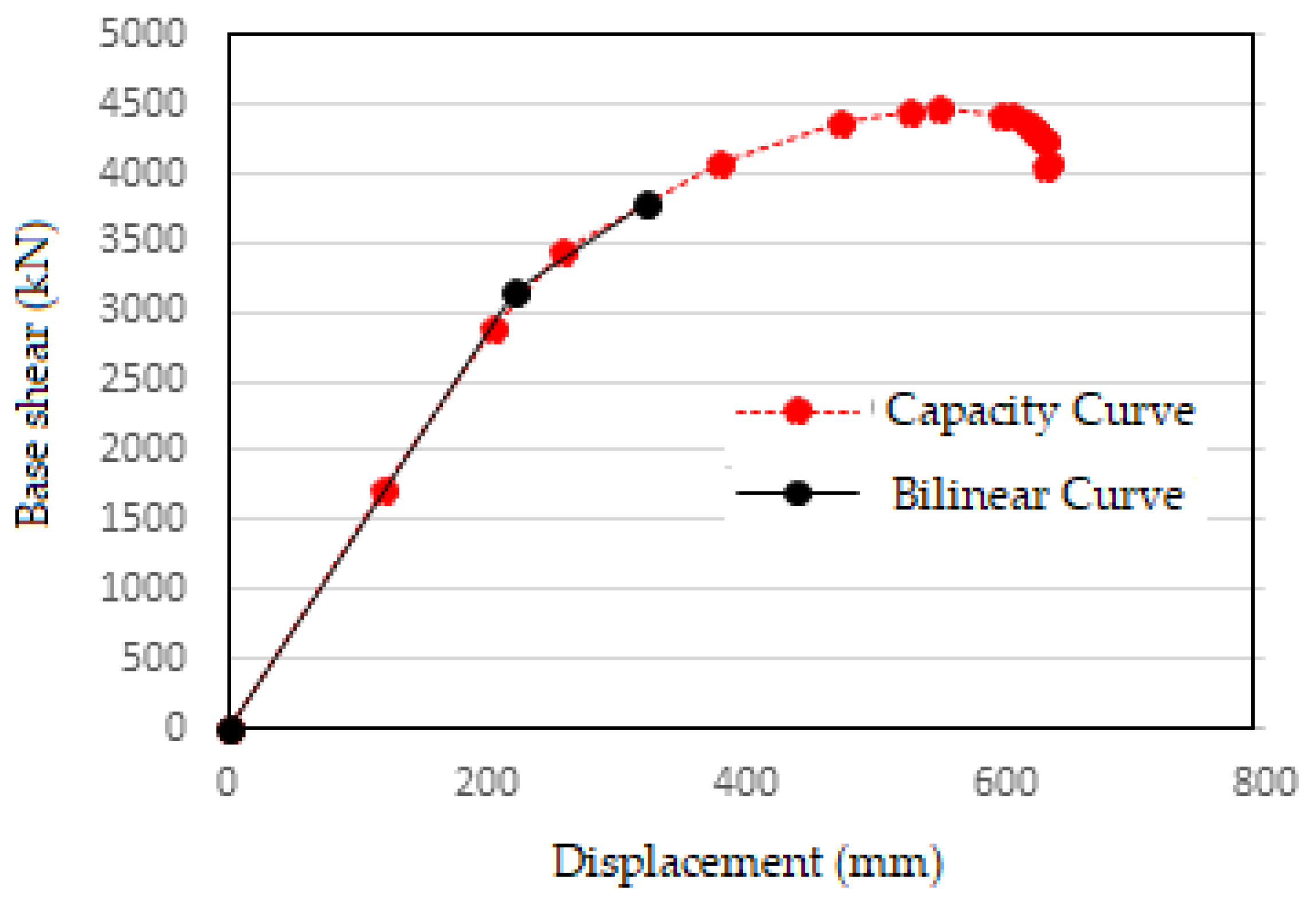
4.4. Comparison of Performance Point and Target Displacement for Frames
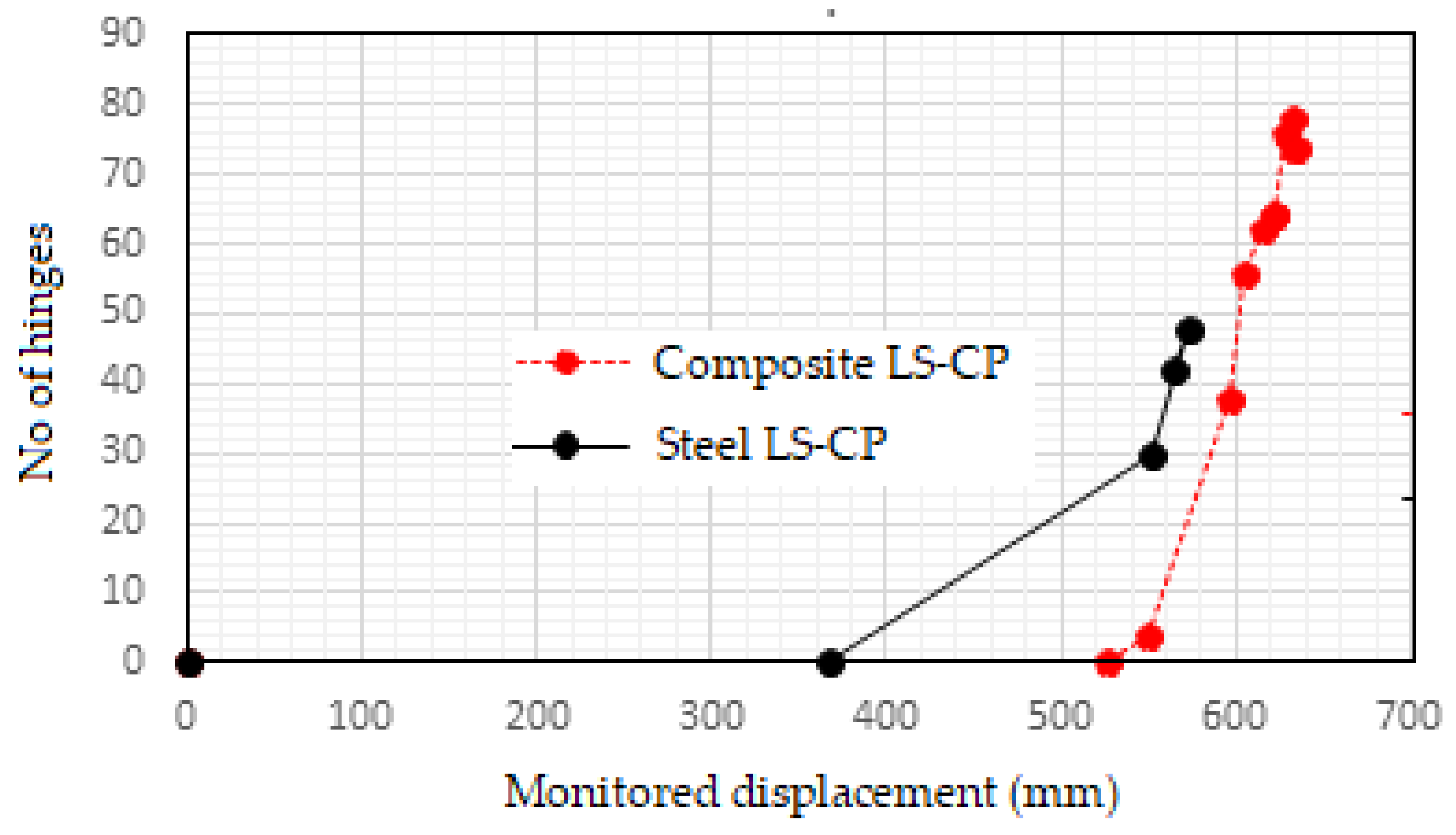
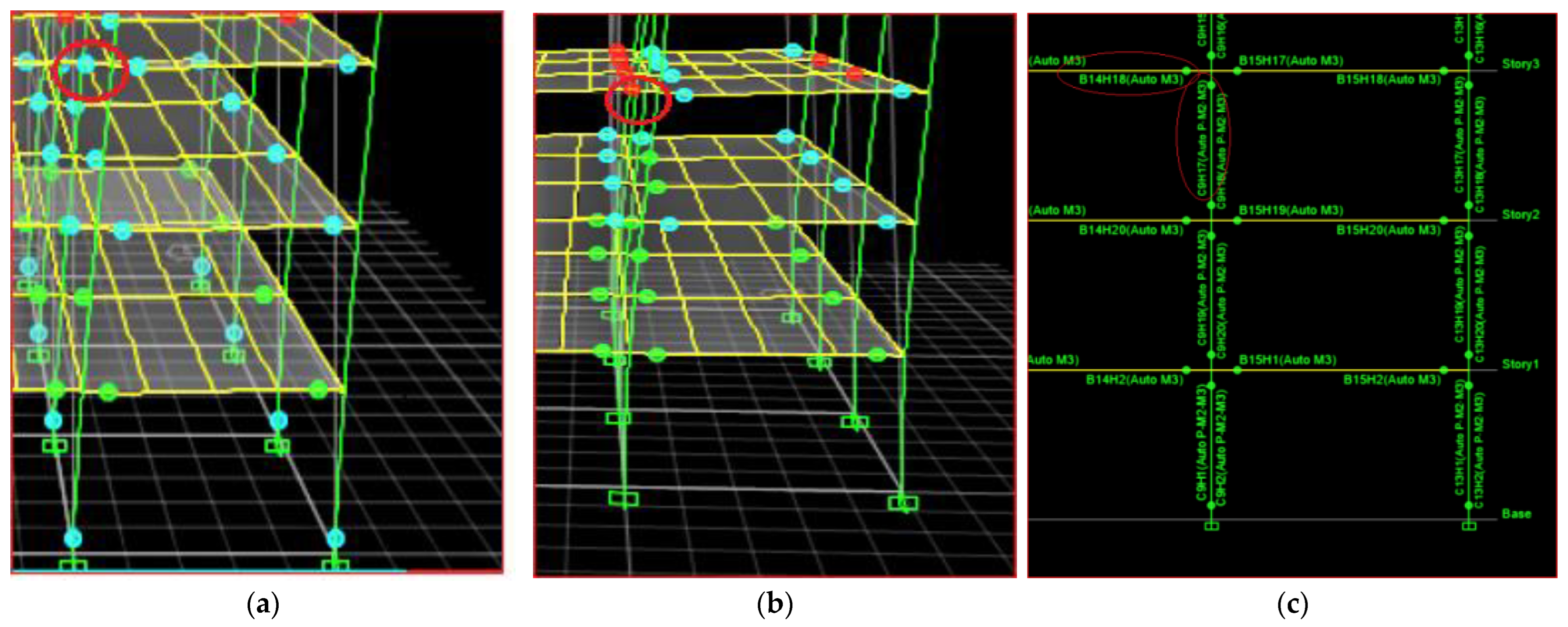
4.5. Comparison of Progressive Hinge Formation in Steel and Composite Frame
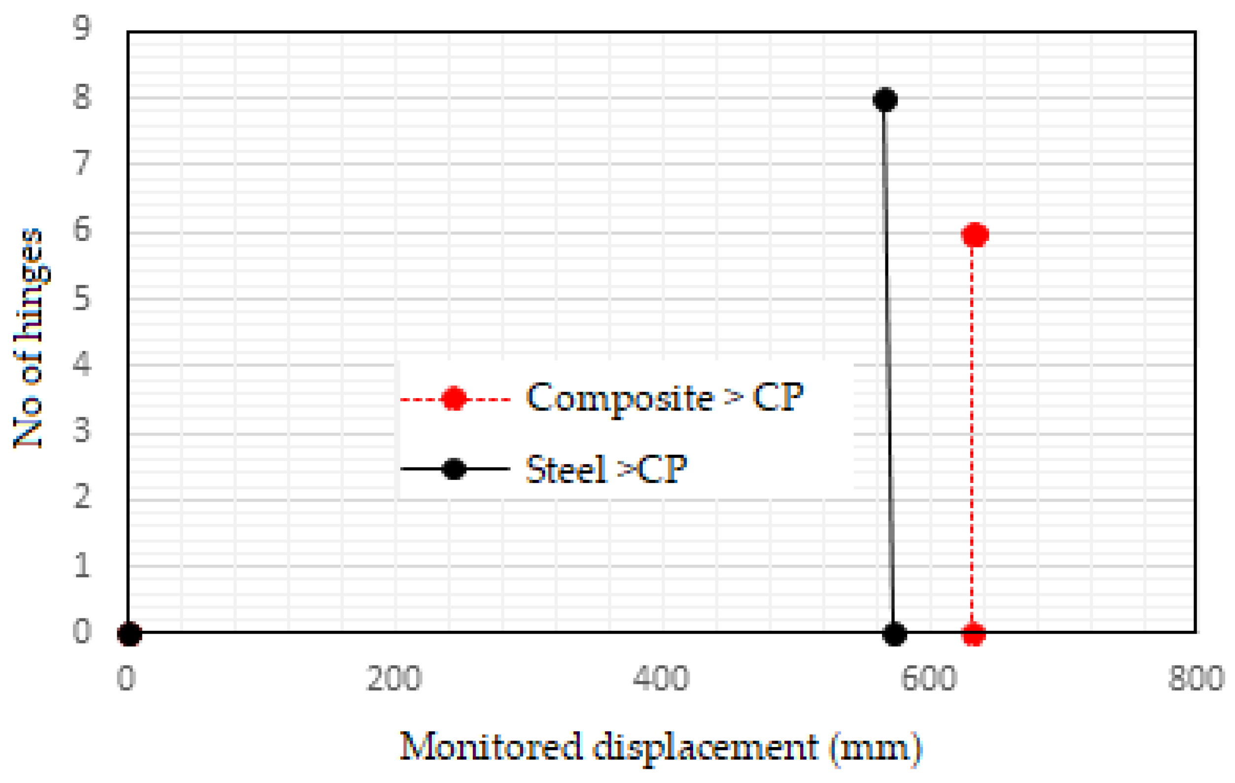
4.6. Number of Hinges Crossing the CP Threshold
- (i)
- Global stiffness of the frames:
- (a)
- Composite frame:
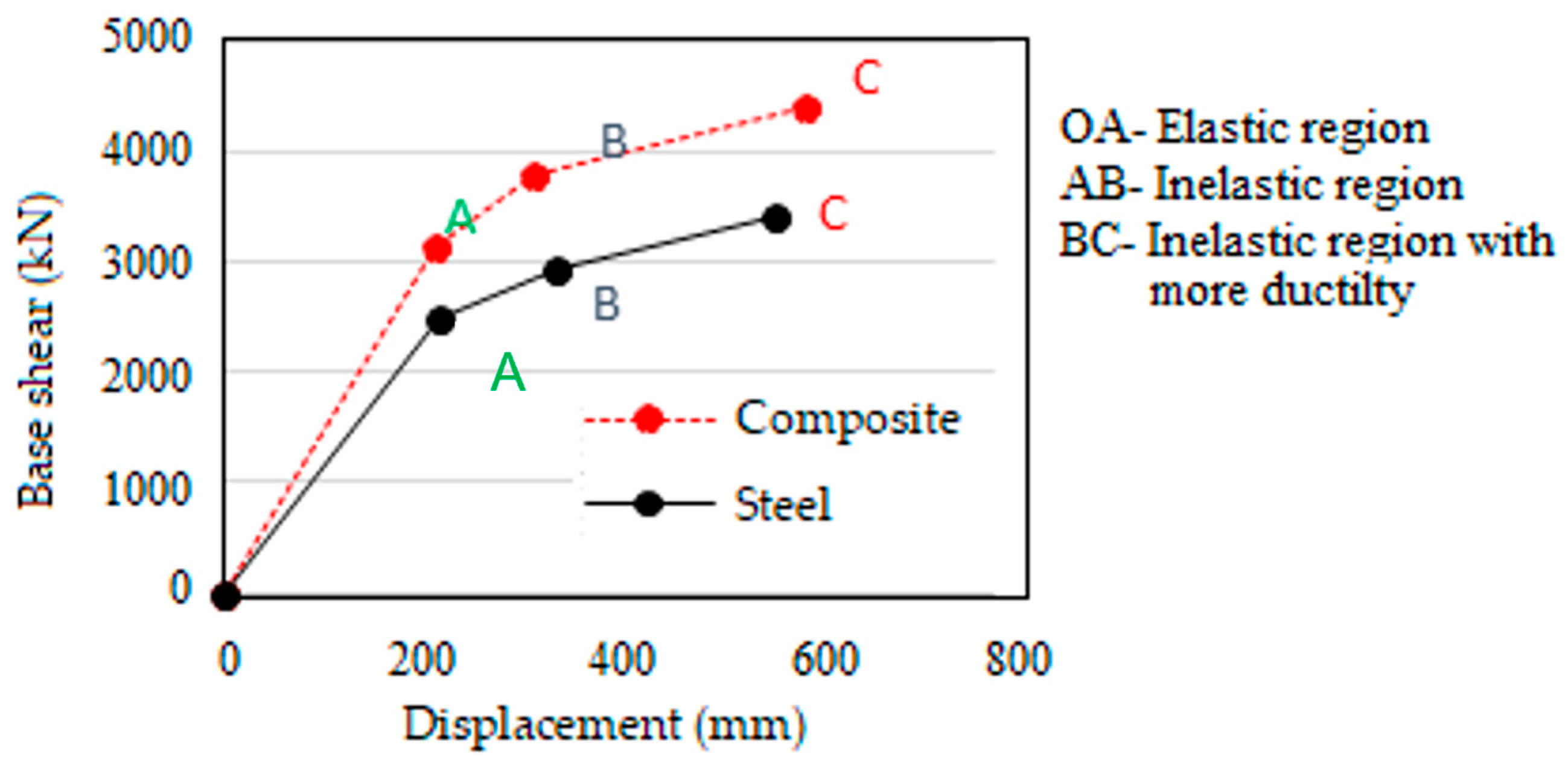
Stiffness in the region AB = (3787.86 − 3140.79)/(322.69 − 220.009) = 6.3 kN/mm = 6301.8 kN/m (Inelastic region)
Stiffness in the region BC = (4414.63 − 3787.86)/(605.24 − 322.69) = 2.22 kN/mm = 2218.2 kN/m (Inelastic region)
- (b)
- Steel frame:
Stiffness in the region AB = (2954.46 − 2508.35)/(344.01 − 223.71) = 3.71 kN/mm = 3708.5 kN/m (Inelastic region)
Stiffness in the region BC = (3432.52 − 2954.46)/(572.01 − 344.01) = 2.09 kN/mm = 2096.7 kN/m (Inelastic region)
- (ii)
- Ductility:
- (a)
- Composite frame:
- (b)
- Steel frame:
- (iii)
- Lateral strength:
- (a)
- Composite frame:
- (b)
- Steel frame:
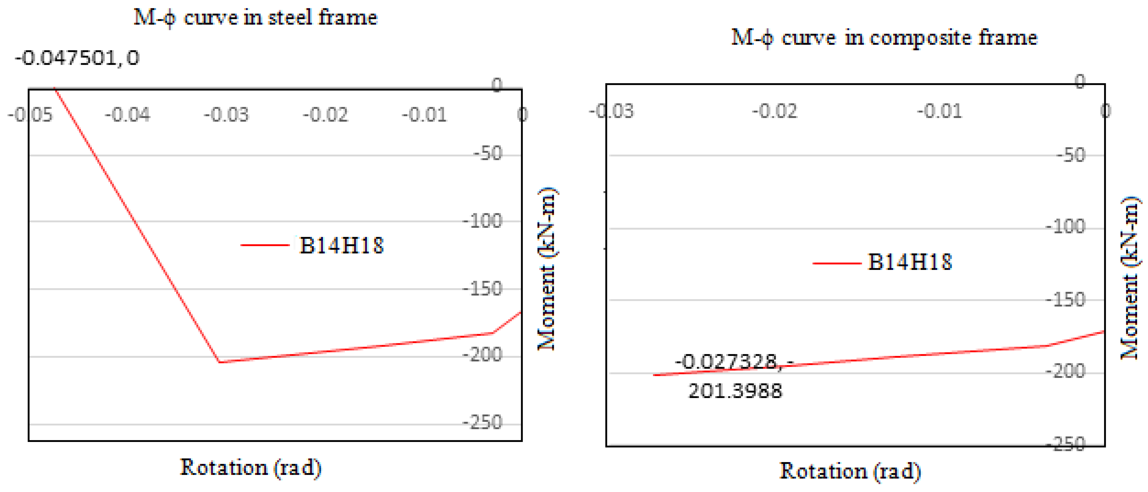
4.7. Moment Rotation Curves
B14H18 and C9H17 Comparison
4.8. Time History Analysis
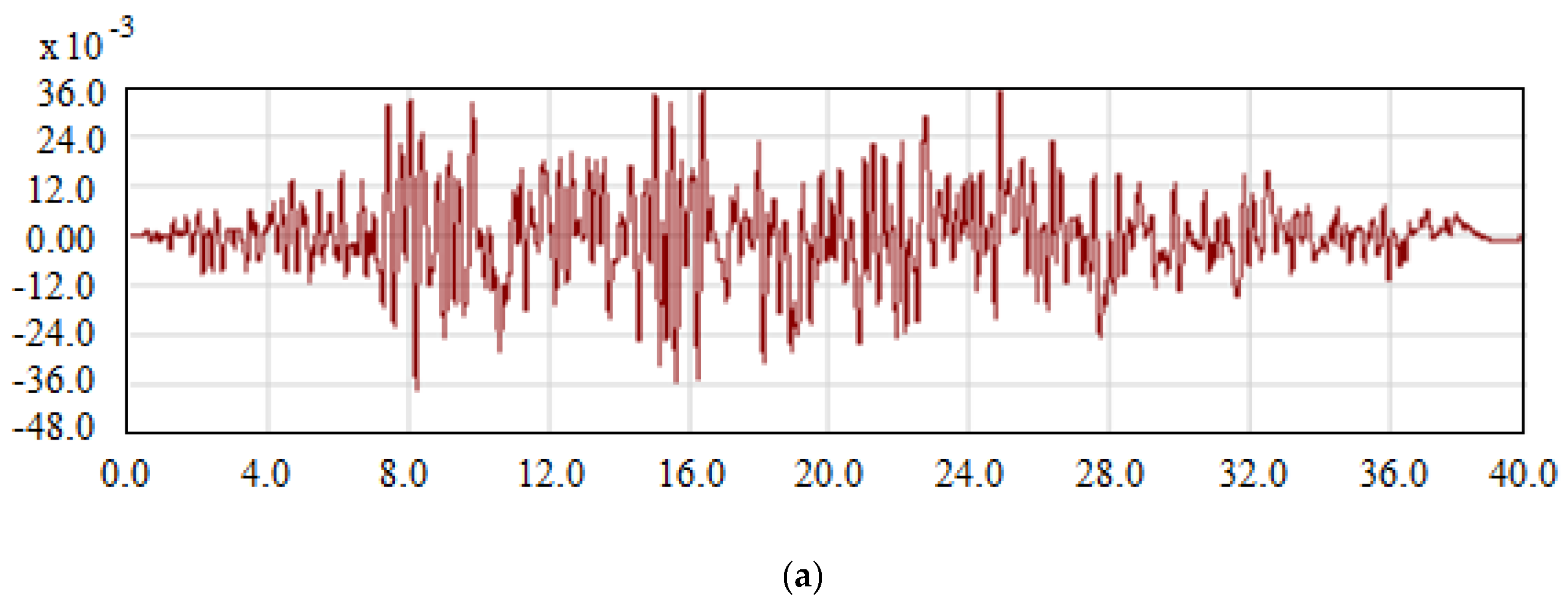
4.9. Earthquake Details
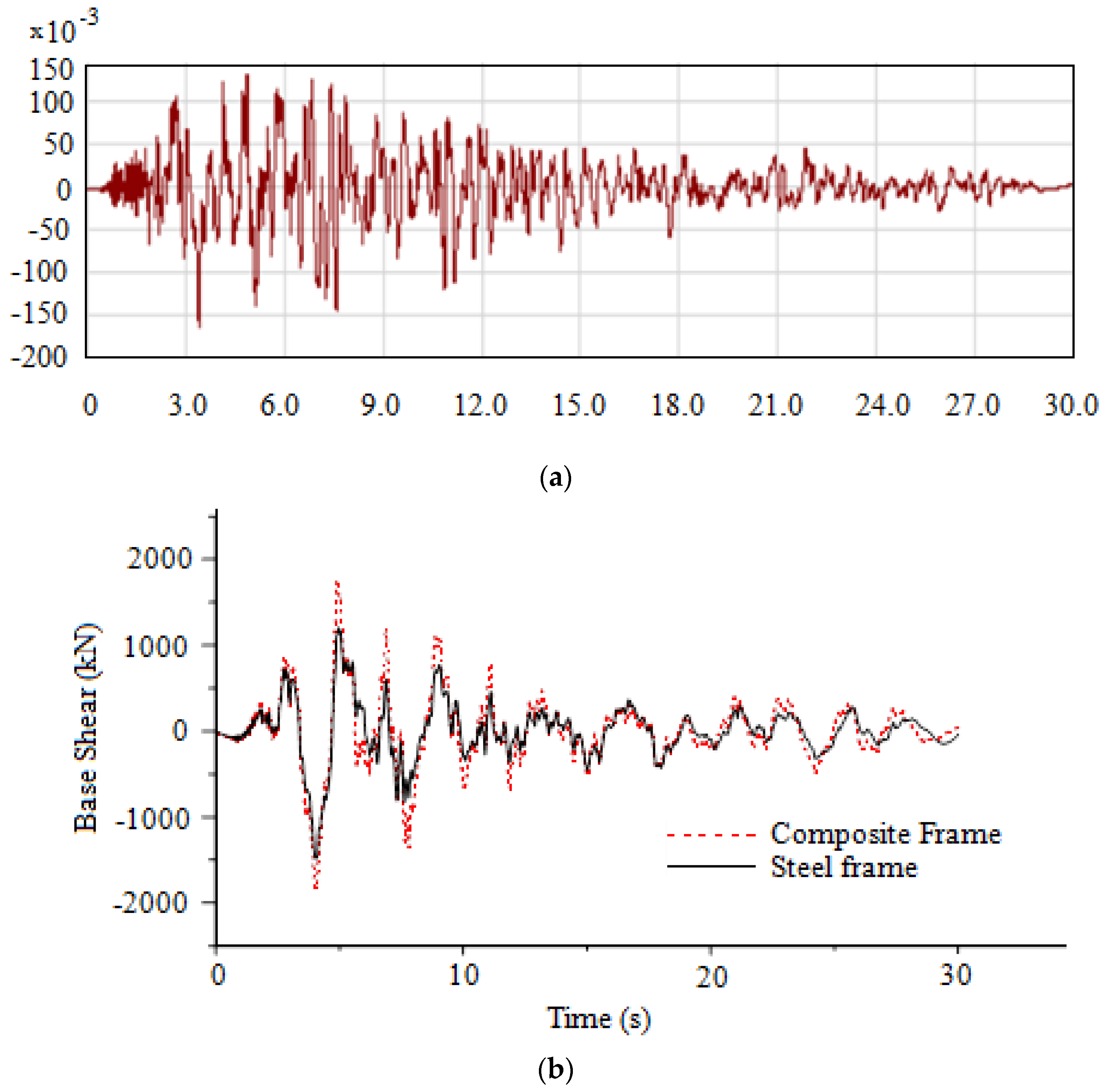
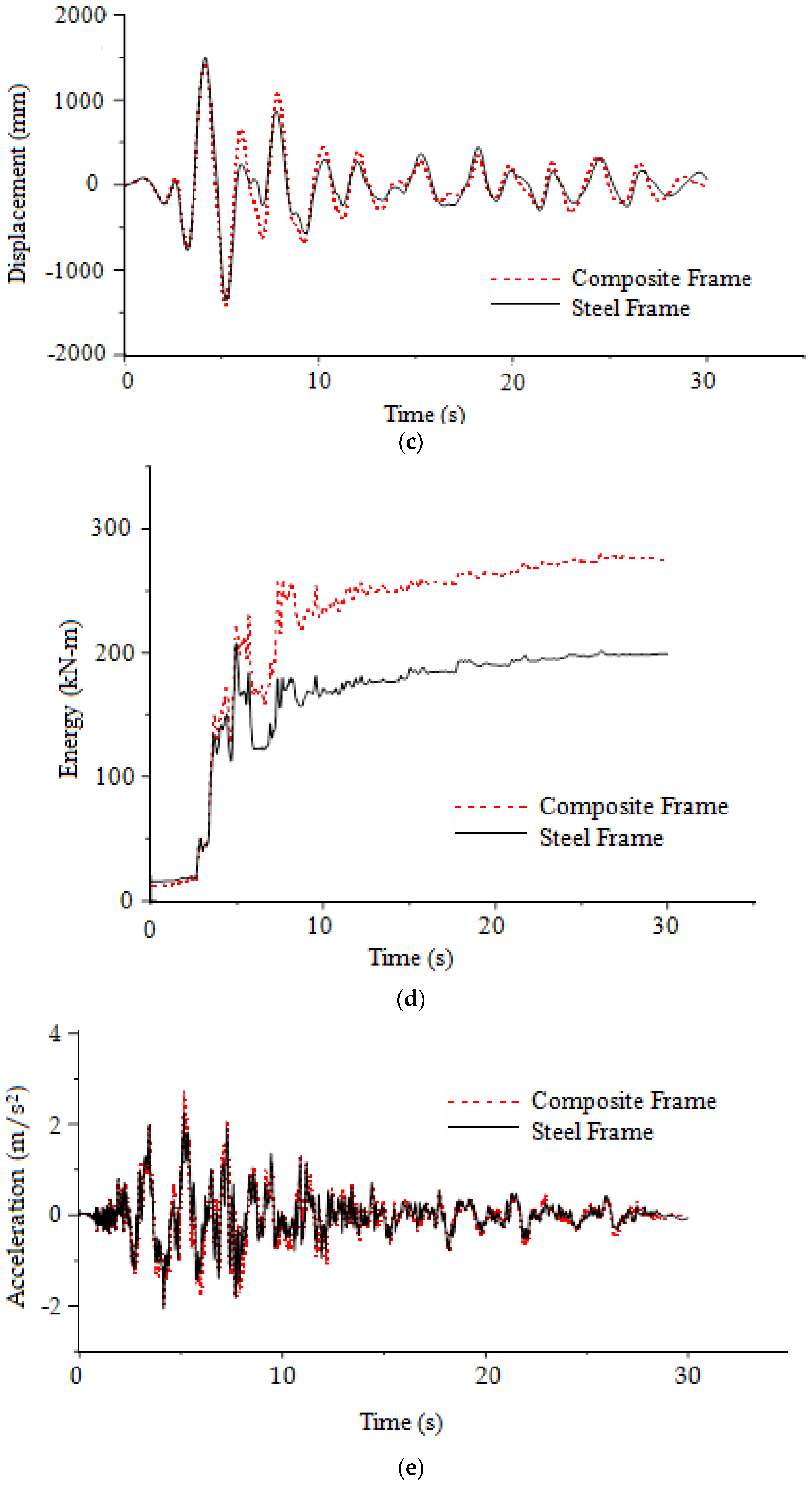
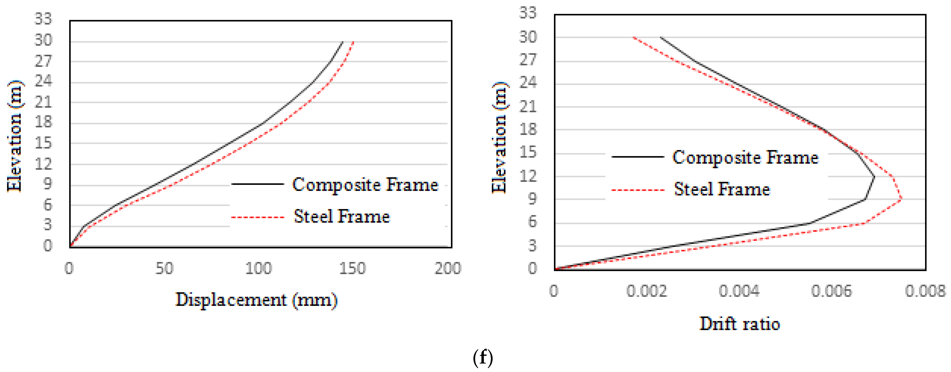
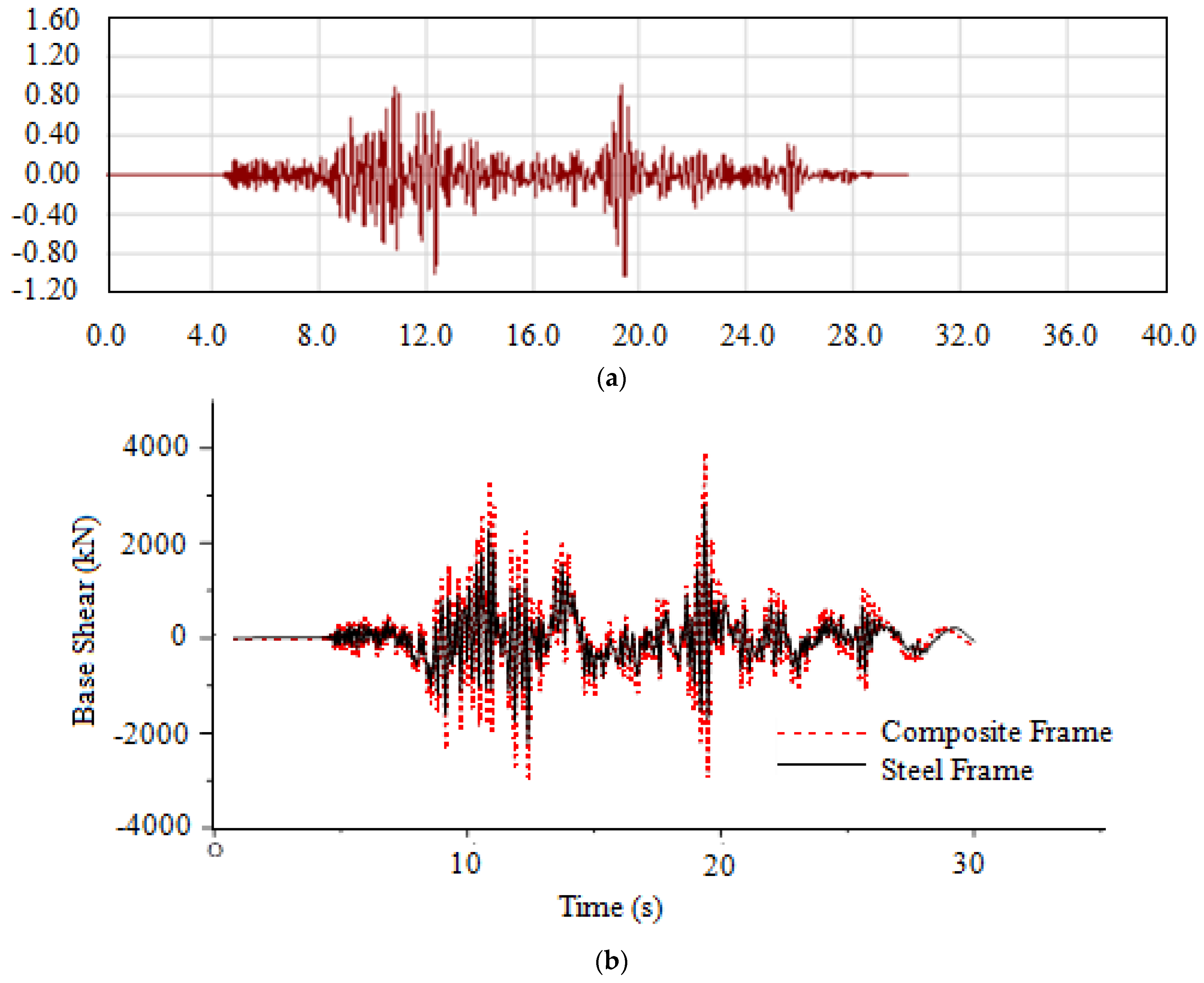
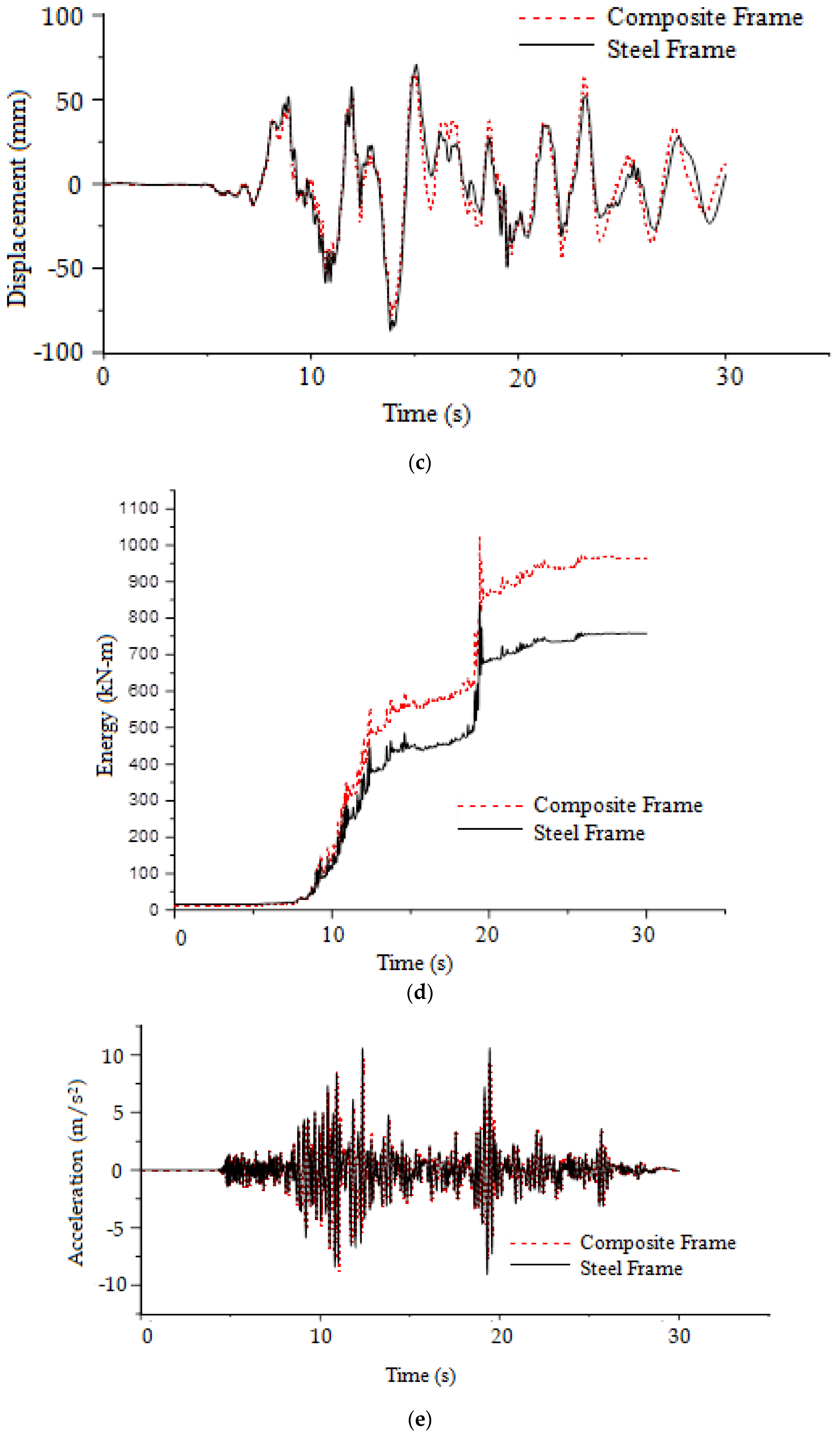
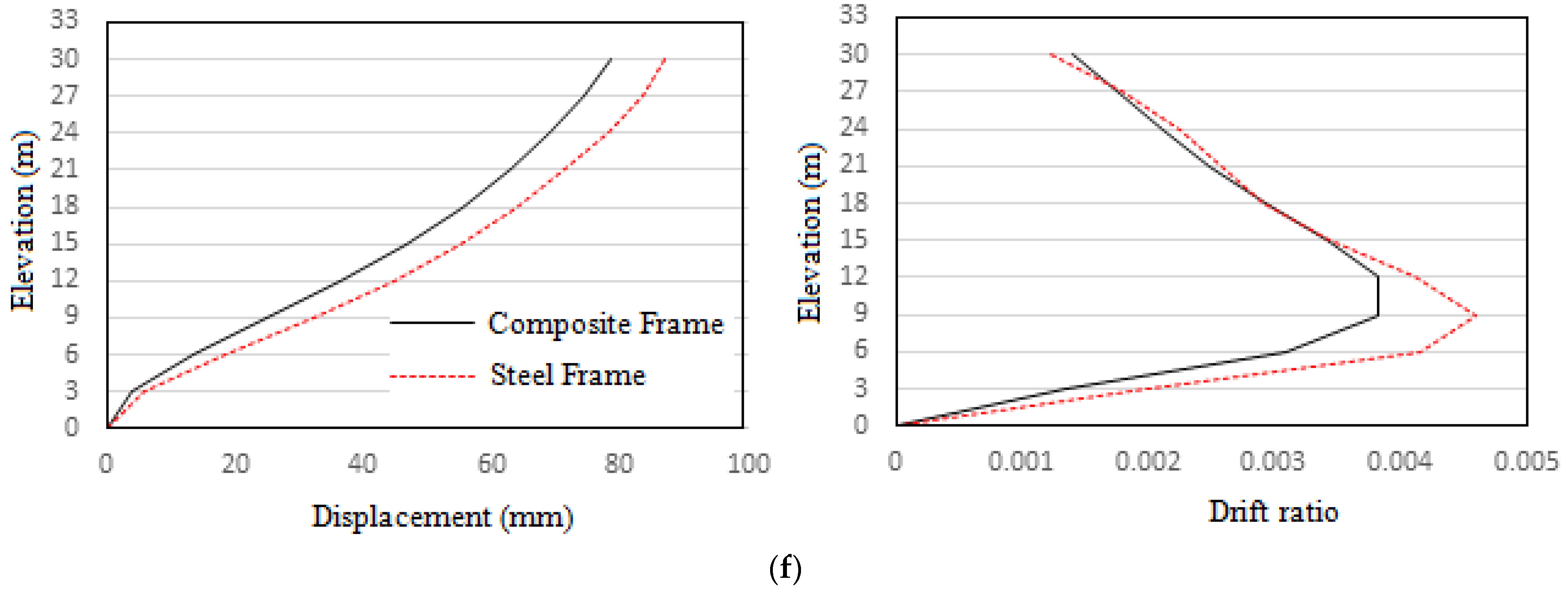
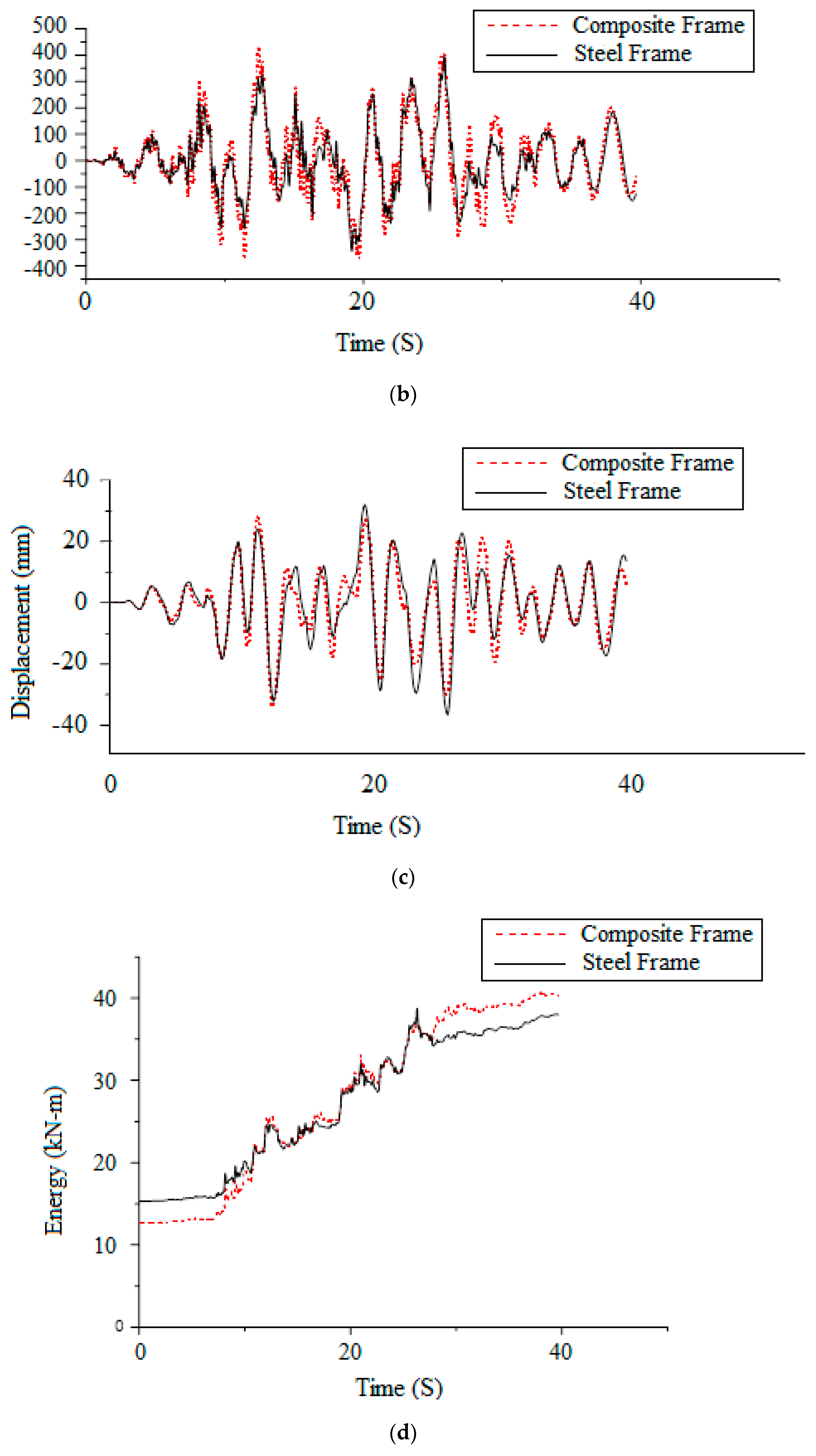
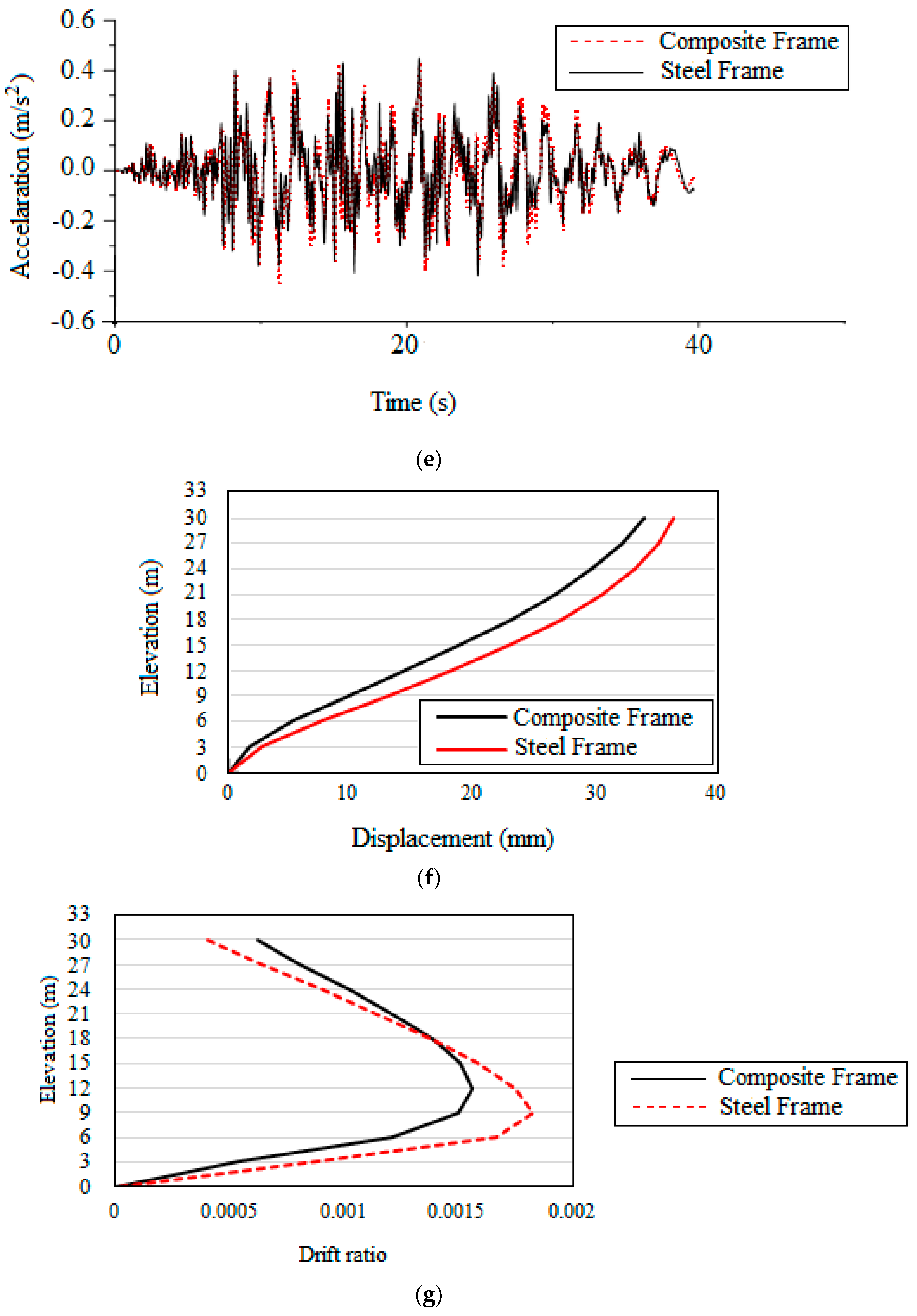
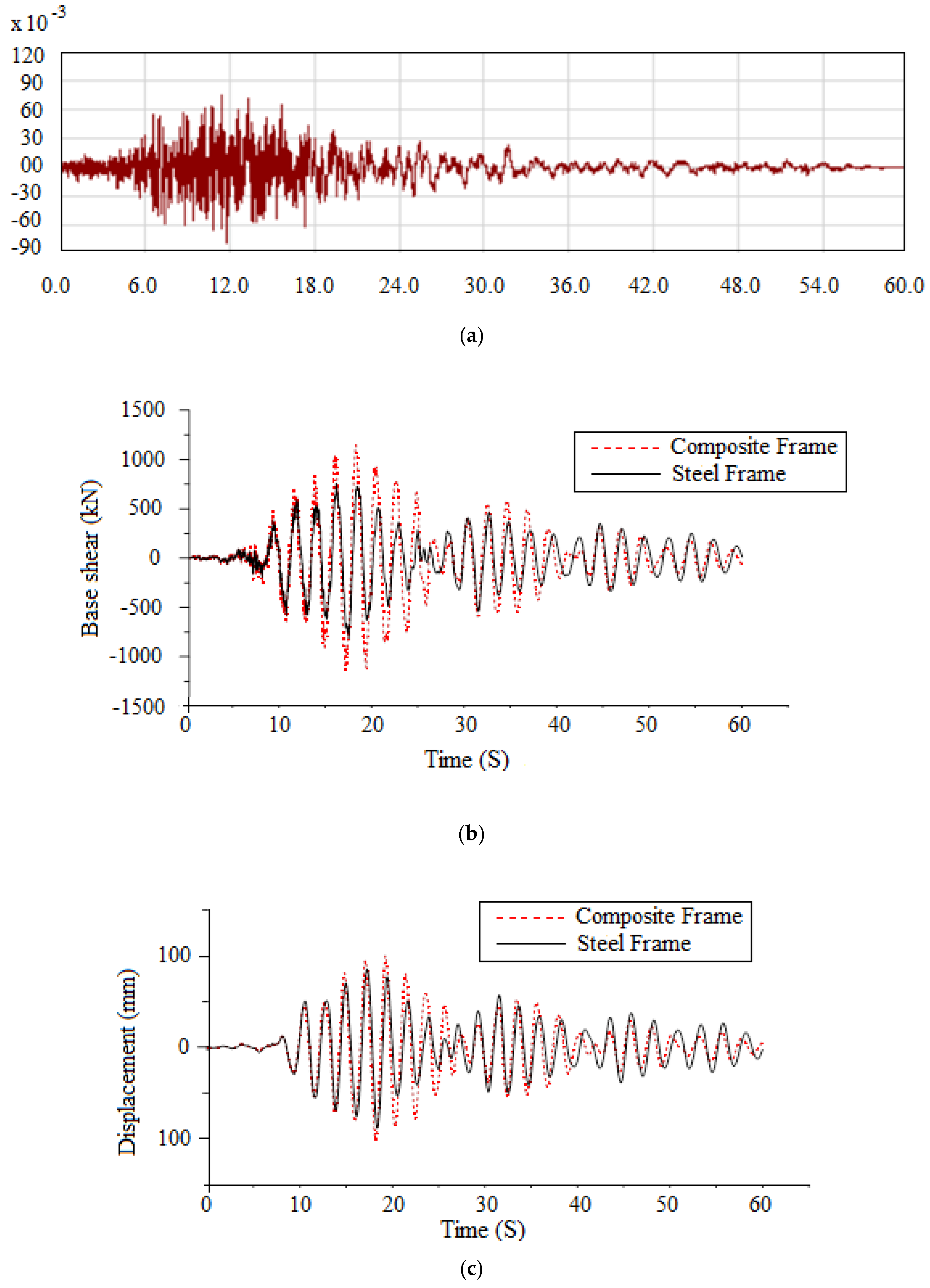
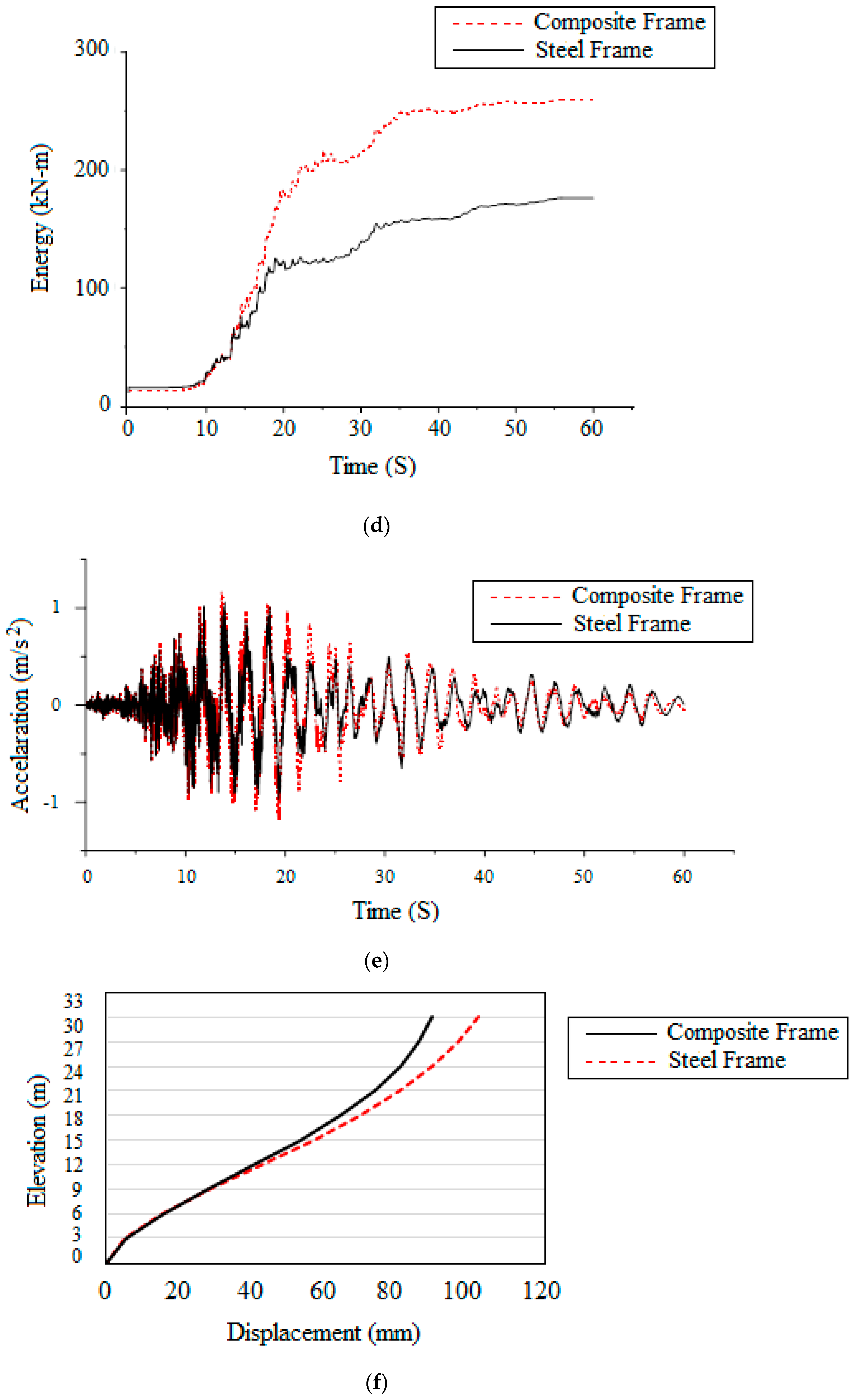
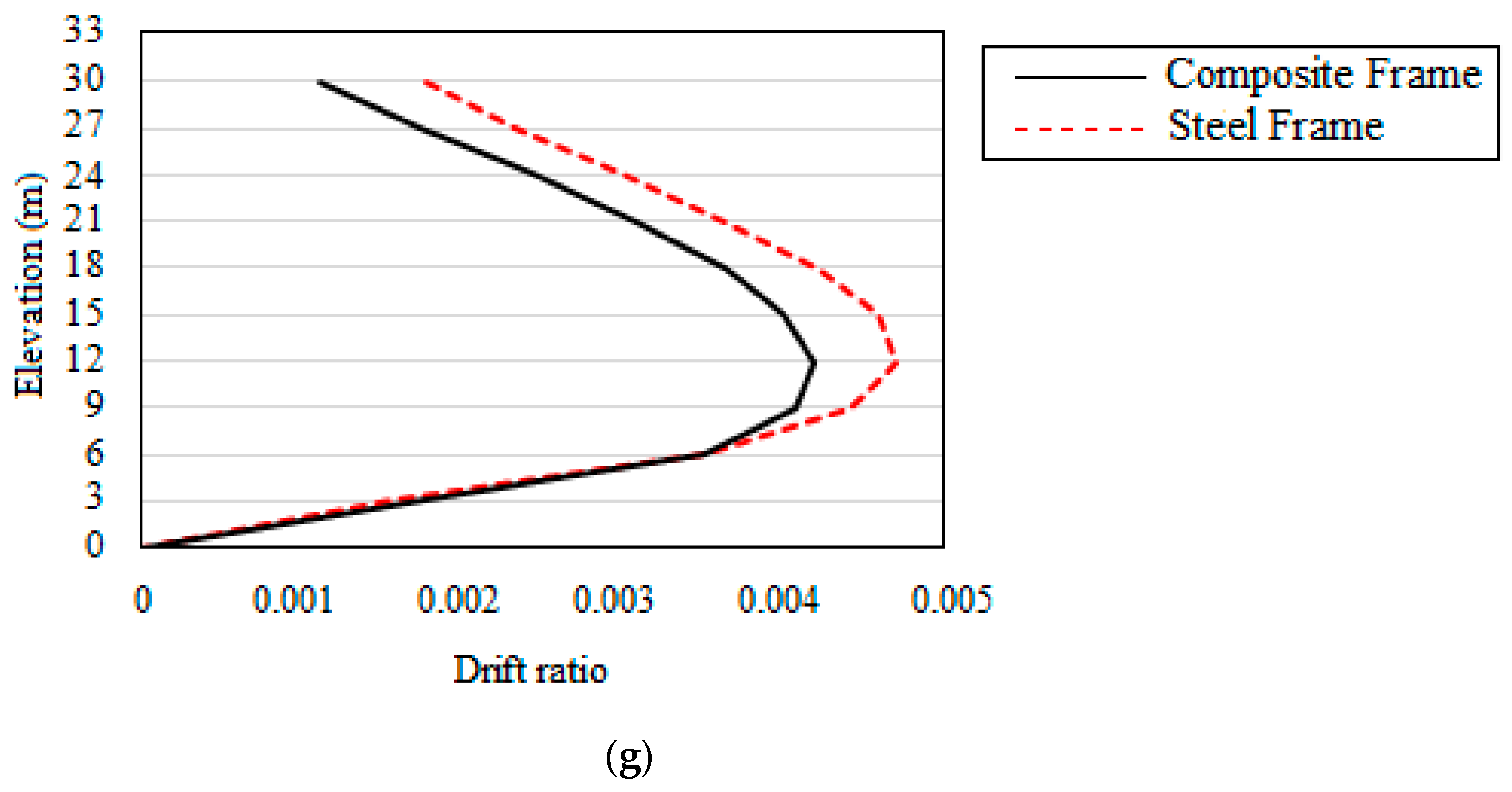
4.10. Comparison of Earthquake Responses
4.11. Comparison of Column Hinge C6H1 at Base Story
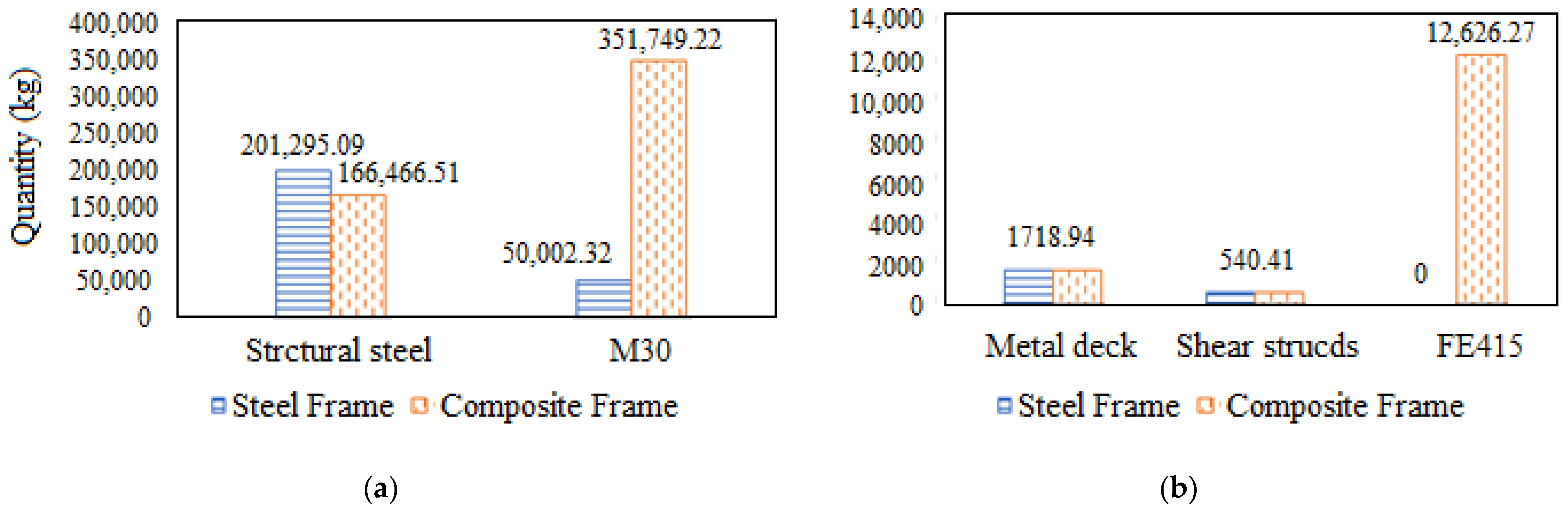
4.12. Quantity of Materials Comparison
5. Conclusions
- The results from response spectrum analysis show that the displacements and drifts are greater in steel frames, and the responses such as story shears, overturning moments, and story stiffness are greater in composite frames;
- From the idealized capacity curve, the stiffness of the composite frame is 21.5% higher in the elastic region and 41.2% higher in the nonlinear region initially, and 5.5% higher when nearing collapse than that of the steel frame;
- The ductility ratio of the composite frame is 2.75, and that of the steel frame is 2.56. The lateral strength of the composite frame from the idealized capacity curve is 4414.6 kN, and that of the steel frame is 3432.5 kN. Furthermore, the maximum base shear value in the composite frame is 22.3% higher than that of the steel frame;
- The steel frame has an 8.4% higher story drift than the composite frame;
- The performance points using the capacity spectrum method for steel and composite frames as per IS1893:2002 are (2875.25 kN, 320.74 mm) and (3733.57, 312.26 mm), respectively, for the design-based earthquake (DBE);
- The target displacement points using the displacement coefficient method for steel and composite frames as per IS1893:2002 are (2954.46 kN, 344.01 mm) and (3787.86 kN, 322.69 mm), respectively, for a design-based earthquake (DBE);
- From time history analysis, it is concluded that the displacement and drift values are found to be more dependent on the frequency of the earthquakes and how close they are to the natural frequency of the frames due to the effect of resonance. The closer the frequencies, the greater the response;
- The composite frame requires 21% less structural steel compared to the steel frame and 85% more concrete compared to the steel frame. In addition, the composite frame requires 6% more steel for the Fe415 rebars.
Author Contributions
Funding
Data Availability Statement
Conflicts of Interest
References
- Whittaker, A.; Constantnou, M.; Tsopelas, P. Displacement Estimates for Performance Based Seismic Design. J. Struct. Div. ASCE 1998, 124, 905–912. [Google Scholar] [CrossRef]
- Architectural Institute of Japan (AIJ). Structural Calculations of Steel Reinforced Concrete Structures; Architectural Institute of Japan (AIJ): Tokyo, Japan, 1987. [Google Scholar]
- American Institute of Steel Construction (AISC). Load and Resistance Factor Design Specification for Structural Steel Buildings; AISC: Chicago, IL, USA, 1999. [Google Scholar]
- Ghobarah, A.; Abou-Elfath, H.; Biddah, A. Response-Based Damage Assessment of Structures. Earthq. Eng. Eng. Seismol. 1999, 28, 79–104. [Google Scholar] [CrossRef]
- Chopra, A.K.; Chintanapakdee, C. Comparing response of SDF Systems to Near-Fault and Far-Fault Earthquake Motions in the Context of Spectral Regions. Earthq. Eng. Struct. Dyn. 2001, 30, 1769–1789. [Google Scholar] [CrossRef]
- Xue, Q. A Direct Displacement Based Seismic Design Procedure of Inelastic Structures. Eng. Struct. 2001, 23, 1453–1460. [Google Scholar] [CrossRef]
- Elenas, A.; Meskouris, K. Correlation study between seismic acceleration parameters and damage indices of structures. Eng. Struct. 2001, 23, 698–704. [Google Scholar] [CrossRef]
- IS 1893; Indian Code for Earthquake Resistant Structures. Bureau of Indian Standards: New Delhi, India, 2002.
- IS 12778; Indian Standard Code of Practice for Hot Rolled Parallel Flange Steel Sections for Beams, Columns and Bearing Piles—Dimensions and Section Properties. Bureau of Indian Standards: New Delhi, India, 2004.
- Oh, M.; Ju, Y.; Kim, M.; Kim, S. Structural Performance of Steel-Concrete Composite Column Subjected to Axial and Flexural Loading. J. Asian Archit. Build. Eng. 2006, 5, 153–160. [Google Scholar] [CrossRef]
- IS 800; Indian Standard Code of Practice for General Construction in Steel. Bureau of Indian Standards: New Delhi, India, 2007.
- Mohd, Y.A.Y.; David, A.N. Cross-sectional properties of complex composite beams. Eng. Struct. 2007, 29, 195–212. [Google Scholar] [CrossRef]
- Gewei, Z.; Basu, B. A study on friction-tuned mass damper: Harmonic solution and statistical linearization. J. Vib. Control 2010, 17, 721–731. [Google Scholar] [CrossRef]
- Sayani, P.J.; Erduran, E.; Ryan, K.L. Comparative response assessment of minimally compliant low-rise base isolated and conventional steel moment resisting frame buildings. J. Struct. Eng. ASCE 2011, 137, 1118–1131. [Google Scholar] [CrossRef]
- Gray, B.M.; Christopoulos, C.; Eng, P.; Packer, J.; Gray, M. A New Brace Option for Ductile Braced Frames. Mod. Steel Constr. 2012, 40–43. Available online: https://www.aisc.org/globalassets/modern-steel/archives/2012/02/2012v02_new_brace.pdf (accessed on 5 July 2023).
- Wankhade, R.L.; Landage, A.B. Static Analysis For Fixed Base And Base Isolated Building Frame. In Proceedings of the National Conference on Advances in Civil and Structural Engineering (NCACSE-2014), Karad, India, 18–19 April 2014. [Google Scholar]
- Wankhade, R.L. Performance Based Design and Estimation of Forces for Building Frames with Earthquake Loading. In Proceedings of the International Conference on Recent Trends and Challenges in Civil Engineering, Allahabad, India, 12–14 December 2014; MNNIT Allahabad: Allahabad, India, 2014. [Google Scholar]
- Wankhade, R.L.; Landage, A.B. Performance Based Analysis and Design of Building Frames with Earthquake Loading. Int. J. Eng. Res. 2016, 5, 106–110. [Google Scholar]
- Wankhade, R.L. Performance Analysis of RC Moment Resisting Frames Using Different Rubber Bearing Base Isolation Techniques. In Proceedings of the International Conference on Innovations in Concrete for Infrastructure Challenges, Nagpur, India, 6–7 October 2017. [Google Scholar]
- Titikesh, A.; Bhatt, G. Optimum positioning of shear walls for minimizing the effects of lateral forces in multistorey buildings. Arch. Civ. Eng. 2017, 63, 151–162. [Google Scholar] [CrossRef]
- Bazarchi, E.; Hosseinzadeh, Y.; Panjebashi, A.P. Investigating the in-plane flexibility of steel-deck composite floors in steel structures. Int. J. Struct. Integr. 2018, 9, 705–720. [Google Scholar] [CrossRef]
- Boukhalkhal, S.H.; Jhaddoudene, A.N.T.; Neves, L.F.D.C.; de Silva, V.P.C.G.; Madi, W. Performance assessment of steel structures with semi-rigid joints in seismic areas. Int. J. Struct. Integr. 2019, 11, 13–28. [Google Scholar]
- Nayak, C.B.; Jagadale, U.T.; Jadhav, K.M.; Morkhade, S.G.; Kate, G.K.; Thakare, S.B.; Wankhade, R.L. Experimental, analytical and numerical performance of RC beams with V-shaped reinforcement. Innov. Infrastruct. Solut. 2021, 6, 2. [Google Scholar] [CrossRef]
- Wankhade, R.L.; Sawarkar, A.; Chandwani, A.; Chavan, S.; Malkar, P.; Sawarkar, G. Seismic Fragility of Buildings Subjected to Pounding Effects with Soil–Structure Interaction. In Advances in Construction Materials and Sustainable Environment; Gupta, A.K., Shukla, S.K., Azamathulla, H., Eds.; Lecture Notes in Civil Engineering; Springer: Singapore, 2022; Volume 196. [Google Scholar] [CrossRef]
- Miani, M.; Di Marco, C.; Frappa, G.; Pauletta, M. Effects of Dissipative Systems on the Seismic Behavior of Irregular Buildings–Two Case Studies. Buildings 2020, 10, 202. [Google Scholar] [CrossRef]
- Frappa, G.; Pauletta, M. Seismic retrofitting of a reinforced concrete building with strongly different stiffness in the main directions. In Proceedings of the 14th fib International Ph.D. Symposium in Civil Engineering, Rome, Italy, 5–7 September 2022. [Google Scholar]
- Mo, Z.; Feng, Q.; Lai, B.; Jiang, W.; Feng, Y. Resilient performance of super-elastic SMA bolted connection equipped with extended end plate and shear tab. J. Constr. Steel Res. 2022, 199, 107626. [Google Scholar] [CrossRef]
- Lai, B.; Tan, W.; Feng, Q.; Venkateshwaran, A. Numerical parametric study on the uniaxial and biaxial compressive behavior of H-shaped steel reinforced concrete composite beam-columns. Adv. Struct. Eng. 2022, 25, 2641–2661. [Google Scholar] [CrossRef]


| Object | Section | Plastic Moment Capacity, Mp (kN-m) | |
|---|---|---|---|
| Column (IS 12778:2004) | Steel | WPB 300 × 300 (237.92 kg/m) | 1406.84 |
| Composite | WPB 360 × 370 (165.34 kg/m) Embedded cross section | 1407.27 | |
| Primary beam for both frames (IS 800:2007) | ISWB 300 (48.1 kg/m) | 182.80 | |
| Secondary beam for both frames (IS 800:2007) | ISLB 225 (23.5 kg/m) | 63.68 | |
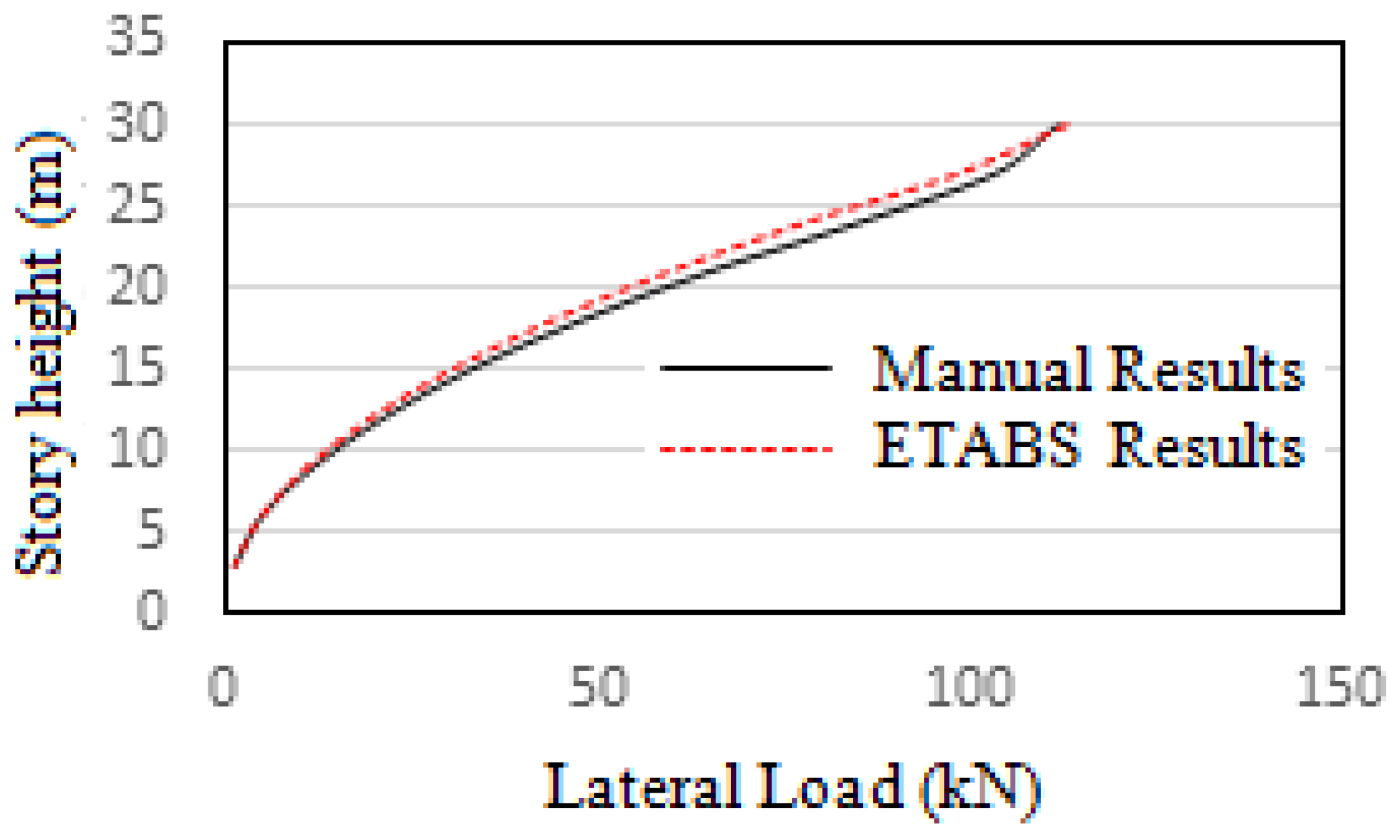
| Story | Elevation (m) | Lateral Load Distribution (kN) | |
|---|---|---|---|
| Software | Manual | ||
| Story10 | 30 | 112.9491 | 111.799 |
| Story9 | 27 | 98.3869 | 103.4 |
| Story8 | 24 | 77.7378 | 85.2 |
| Story7 | 21 | 59.518 | 65.01 |
| Story6 | 18 | 43.7275 | 47.77 |
| Story5 | 15 | 30.3663 | 32.99 |
| Story4 | 12 | 19.4344 | 21.17 |
| Story3 | 9 | 10.9319 | 11.82 |
| Story2 | 6 | 4.8586 | 4.925 |
| Story1 | 3 | 1.2147 | 1.329 |
| Ʃ Total | 459.14 | 492.51 | |
| Mode | Period(s) | |
|---|---|---|
| Composite | Steel | |
| 1 | 2.189 | 2.373 |
| 2 | 2.187 | 2.339 |
| 3 | 1.775 | 2.001 |
| Response | RSx | RSy | ||
|---|---|---|---|---|
| Composite | Steel | Composite | Steel | |
| Maximum story displacement (mm) | 41.17 | 43.43 | 41.21 | 43.96 |
| Maximum story drift | 0.0019 | 0.00214 | 0.0019 | 0.00216 |
| Story overturning moment (kN-m) | 9550.4 | 8195.9 | 9541.2 | 8046.4 |
| Story shear (kN) | 533.39 | 444.41 | 532.98 | 437.02 |
| Story stiffness (kN/mm) | 259.8 | 142.7 | 259.6 | 140.3 |
| Step | Monitored Displ. (mm) | Base Force (kN) | A-B | B-C | C-D | D-E | >E | A-IO | IO-LS | LS-CP | >CP | Total |
|---|---|---|---|---|---|---|---|---|---|---|---|---|
| 0 | 0 | 0 | 800 | 0 | 0 | 0 | 0 | 800 | 0 | 0 | 0 | 800 |
| 1 | 120 | 1345.5072 | 800 | 0 | 0 | 0 | 0 | 800 | 0 | 0 | 0 | 800 |
| 2 | 194.075 | 2176.0667 | 798 | 2 | 0 | 0 | 0 | 800 | 0 | 0 | 0 | 800 |
| 3 | 244.108 | 2614.2609 | 736 | 64 | 0 | 0 | 0 | 776 | 24 | 0 | 0 | 800 |
| 4 | 368.062 | 3036.3915 | 678 | 122 | 0 | 0 | 0 | 690 | 110 | 0 | 0 | 800 |
| 5 | 550.505 | 3395.5062 | 654 | 146 | 0 | 0 | 0 | 656 | 114 | 30 | 0 | 800 |
| 6 | 572.011 | 3432.5150 | 652 | 146 | 2 | 0 | 0 | 656 | 96 | 48 | 0 | 800 |
| 7 | 563.901 | 3117.8298 | 652 | 136 | 4 | 0 | 8 | 656 | 94 | 42 | 8 | 800 |
| Step | Monitored Displ. (mm) | Base Force (kN) | A-B | B-C | C-D | D-E | >E | A-IO | IO-LS | LS-CP | >CP | Total |
|---|---|---|---|---|---|---|---|---|---|---|---|---|
| 0 | 0 | 0 | 800 | 0 | 0 | 0 | 0 | 800 | 0 | 0 | 0 | 800 |
| 1 | 120 | 1713.0875 | 800 | 0 | 0 | 0 | 0 | 800 | 0 | 0 | 0 | 800 |
| 2 | 204.016 | 2884.5333 | 796 | 4 | 0 | 0 | 0 | 800 | 0 | 0 | 0 | 800 |
| 3 | 256.971 | 3445.6811 | 716 | 84 | 0 | 0 | 0 | 768 | 32 | 0 | 0 | 800 |
| 4 | 378.584 | 4078.8834 | 650 | 150 | 0 | 0 | 0 | 680 | 120 | 0 | 0 | 800 |
| 5 | 472.306 | 4378.2101 | 618 | 182 | 0 | 0 | 0 | 646 | 154 | 0 | 0 | 800 |
| 6 | 525.33 | 4455.5615 | 616 | 184 | 0 | 0 | 0 | 636 | 164 | 0 | 0 | 800 |
| 7 | 549.436 | 4473.9862 | 616 | 184 | 0 | 0 | 0 | 624 | 172 | 4 | 0 | 800 |
| 8 | 596.002 | 4430.5584 | 614 | 174 | 0 | 0 | 12 | 616 | 146 | 38 | 0 | 800 |
| 9 | 605.241 | 4414.625 | 612 | 176 | 0 | 0 | 12 | 616 | 128 | 56 | 0 | 800 |
| 10 | 614.824 | 4376.4091 | 612 | 176 | 0 | 0 | 12 | 616 | 122 | 62 | 0 | 800 |
| 11 | 620.741 | 4327.1105 | 612 | 172 | 0 | 0 | 16 | 616 | 120 | 64 | 0 | 800 |
| 12 | 620.753 | 4327.1298 | 612 | 172 | 0 | 0 | 16 | 616 | 120 | 64 | 0 | 800 |
| 13 | 628.401 | 4259.8434 | 612 | 172 | 0 | 0 | 16 | 616 | 108 | 76 | 0 | 800 |
| 14 | 631.331 | 4243.5798 | 612 | 168 | 4 | 0 | 16 | 616 | 106 | 78 | 0 | 800 |
| 15 | 631.343 | 4061.4931 | 612 | 164 | 2 | 0 | 22 | 616 | 104 | 74 | 6 | 800 |
| 16 | 633.795 | 4078.3067 | 612 | 162 | 4 | 0 | 22 | 616 | 104 | 74 | 6 | 800 |
| Parameters | Performance Point as per FEMA 440 EL | |
|---|---|---|
| Composite Frame | Steel Frame | |
| Shear (kN) | 3733.57 | 2875.25 |
| Displacement (mm) | 312.26 | 320.74 |
| Sa (g) | 0.1886 | 0.1568 |
| Sd (mm) | 242.25 | 257.97 |
| Teff (s) | 2.18 | 2.39 |
| Parameters | Target Displacement as per ASCE 41-13 NSP | |
|---|---|---|
| Composite Frame | Steel Frame | |
| Shear (kN) | 3787.86 | 2954.46 |
| Displacement (mm) | 322.69 | 344.01 |
| Region | Ideal Curve Composite | Ideal Curve Steel | ||
|---|---|---|---|---|
| Displacement (mm) | Base Shear (kN) | Displacement (mm) | Base Shear (kN) | |
| Elastic region | 0 | 0 | 0 | 0 |
| 220.009 | 3140.79 | 223.709 | 2508.351 | |
| Plastic region | 322.69 | 3787.862 | 344.005 | 2954.464 |
| 605.241 | 4414.625 | 572.011 | 3432.515 | |
| Hinge Number | Frame | Moment, M3 (kN-m) | Hinge State | Hinge Level | Rotation (rad) |
|---|---|---|---|---|---|
| B14H18 | Composite | 201.3 | B to ≤C | LS to ≤CP | 0.027 |
| Steel | 0 | >E | >CP | 0.047 |
| Hinge Number | Frame | Moment, M3 (kN-m) | Hinge State | Hinge Level | Rotation (rad) | Axial Force (kN) |
|---|---|---|---|---|---|---|
| C9H17 | Composite | 547.5 | A to ≤B | A to ≤IO | 0.0008 | 547.5 |
| Steel | 463.4 | A to ≤B | A to ≤IO | 0 | 463.4 |
| Hinge Number | Frame | Moment, M3 (kN-m) | Hinge State | Hinge Level | Rotation (rad) | Axial Force (kN) |
|---|---|---|---|---|---|---|
| C6H1 | Composite | 1761.5 | B to ≤C | LS to ≤CP | 0.0067 | 1409.5 |
| Steel | 1317.4 | A to ≤B | A to ≤IO | 0 | 1217.1 |
| Earthquake Name | Year | Station Name | Mechanism | Type | Magnitude Mw | Epicentral Distance Rrup (km) | Vs (m/s) |
|---|---|---|---|---|---|---|---|
| Kocaeli, Turkey | 1999 | Izmit | Strike-Slip | Near-Field | 7.51 | 7.21 | 811 |
| Duzce, Turkey | 1999 | IRIGM496 | Strike-Slip | Near-Field | 7.14 | 7.14 | 760 |
| Landers | 1992 | Palm Springs Airport | Strike-Slip | Far-Field | 7.28 | 159.13 | 315.06 |
| Big Bear-01 | 1992 | LA-NWestmoreland | Strike-Slip | Far-Field | 6.46 | 51.51 | 312.47 |
| Event | Frame Type | Top Story Displacement (mm) | Drift Ratio | Base Shear (kN) | Joint Acceleration (m/s2) | Energy (kN-m) |
|---|---|---|---|---|---|---|
| Kocaeli (Near-field) | Composite | 144.54 | 0.0069 | 1837.8 | 2.75 | 279.16 |
| Steel | 150.38 | 0.0075 | 1488.35 | 2.26 | 207.94 | |
| Duzce (Near-field) | Composite | 78.60 | 0.0038 | 3943.91 | 10.55 | 1022.11 |
| Steel | 87.08 | 0.0046 | 2819.54 | 10.61 | 836.73 | |
| Landers (Far-field) | Composite | 34.21 | 0.0016 | 434.48 | 0.449 | 40.68 |
| Steel | 36.59 | 0.0018 | 395.13 | 0.445 | 38.77 | |
| Big Bear (Far-field) | Composite | 101.37 | 0.0047 | 1145.46 | 1.18 | 259.80 |
| Steel | 88.86 | 0.0042 | 816.76 | 1.06 | 176.35 |
| Event | Frame Type | Moment, M3 (kN-m) | Rotation, Φ (rad) | Axial Force, P (kN) | Hinge Level |
|---|---|---|---|---|---|
| Duzce (Near-field) | Composite | 568.65 | 0.00078 | 1414.54 | A to ≤IO |
| Steel | 403.58 | 0 | 1234.40 | A to ≤IO | |
| Kocaeli (Near-field) | Composite | 548.78 | 0.00074 | 1408.62 | A to ≤IO |
| Steel | 357.35 | 0 | 1216.73 | A to ≤IO | |
| Landers (Far-field) | Composite | 123.48 | 0.00013 | 1413.29 | A to ≤IO |
| Steel | 91.87 | 0 | 1235.60 | A to ≤IO | |
| Big Bear (Far-field) | Composite | 353.31 | 0.0039 | 1414.70 | A to ≤IO |
| Steel | 187.25 | 0 | 1223.38 | A to ≤IO |
| Materials | Quantity (kg) | |
|---|---|---|
| Composite | Steel | |
| Structural steel | 166,466.51 | 201,295.09 |
| M30 | 351,749.22 | 50,002.32 |
| Metal deck | 1718.94 | 1718.94 |
| Shear studs | 540.41 | 540.41 |
| Fe 415 | 12,626.27 | 0 |
Disclaimer/Publisher’s Note: The statements, opinions and data contained in all publications are solely those of the individual author(s) and contributor(s) and not of MDPI and/or the editor(s). MDPI and/or the editor(s) disclaim responsibility for any injury to people or property resulting from any ideas, methods, instructions or products referred to in the content. |
© 2023 by the authors. Licensee MDPI, Basel, Switzerland. This article is an open access article distributed under the terms and conditions of the Creative Commons Attribution (CC BY) license (https://creativecommons.org/licenses/by/4.0/).
Share and Cite
Gajbhiye, P.D.; Mashaan, N.S.; Bhaiya, V.; Wankhade, R.L.; Vishnu, S.P. Inelastic Behavior of Steel and Composite Frame Structure Subjected to Earthquake Loading. Appl. Mech. 2023, 4, 899-926. https://doi.org/10.3390/applmech4030047
Gajbhiye PD, Mashaan NS, Bhaiya V, Wankhade RL, Vishnu SP. Inelastic Behavior of Steel and Composite Frame Structure Subjected to Earthquake Loading. Applied Mechanics. 2023; 4(3):899-926. https://doi.org/10.3390/applmech4030047
Chicago/Turabian StyleGajbhiye, P. D., Nuha S. Mashaan, V. Bhaiya, Rajan L. Wankhade, and S. P. Vishnu. 2023. "Inelastic Behavior of Steel and Composite Frame Structure Subjected to Earthquake Loading" Applied Mechanics 4, no. 3: 899-926. https://doi.org/10.3390/applmech4030047