Article

Biomass Combustion in the Helically Coiled Domestic Boiler Combined with the Equilibrium/Chemical Kinetics CFD Approach

by
Izabela Wardach-Święcicka
,
Sylwia Polesek-Karczewska
* and
Dariusz Kardaś
The Szewalski Institute of Fluid-Flow Machinery, Polish Academy of Sciences, 80-231 Gdansk, Poland
*
Author to whom correspondence should be addressed.
Appl. Mech. 2023, 4(2), 779-802; https://doi.org/10.3390/applmech4020040
Submission received: 28 February 2023 / Revised: 9 May 2023 / Accepted: 6 June 2023 / Published: 17 June 2023
(This article belongs to the Special Issue Applied Thermodynamics: Modern Developments (2nd Volume))

Abstract

:
In the face of threats related to energy supply and climate change, the use of biomass is gaining importance, particularly in distributed energy systems. Combustion of biomass, including residue biomass, is considered one of the routes to increase the share of renewables in energy generation. The modeling of gaseous phase reactions remains crucial in predicting the combustion behavior of biomass and pollutant emissions. However, their simulation becomes a challenging task due to the computational cost. This paper presents a numerical analysis of the combustion process of a gas mixture released during biomass decomposition in a domestic 25 kW coil-type boiler. Three types of biogenic fuels were taken into consideration. The work aimed at examining the available tools for modeling gas burning, thus the geometry of the system was limited only to the 2D case. The thermodynamic equilibrium composition of pyrolysis gas was determined and implemented in Ansys to simulate the process. The computational results showed the potential of detailed, but reduced, combustion mechanisms of CH 4 / CO / H 2 mixtures in predicting the main process features. The mechanism involving 85 reactions appeared to be more reliable compared to that comprising 77 reactions, particularly for volatiles with higher H 2 content, whilst offering an acceptable calculation time. The burning characteristics obtained for volatiles with less CH 4 and more H 2 are in good agreement with the real operation conditions reported for the boiler.

1. Introduction

In the last decades, the global trends targeted at reducing the carbon footprint and mitigating global warming by eliminating the use of fossil fuels in the energy sector have attracted increased interest in the utilization of biomass [1], which is considered a CO 2 neutral resource. Along with this, considering the biomass potential in heat and power generation and the production of biofuels, efforts have intensified towards the use of locally available biomass of a different kind. Combustion of biomass, besides geothermal energy and hydropower, is a necessary complement to increasing the development of solar and wind energy, due to their predictability, and ability to secure the energy supply [2]. As it has been forecasted by the International Energy Agency, by 2050, combustion of biomass may reach as high as 50% of the global heating demand [3]. The use of biomass for energy purposes involves both large-scale heat and power generation [4,5,6] and small-scale units [7,8,9]. Particularly, low-grade fuels are now considered an alternative to fossil fuels as a relatively cheap energy source [10,11]. Despite the carbon neutrality benefits, biomass combustion technology must face technical and environmental challenges related to particulate matter emissions that are strongly linked to biomass fuel characteristics. Biomass has far higher volatile content compared to coal, which translates into more rapid fuel burning that may cause the release of fine unburned and ash particles into the atmosphere. Due to the high contents of alkali metals (mainly sodium and potassium) in biomass fuels, the ash deposits lead to slagging and fouling problems [4,12] that eventually lead to the deterioration of heating surfaces and lowering heat transfer rates [13,14]. The slagging and fouling tendencies are facilitated by the presence of chlorine, which contributes to the potassium transfer in the gas phase and to further chemical reactions, and this is considered to eventually initiate corrosion [15,16].
These aforementioned issues strongly affect the efficiency and maintenance of boilers and furnaces [17]. The utilization of low-cost biomass resources may improve the pro-ecological balance of the energy sector. However, biomass properties that are strongly dependent on the fuel origin are reported to significantly affect the performance of boilers. In particular, this refers to alternative fuels of lower quality, e.g., agriculture residues. Their burning in small-scale units leads to slagging problems and increased emission levels [8]. The technical and environmental aspects are related not only to the fuel’s physicochemical composition, but also to the operation and design of a device. Meanwhile, small-scale boilers available on the market are designed for specific types of fuels, e.g., woody (pellets or chips) or non-woody fuels [9]. The further development of biomass combustion technology should therefore follow the demand for efficient and low-emission domestic combustion systems, and additionally should be highly flexible in fuel type [18,19].
The control of biomass combustion and the prevention of technical problems related to the process route and resulting contaminants, requires in-depth knowledge of the chemical behavior of the fuel components and the burning products [20,21]. Computational fluid dynamics (CFD) packages appear to be a reliable and cost-effective tool to better understand, predict, and optimize biomass combustion units. CFD packages provide the opportunity to analyze the systems for a variety of parameters and operational conditions, and to find ways to reduce the time- and cost-demanding empirical investigations; they have become a valuable support in the system development [22]. Nevertheless, solid fuel combustion is of a complex nature and its mathematical description involves a number of issues, including fluid dynamics, heat and mass transfer, phase transitions, and chemical kinetics. It begins with fuel drying, which is followed by devolatilization, and then by homogeneous and heterogeneous (char–gas) chemical reactions. The multiphase nature of combustion is usually described by decoupling the equations for gas and particles, wherein the solution for the gaseous phase utilizes the Eulerian approach, and the solution for the solid phase uses the Eulerian–Lagrangian type approach adopting the discrete phase model (DPM) or discrete element method (DEM) [23,24,25]. The accurate description of chemical routes is vital for the overall process characteristics. The volatiles released during fuel thermal decomposition as a mixture of CO, CO 2 , H 2 O , CH 4 , H 2 , and higher hydrocarbons, are the source for homogeneous combustion. Devolatilization, due to its extreme complexity, is usually described using global kinetics. These include the simplest models that allow for the accurate prediction of gas yield rates and more complex ones that are successful in determining the pyrolysis gas composition [25,26]. Furthermore, with regards to the homogeneous reactions, various approaches are considered that include the use of various types of reaction mechanisms. Highly detailed reaction mechanisms, involving hundreds of chemical species and the reactions they take part in, are offered by mechanisms of GRI-Mech [27] or San Diego [28]. However, since reactions in the gaseous phase are reported to consume most of the computational time [29], efforts are carried out to possibly simplify the reaction models while preserving reliable predictions of the key combustion products of interest. One of the simplest is the global one-step reaction that assumes pyrolysis gas to be described by the general lumped form of CH y O x and that no intermediate species is to be formed [26]. A two-step mechanism using two lumped species to represent the volatiles with CO as an intermediate species, was also utilized [23]. An improvement in the accuracy of biomass volatile combustion was obtained using the four-step mechanism for the combustion of hydrocarbons [23].
Biomass combustion has been extensively studied over the last decades, especially with regards to modern small- and medium-scale cogeneration systems [30]. Similarly, the helically coiled heat exchangers are often considered in this area owing to their advantage, which is a large heat transfer area compacted in a relatively small volume [31]. However, the majority of studies are limited to the analysis of thermal and flow characteristics inside the coiled tube [32,33,34]. The analyses of the detailed mechanisms of biomass volatile combustion are not numerous. Since they are of importance for the development of distributed renewable energy systems, the mathematical models involved in designing boilers should be cost-effective in terms of calculation time. Considering the significance of the gaseous phase reaction modeling to the prediction of biomass combustion characteristics, the present study aims to analyze different available detailed mechanisms of pyrolysis gas combustion that may be suitable for the implementation in the simulation of biomass combustion in a helically coiled domestic boiler with a 25 kW capacity. Using reliable and accurate predictions, this study simultaneously uses time-effective computation with a focus on the reduced reaction mechanisms. The proposed modeling approach involves the thermodynamic equilibrium to determine the composition of biomass volatiles as the input data for the 2D CFD computation, thereby eliminating the need for the detailed analysis of thermal and flow processes in the burner. The gas composition has been determined based on the outputs of the developed in-house numerical code that utilizes the Gibbs function minimization method coupled with the experimentally derived devolatilization data (from a thermogravimetric analysis). In this way, the approach offers the possibility to investigate the burning behavior of a wide spectrum of fuels in a reasonable amount of time. The effect of the initial pyrolysis gas composition on the burning behavior, including the distribution of temperature, velocity, and main reactant concentrations were studied and discussed.

2. Methodology—The Details of the CFD Analysis

The work is aimed to investigate the mechanism of gas combustion in a low-power coil-type boiler. Since the reaction mechanism is of interest in the analysis, the geometry of the system was simplified. Initially, the analysis was limited only to the part where the cooling of exhaust gases takes place first, i.e., the so-called small coil; then, the entire flue gas circulation space was modeled in a 2d simulation.
The scope of the work included: (i) the selection of the type of biomass; (ii) the determination of the pyrolysis gas composition for the considered types of biomass; (iii) the creation of the appropriate computational geometry; (iv) setting the initial and boundary conditions; (v) the selection of pyrolysis gas combustion mechanisms; and (vi) the CFD calculations using the Ansys FLUENT package and the analysis of the obtained results.

2.1. Geometry of the 25 kW Boiler

The computational domain was based on the actual dimensions of a 25 kW coiled tube boiler designed at the Institute of Fluid-Flow Machinery (IMP PAN), Gdańsk (Poland). The schematic of the real boiler is presented in Figure 1. The simplified 2D geometry of the boiler, including both the inner and outer coils used for the analysis of the gas-phase combustion process is demonstrated in Figure 2.
The simplified geometry enabled the reduction of the calculation domain to 84.5 k cells and the smallest diameter of a cell was around 4 mm.
For the numerical calculations, Ansys FLUENT software was used. To reduce the computation time, the steady axisymmetric cases were analyzed. Additionally, the standard turbulence k ϵ model, the species transport, and the reaction module were utilized.

2.2. Governing Equations

The general form of the mass conservation equation takes the form of [35]:
ρ t + · ρ u = S m ,
where S m is the mass added to the continuous phase.
Conservation of momentum is described by the equation:
t ρ u + · ρ u u = p + · τ + ρ g + F ,
where p is the static pressure, τ is the stress tensor, ρ g and F are the gravitational body force and external body forces, respectively.
The stress tensor τ is given by:
τ = μ u + u T 2 3 · u I ,
where μ represents the molecular viscosity, I is the unit tensor, and the second term on the right-hand side represents the effect of volume dilation.
In this study, reactive flow with heat transfer is to be considered, thereby additional equations must be solved. These include the energy conservation and species conservation equations. Since the turbulent flow is accounted for, the additional transport equations are also solved.
The conservation equation for each chemical component takes the general form [35]:
t ( ρ Y i ) + · ( ρ u Y i ) = · J i + R i + S i ,
where Y i is the local mass fraction of ith species, J i represents mass diffusion, R i is the net rate of production of species i by chemical reaction and S i is the user-defined sources [35].
Additionally, the energy equation to be solved is written as:
t ( ρ E ) + · u ρ E + p = · k e f f T h j J j + τ e f f · v + S h .
The effective conductivity from the above equation is defined as:
k e f f = k + k t ,
where k t is the turbulent thermal conductivity defined according to the turbulence model used, and J j is the diffusion flux of species j. The first three terms on the right-hand side of Equation (5) represent energy transfer due to conduction, species diffusion, and viscous dissipation, respectively, whereby S h defines the heat of the chemical reaction.
The total energy in Equation (5) is defined as:
E = h p ρ + v 2 2 ,
where sensible enthalpy h for the gas mixture is
h = j Y j h j ,
and Y j is the mass fraction of species j and its enthalpy is calculated from:
h j = T r e f T c p , j d T ,
where T ref is 298.15 K. Sources of energy, S h , in Equation (5) include the source of energy due to the chemical reaction:
S h , r e c t i o n s = j h j 0 M j R j ,
where h j 0 is the enthalpy of the formation of species j, and R j is the volumetric rate of the creation of species j.
For modeling turbulence, the standard k- ϵ model is used. This model is widely used in practical engineering flow calculations [35]. This model is based on transport equations for the turbulence kinetic energy (k) and its dissipation rate ( ϵ ).
The turbulence kinetic energy, k, and its rate of dissipation, ϵ , are obtained from the following transport equations:
t ( ρ k ) + x i ( ρ k u i ) = x j μ + μ t σ k k x j + G k + G b ρ ϵ Y M + S k
and
t ( ρ ϵ ) + x i ( ρ ϵ u i ) = x j μ + μ t σ ϵ ϵ x j + C 1 ϵ ϵ k G k C 3 ϵ G b C 2 ϵ ρ ϵ 2 k + S ϵ .
In these equations, G k represents the generation of turbulence kinetic energy due to the mean velocity gradients, G b is the generation of turbulence kinetic energy due to buoyancy, and Y M stands for the contribution of the fluctuating dilatation in compressible turbulence to the overall dissipation rate. The turbulent (or eddy) viscosity, μ t , is computed by combining k and ϵ as follows:
μ t = ρ C μ k 2 ϵ .
The values of the model constants C μ , C 1 ϵ , C 2 ϵ , C μ , σ k , and σ ϵ are provided in [35].

2.3. Initial Conditions

The composition of pyrolysis gas, as a composition of the gas mixture in a thermodynamic equilibrium state, was determined using the Lagrange multiplier method based on the 2nd law of thermodynamics. This makes use of the Gibbs function minimization method coupled with the thermogravimetric analysis (TGA). The advantage of this method is the ability to predict the amounts of individual components based on the content of primary elements in the fuel. Such an approach has been previously implemented in the in-house FORTRAN90 code and presented in detail in [36]. In the present study, this coupled method was utilized to determine the composition of gases produced from various types of biomass at temperature T = 900 K and pressure p = 1 bar. The physical and chemical characteristics of the analyzed biomass are listed in Table 1, Table 2 and Table 3. The predicted compositions of pyrolysis gas are shown in Table 4. Knowing the biomass calorific value and the boiler’s thermal power, the mass flow rates of pyrolysis gas and combustion air were calculated, constituting the required simulation boundary data except for temperature. All of these data are summarized in Table 5.

2.4. Kinetics of the Homogeneous Combustion

The speed of a chemical process depends on both the type of reaction and the conditions in which it occurs. The same reaction may proceed at different rates depending on temperature, concentrations of substrates and products, and the presence or absence of a catalyst. The branch of physical chemistry called chemical kinetics is of great importance, both theoretically and practically. Firstly, based on kinetic research, one can learn about reaction mechanisms, and secondly, acquiring this knowledge is necessary for modeling and designing technological processes, and thus also for controlling these processes. The measure of the reaction rate is the change in the concentration of the substrate or product per unit of time:
v = ± d c d t ,
where “−” expresses the loss of a given substance, and “+” is its production. The speed of the reaction depends on the concentration of the substances involved in it. This relationship is represented by the kinetic equation [39]:
v = k [ A ] α [ B ] β [ C ] γ ,
in which the power exponents are the so-called orders of reaction about successive reactants. The general reaction order is the sum of individual exponents:
n = α + β + γ .
In reality, the kinetic equations take a more complicated form. Concentrations of substrates or products may appear not only in integer powers, but also in fractional ones. The more complex the form of the empirical chemical equations, the more complex the course of these reactions. The common form of the chemical reaction equation:
a A + b B + c C + d D + e E + f F + ,
is the sum of a series of elementary processes. Understanding the mechanism of a chemical reaction consists precisely in detecting its stages, or at least those that determine the speed of the entire process. Processes consisting of one elementary process are rarely seen, the stoichiometric equation in the form (17), then presents not only the balance of these reactions but also its mechanism.
Most combustion reactions are bimolecular, i.e., two molecules collide with each other, react, and produce two products. Thus, the following chemical equation can be written:
A + B C + D .
As mentioned earlier, the speed of all of these reactions is directly proportional to the concentration of the relevant substrates:
d [ A ] d t = k b i m o l [ A ] [ B ] .
Elementary bimolecular reactions are generally of the second order, whereby the first-order reaction rate corresponds to each reactant. The reaction rate coefficient k b i m o l is a function of temperature and, unlike the global coefficient k G , which is based mainly on experiments, it is derived from a theoretical basis. The determination of this quantity is based on the kinetic theory of collisions.
If the temperature range is not too high, the reaction rate coefficient can be derived from the Arrhenius equation:
k ( T ) = A exp E A R u T ,
where A is a pre-exponential constant, or so-called frequency factor. Comparing the above two equations, we can conclude that the value of A is not really a constant, but rather a temperature-dependent variable. On the basis of experimental data, a three-parametric form of the Arrhenius equation was established, namely:
k ( T ) = A T b exp E A R u T .
Single molecules undergo unimolecular reactions, and these reactions lead to the isomerization or decomposition into the form of one or two molecules:
A B ,
A B + C .
These high-pressure reactions are the first-order reactions:
d [ A ] d t = k [ A ] ,
and for low-pressure values, the reaction rate also depends on the concentration of any molecule with which the given molecule collides [M]:
d [ A ] d t = k [ A ] [ M ] .
Knowing the mechanisms of elementary reactions, we can determine the rate of reactions taking place in series, one after the other.
In the present study, two different detailed kinetic models for gas combustion are considered to analyze the burning characteristics of pyrolysis gases. The first involves the mechanism of combustion of the H 2 / CO mixture, whereas the other additionally accounts for CH 4 oxidation. Both mechanisms comprise several dozen primary reactions and take into account several dozen elementary chemical components.

2.4.1. Simplified Model of Pyrolysis Gas Combustion RS77

The combustion mechanism of a mixture of hydrogen and carbon monoxide given by Starik, Titova, Sharipov, and Kozlov consists of 77 reactions [40] (RS77) that are divided into seven groups. The mechanism is based on four primary elements: C, H, O, and N that form 14 chemical compounds: H, H 2 , O, O 2 , O 3 , OH, H 2 O , HO 2 , H 2 O 2 , CO, CO 2 , HCO, CH 2 O , and N 2 . Due to the fact that FLUENT uses files in the CHEMKIN [41] program format, the activation energy data have been converted from Joules to calories, accordingly. Table 6 presents a record of all considered reactions with the values of the constants of the Arrhenius Equation (21) after calculation.
Due to the fact that the above model shows only the combustion of hydrogen and carbon monoxide, the initial composition of the mixture was changed. The methane content in the simulation was replaced with nitrogen (compare Table 4 and Table 7), resulting in a decreased calorific value of the mixture of 5.98 MJ/kg [42] (which is almost three times lower than the evaluated calorific value of the starting gas). Bearing in mind the comparative analysis of the models, the gas with a similar calorific value (i.e., 16.27 MJ/kg), but consisting mainly of carbon monoxide and hydrogen, was also taken into account. The gas composition for these two cases is given in Table 7.

2.4.2. Reduced Methane Combustion Model RS85

The reduced methane combustion mechanism given by Kazakov and Frenklach [43] is based on the GRI-Mech model (325 reactions, 53 compounds [44]), but consists of 85 reactions (RS85), so it represents a smaller number of variables. The mechanism is based on five primary elements: C, H, O, N, and Ar that form 21 chemical compounds: H, H 2 , O, O 2 , OH, H 2 O , HO 2 , CH 2 , CH 2 ( S ) , CH 3 , CH 4 , CO, CO 2 , HCO, CH 2 O , CH 3 O , C 2 H 4 , C 2 H 5 , C 2 H 6 , N 2 , and Ar . Table 8 presents a record of all considered reactions with the values of the constants of the Arrhenius Equation (21). It is worth noting that this model takes into account both “forward” and “backward” reactions.

3. Results and Discussion

Since stationary cases were analyzed, the iteration process in each simulation was continued until the average volume temperature in the whole computation domain reached a constant level.

3.1. RS77 Combustion Model—Lower vs. Higher Calorific Value PYROLYSIS Gas

Figure 3, Figure 4, Figure 5 and 
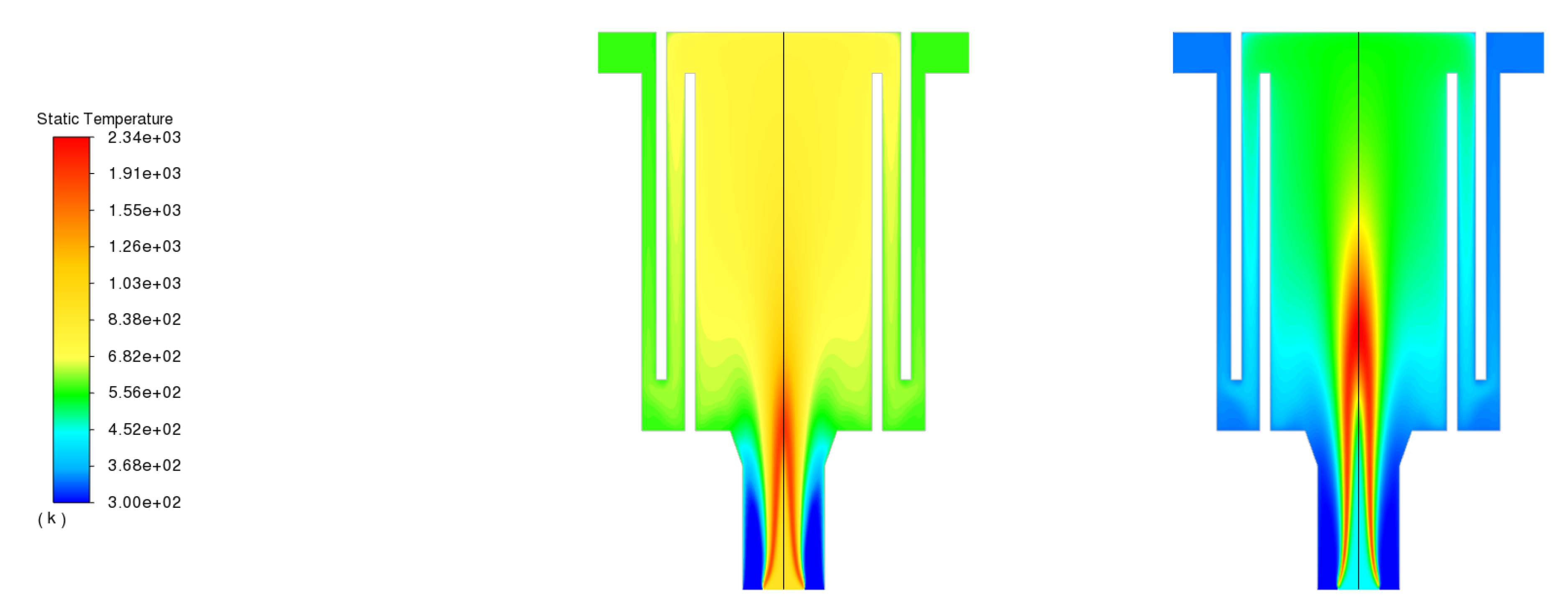
Figure 6 show the simulation results of the combustion of the lower and higher calorific gas mixtures obtained through the incorporated mechanism involving 77 reactions of H 2 and CO 
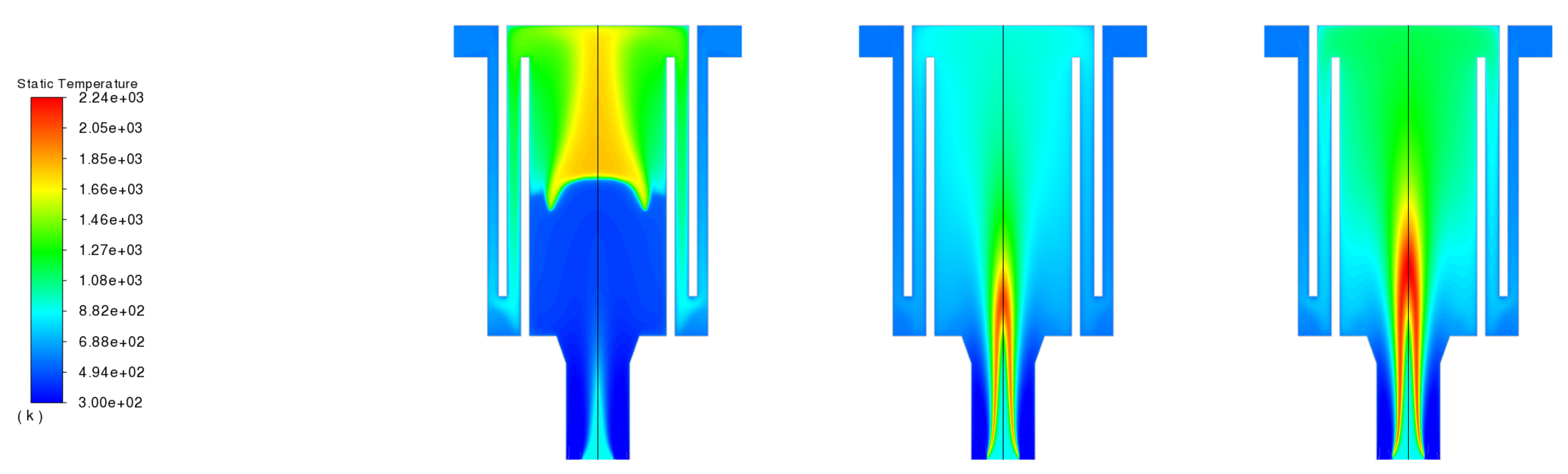
oxidation. As may be seen, the predicted temperature distributions in the boiler differ depending on the combusted volatile composition. Namely, for the lean gas mixture (with a heating value of approx. 6 MJ/kg), the burning area (the central flame) is shifted downwards, towards the inlet to the combustion chamber (Figure 3—left picture) as compared to the rich gas mixture combustion (of approx. 16 MJ/kg, Figure 3—right picture). The pyrolysis gas composition also translates into the maximum gas temperature which, as expected, is lower in the case of burning lower calorific value gas compared to the case of higher calorific value gas, i.e., 1920 K and 2340 K, respectively.
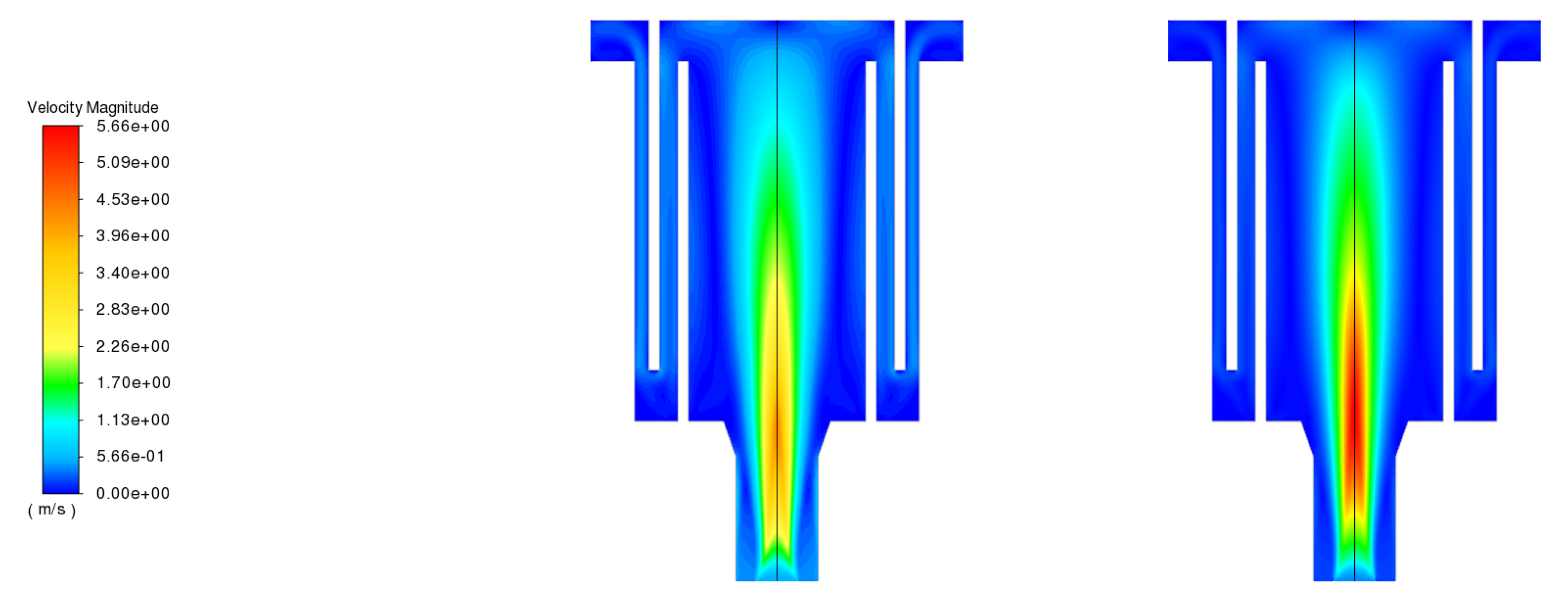
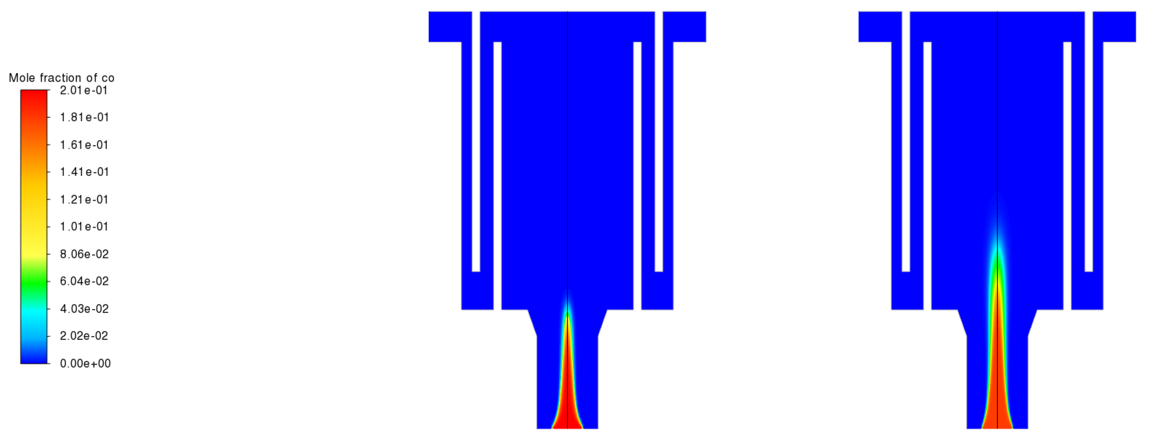
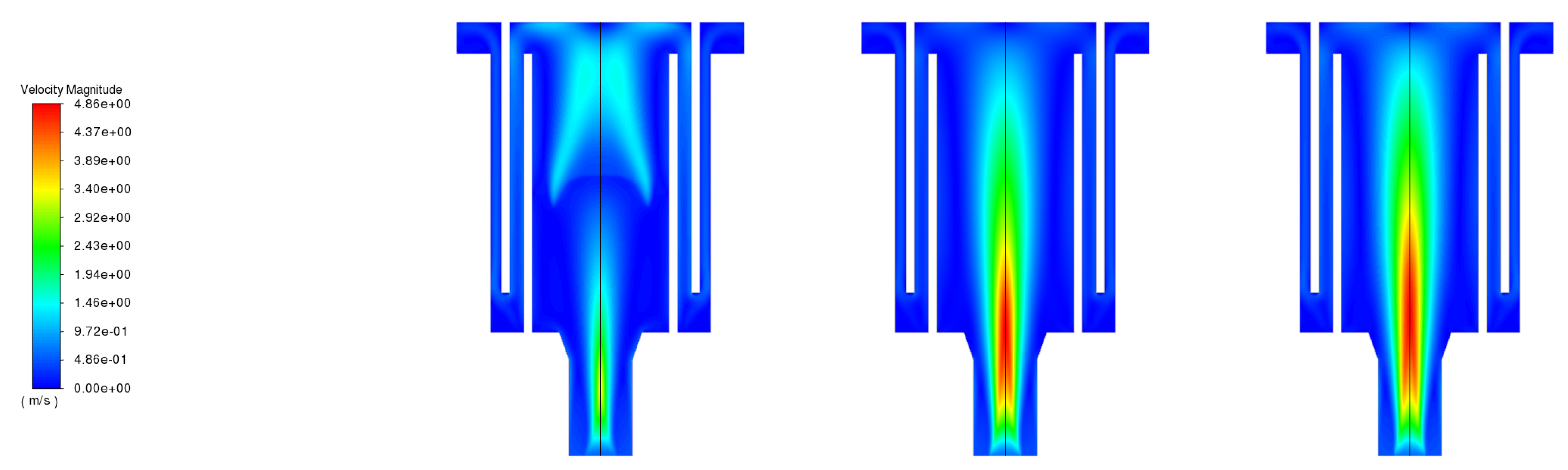
Moreover, the quality of gas affects the combustion process intensity, as illustrated by the gas velocity distribution (Figure 4). It is clearly seen from the simulation results that burning a rich gas mixture leads to higher gas velocities in the combustion zone. The difference in the process dynamics for various mixture compositions may be observed in Figure 5. The zone of oxidation in the gas mixture rich in CO (
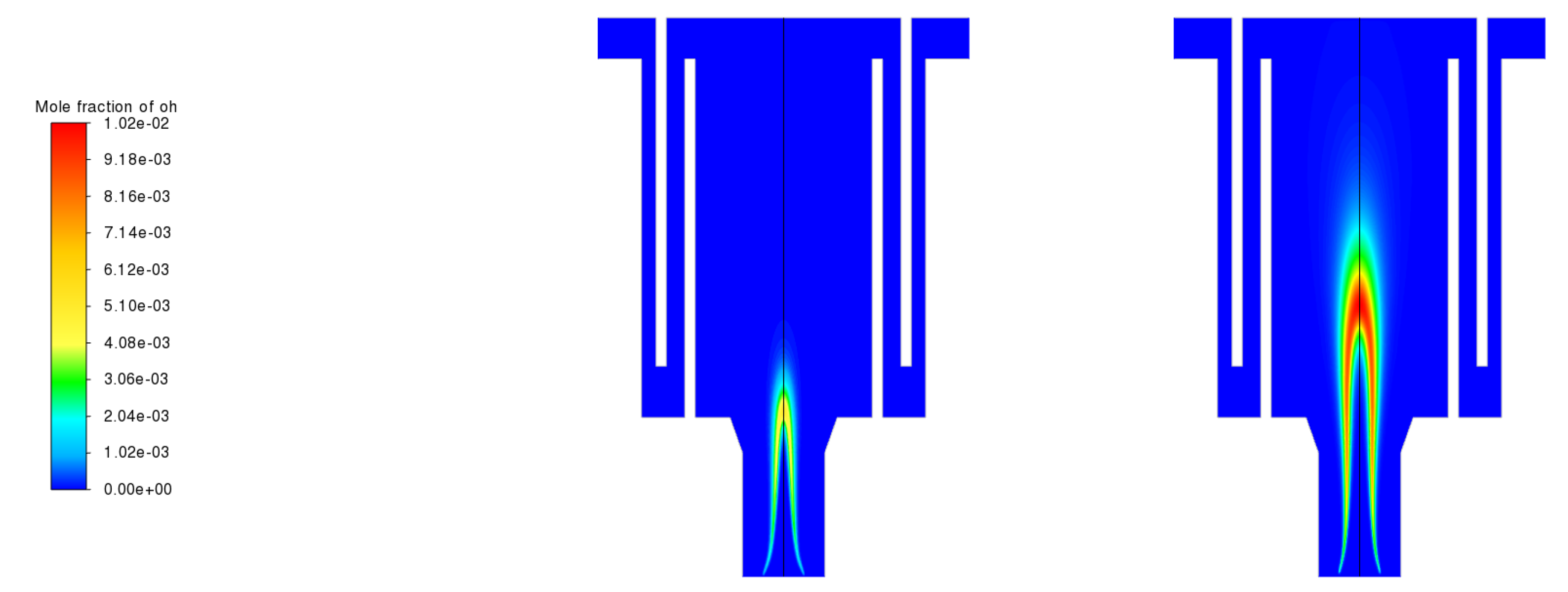
Figure 5 right picture) is extended, which results also from the velocity distribution of the gas stream. Furthermore, the flame spread in this case is nearly double that for the lower calorific value gas combustion, which is demonstrated by the distributions of hydroxyl radicals (OH) in the boiler chamber (Figure 6).
It may be observed that the combustion model applied in the analysis is promising in terms of predicting the oxidation characteristics of the H 2 / CO mixtures. It may however appear not sufficient when an additional reactant in the form of CH 4 is to be involved in the process. This may be evidenced by a too-high combustion temperature that was obtained in the simulation for the substitutive gas composition assumed, i.e., with increased fractions of CO and H 2 (Figure 3, Figure 4, Figure 5 and Figure 6, right).

3.2. RS85 Combustion Model of CH 4 / H 2 / CO

Figure 7, Figure 8, Figure 9, Figure 10, Figure 11 and Figure 12 present the results of a numerical analysis of the combustion of pyrolysis gas from various types of biomass: wood pellets, wood chips, and pine cones. The respective compositions of the released volatiles are provided in Table 4. For the record, the fractions of the combustible compounds (CH4/CO/H2) in pyrolysis gas mixtures determined for these fuels were predicted at 25%/8%/1%, 20%/7%/20%, and 25%/50%/41%, respectively.
The temperature distribution during the combustion of the given gas mixtures is presented in Figure 7. It is seen from the figure that the gas-burning zone for wood pellets has notably shifted toward the heat exchange section, unlike the two other cases under consideration (i.e., for wood chips and pine cones). Furthermore, the temperature of the pellets’ volatile combustion is about 300 K lower, even though this gas mixture has the highest calorific value amongst all mixtures analyzed. Moreover, it contains less than half of H 2 than the other mixtures considered in the study (see Table 4). Such a burning behavior that demonstrates the flame detachment is unfavorable in real operation conditions, in which the flame stability and its location in relation to the burner outlet are of concern. Hydrogen contents in the gas mixtures from wood chips and pine cones are similar; therefore, the simulations for these cases have resulted in similar temperature distributions in the boiler (Figure 7, middle and right). The location of the flame in the near-burner zone, which is predicted for these cases, translates to a more extensive high-temperature zone in the boiler core, thereby contributing to better heat exchange conditions. This also fosters enhanced heat transfer in a layer of devolatilized biomass particles and their ignition, resulting in a higher burner efficiency. Simultaneously, volatiles from pine cones are more calorific, which is reflected in the larger extent of the combustion zone that reaches the upper part of the heat exchange section as compared to the wood chips burning.
Combustion characteristics are reflected in the gas velocity field. The maximum velocities are identified just in the temperature front, and similar flow fields may be observed for gas mixtures of similar hydrogen percentages. The model predictions point to a more dynamic process in the case of the gas from chips and cones compared to wood pellet gas combustion (the maximum velocities amount to 4.8 m/s and 3.5 m/s, respectively), as shown in Figure 8.
Figure 9 illustrates the distribution of the CO mole fraction during the combustion of considered pyrolysis gas mixtures. It is seen that in each case, the highest CO concentrations are expected near the inlet to the boiler chamber, whereas when wood pellets are to be considered, the CO concentrations are completely oxidized in the upper half of a chamber (Figure 9, left). Simulation results for the combustion of wood chips and pine cones demonstrate the absence of this compound in the heat exchange section (Figure 9, middle and right pictures).
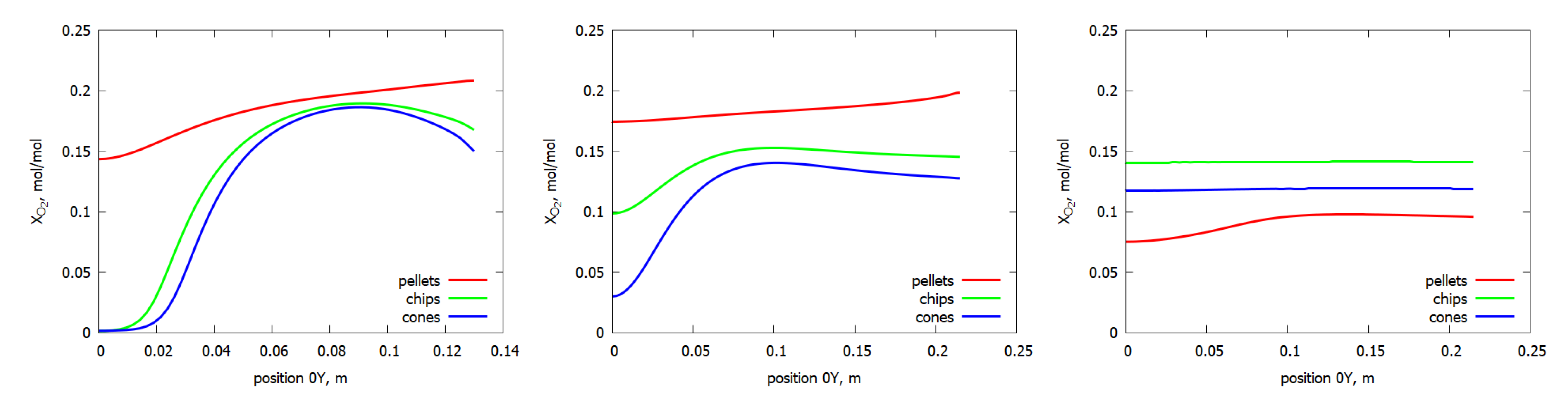
The combustion zone is also identified through the analysis of oxidizing reactants, as shown in Figure 10 and Figure 11. The first one displays the H 2 O concentration distribution, and the other presents the same for O 2 . It may be observed that the concentration of H 2 O increases where the O 2 concentration decreases. Furthermore, hydrogen oxidation takes place there. For the wood pellet case, there can be a prominent separation front between the zones of higher (below ∼21%) and lower (up to ∼14%) O 2 concentrations observed halfway up the inner coil. In the case of burning volatiles from wood chips and pine cones, most of the O 2 
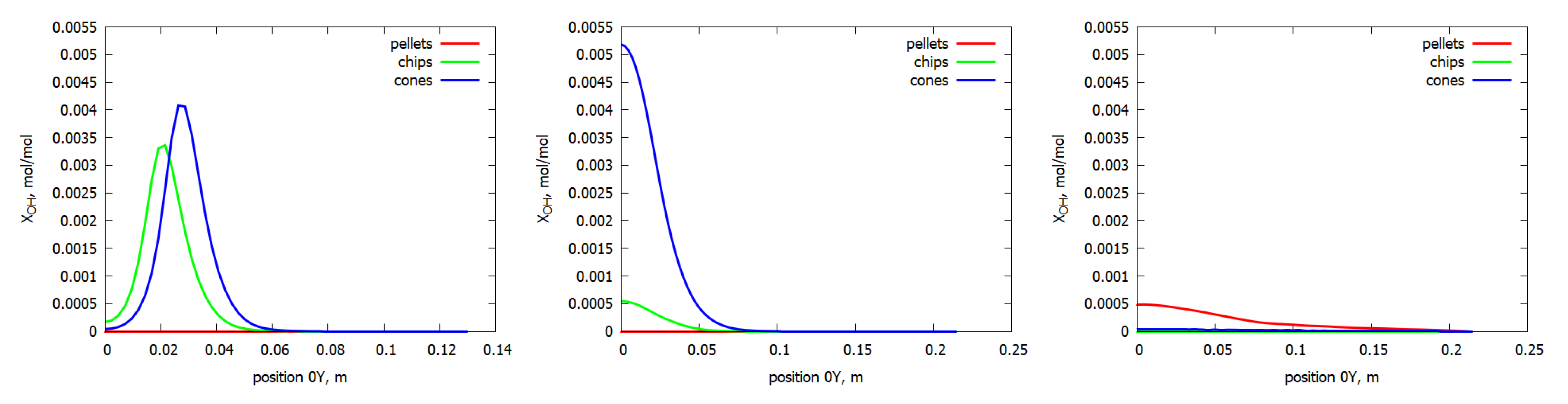
is consumed in the near-burner zone, and its distribution remains nearly constant along the boiler height above this zone. Again, the similarity in combustion behavior between volatiles released from wood chips and pine cones is noticeable. The flame zones are illustrated by the distribution of the hydroxyl radical (OH) mole fraction in Figure 12. In the case of wood pellets, the gases are combusted in the upper part of the inner coil, whereas in the case of the other fuels in the study, the process takes place at the inlet zone of the heat exchange section.
The qualitative comparison of the obtained results is summarized in Figure 13, Figure 14, Figure 15, Figure 16, Figure 17 and 
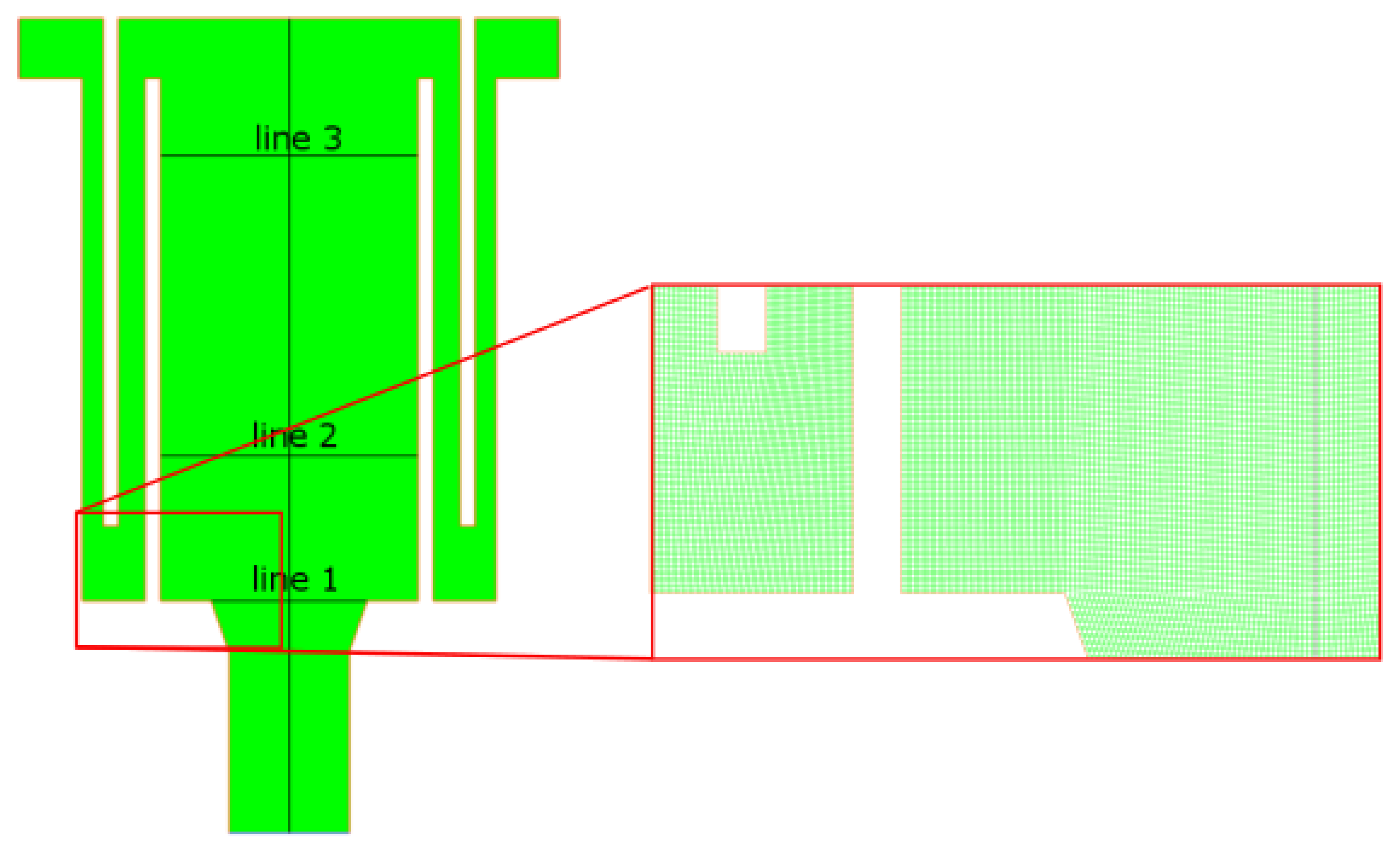
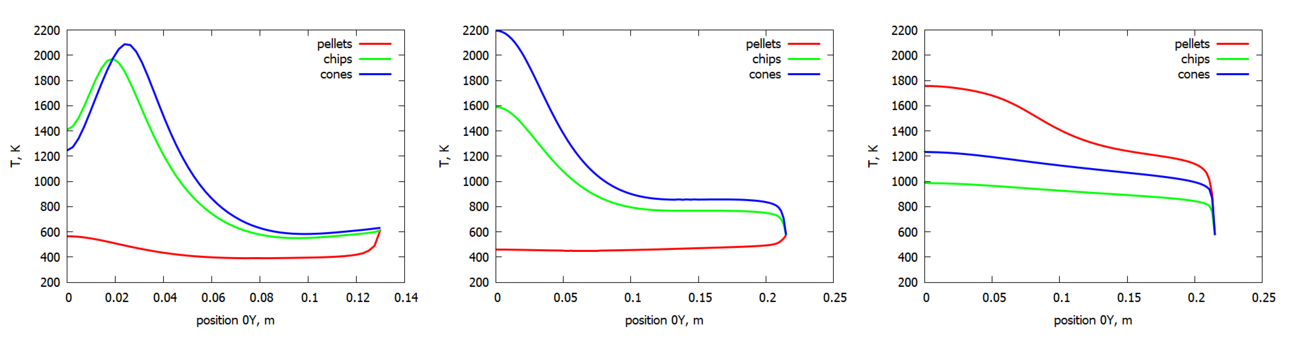
Figure 18. Each figure shows the given parameter change as a function of distance from the center line of a channel, i.e., from the center of the boiler core. In the figures, the red lines represent the respective parameters for the wood pellets, the green ones for the wood chips, and the blue lines refer to the pine cones. Each figure displays the parameters’ variation at three different boiler heights, as specified in Figure 2: line 1 indicates the inlet into the chamber, whereas lines 2 and 3 represent the distances of 242 mm and 742 mm above the inlet, respectively.
Based on the analysis of the temperature distribution for the respective fuels under study (Figure 13), it may be concluded that the gas combustion zone for the wood pellets is located closer to the upper part of the boiler, which is consistent with the contour map shown in Figure 7 (left picture). The predictions for the pyrolysis gas from the wood chips and pine cones indicate that the combustion zone is located rather closer to the inlet into the chamber, which also agrees with the temperature maps for those fuels (see Figure 7, middle, and right pictures, respectively). In addition, temperature distributions in line 3 show an average gas temperature of about 1000 K for the chips and pines, and of about 1500 K for the pellets. From the measurement data reported in [30], it follows that the temperature in the space between the inner and outer coils varied within the range of 670–730 K, which corresponded to the biomass burner power range of 19–26 kW. The average flue gas temperature in a similar location obtained from the simulation are ∼1000 K for pellets, ∼800 K for chips, and ∼900 K for cones (see Figure 7). For wood chips burning, the difference between the measured and predicted values does not exceed 10%. This suggests that the pyrolysis gas with higher contents of H 2 , as it is in the case for gas mixtures from wood chips and pine cones, better reflects the performance of a real unit. Following this thought, it may be concluded that under real operation conditions, pyrolysis gas combustion takes place rather at the near-inlet zone. Most of the heat transfer between the flue gas and the cooling oil takes place in the zone between the coils.
The graphs remaining in the figures demonstrate that the combustion behavior of the pyrolysis gas from the wood chips and pine cones is similar. Therefore, it may suggest that the composition of wood pellet volatiles might be underestimated.
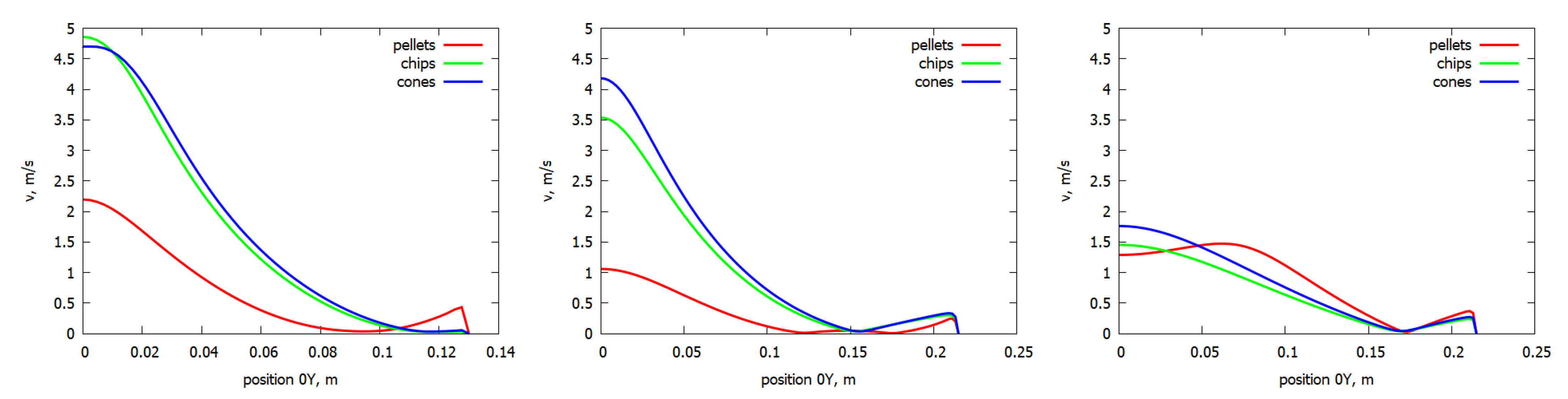
The velocity profiles presented in Figure 14 show that gases accelerate in the channel core, which is in agreement with the flow principles in the channels.
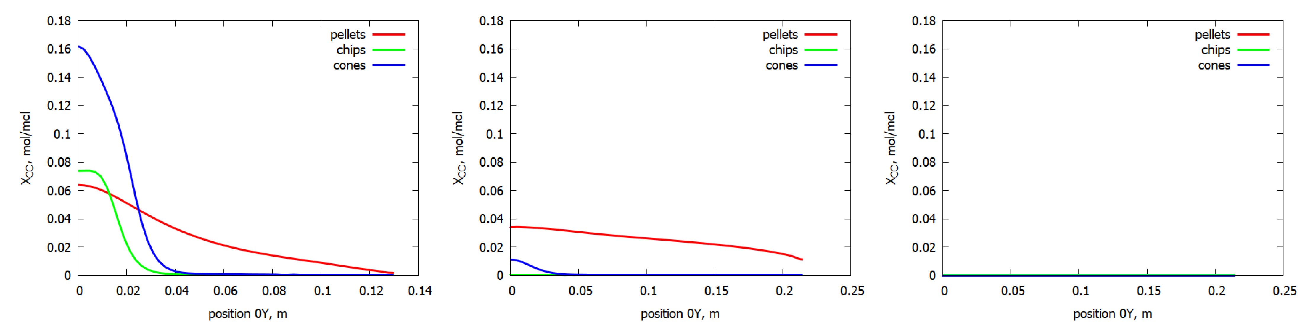
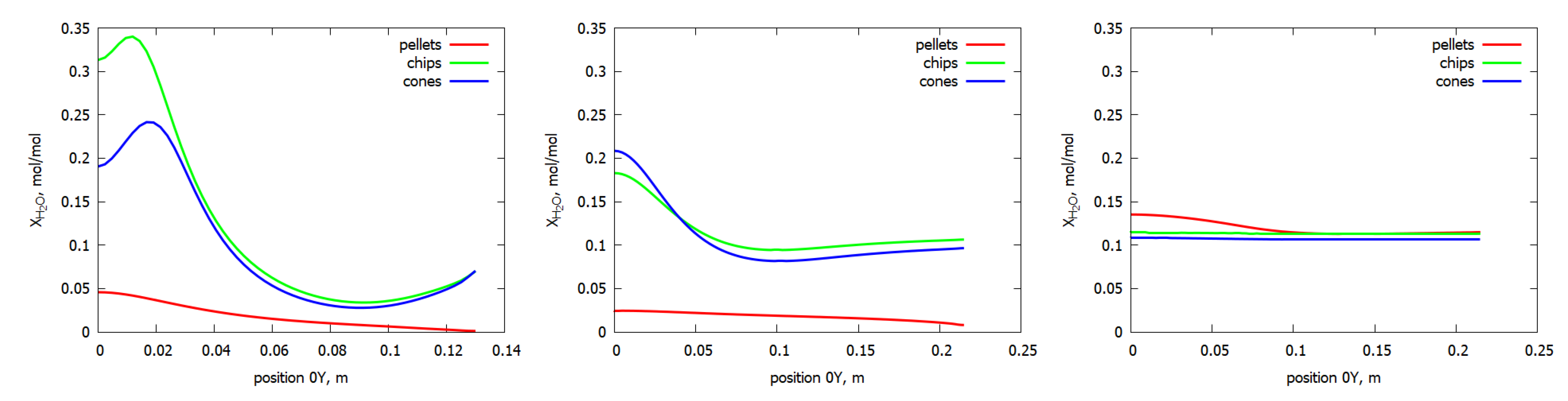
The burning zone characteristics for various fuels may be compared based on the concentration of particular chemical species. The mole fraction of CO decreases with the increase in the distance from the inlet for wood chips and pine cones. For wood pellets, it grows first and then it drops down (see Figure 15). This is also the case for H 2 O (Figure 16). For the pellets, the vapor concentration slightly diminishes at first, and increases afterward in the upper part of the inner coil core. Hence, it may be stated that the combustion zone for wood pellet volatiles is shifted towards the upper section of the boiler, whereas for other considered fuels, it remains in the inlet channel of the heat exchange part. The generation of H 2 O is related to oxygen consumption, according to the global reaction of hydrocarbon oxidation, as can be seen in the graphs depicted in Figure 17. The trend in the O 2 concentration change is the opposite. Namely, for pellets, it initially slightly grows and subsequently diminishes with the increased distance from the inlet to the core of the inner coil. For the other fuels, the O 2 concentration increases along with the boiler height.
The location of the burning front is well demonstrated by the OH radicals’ concentration level. Numerical results displayed in Figure 18 indicate that in the case of the wood chips and pine cones, the flame is located in the inlet channel of the boiler heat exchange section, and in the case of the wood pellet combustion (line 3), it is expected to be shifted to the upper part of the boiler.

4. Summary

The paper presents the results of a numerical analysis of pyrolysis gas combustion generated from biomass in a small-scale coil-type boiler. For this purpose, the numerical simulations were carried out, taking into account various detailed mechanisms of pyrolysis gas combustion. These involved the implementation of two chemical kinetics models, one with 77 elemental reactions (RS77) describing the oxidation of CO / H 2 mixtures, and the second with 85 reactions (RS85) for the combustion of the CH 4 / CO / H 2 mixtures. The initial gas compositions were determined utilizing the equilibrium-based approach, involving the Gibbs function minimization method. The geometry of the system has been simplified into a 2D model, covering the whole area of flue gas circulation. The analysis helped to recognize some general features of volatile burning for three different biomass fuels, thereby contributing to the challenging task of predicting their combustion characteristics. The main outcomes derived from the study may be summarized as follows:
(1) As far as the combustion of pyrolysis gas is to be considered, the 2D model coupling thermodynamic equilibrium with chemical kinetics provides reliable predictions of biomass combustion characteristics. At the same time, the enhanced chemical kinetics model (RS85) was found to be more reliable than the RS77 model, particularly for the relatively high content of methane;
(2) Still, the cost-effectiveness of the process simulation in terms of computation time shall always be of concern. The RS85 mechanism, despite that it is more advanced, appeared to offer a reasonable time in the case of the 2D case simulations. The applied approach might therefore be successfully used in 3D calculations for detailed boiler geometry if only the computation time would not be an issue of high priority;
(3) The gas-burning zone for wood pellets is notably shifted towards the heat exchange section. For wood chips and pine cones, the flame is predicted to be located in the near-burner zone, which translates to a more extensive high-temperature zone in the boiler core and contributes to better heat exchange conditions; and
(4) The comparison of the numerical results and experimental study data of a small-scale boiler showed that the predictions for volatiles containing less CH 4 and more H 2 comply with the combustion behavior under real operation conditions of the boiler.

Author Contributions

Conceptualization, D.K.; methodology, I.W.-Ś. and S.P.-K.; software, I.W.-Ś.; validation, I.W.-Ś. and S.P.-K.; formal analysis, I.W.-Ś. and S.P.-K.; investigation, I.W.-Ś. and S.P.-K.; writing—original draft preparation, I.W.-Ś. and S.P.-K.; writing—review and editing, D.K., I.W.-Ś. and S.P.-K.; visualization, I.W.-Ś. All authors have read and agreed to the published version of the manuscript.

Funding

This research received no external funding.

Institutional Review Board Statement

Not applicable.

Acknowledgments

This research was supported by computer centre CI TASK.

Conflicts of Interest

The authors declare no conflict of interest.

Abbreviations

The following abbreviations are used in this manuscript:
CFD  Computational Fluid Dynamics
DEM  Discrete Element Method
DPM  Discrete Phase Model
TGA  Thermogravimetric Analysis

References

  1. Roni, M.S.; Chowdhury, S.; Mamun, S.; Marufuzzaman, M.; Lein, W.; Johnson, S. Biomass co-firing technology with policies, challenges, and opportunities: A global review. Renew. Sustain. Energy Rev. 2017, 78, 1089–1101. [Google Scholar] [CrossRef]
  2. Zarzycki, R.; Kobyłecki, R.; Bis, Z. Numerical Analysis of the Combustion of Gases Generated during Biomass Carbonization. Entropy 2020, 22, 181. [Google Scholar] [CrossRef] [Green Version]
  3. International Energy Agency (IEA). Net Zero by 2050, A Roadmap for the Global Energy Sector. 2021. Available online: https://iea.blob.core.windows.net/assets/deebef5d-0c34-4539-9d0c-10b13d840027/NetZeroby2050-ARoadmapfortheGlobalEnergySector_CORR.pdf (accessed on 14 February 2021).
  4. Niemelä, C.P.; Mylläri, F.; Kuittinen, N.; Aurela, M.; Helin, A.; Kuula, J.; Teinilä, K.; Nikka, M.; Vainio, O.; Arffman, A.; et al. Experimental and numerical analysis of fine particle and soot formation in a modern 100 MW pulverized biomass heating plant. Combust. Flame 2022, 240, 111960. [Google Scholar] [CrossRef]
  5. Tu, Y.; Zhou, A.; Xu, M.; Yang, W.; Siah, K.B.; Subbaiah, P. NOx reduction in a 40 t/h biomass fired grate boiler using internal flue gas recirculation technology. Appl. Energy 2018, 220, 962–973. [Google Scholar] [CrossRef]
  6. Zadravec, T.; Yin, C.; Kokalj, F.; Samec, N.; Rajh, B. The impacts of different profiles of the grate inlet conditions on freeboard CFD in a waste wood-fired grate boiler. Appl. Energy 2020, 268, 115055. [Google Scholar] [CrossRef]
  7. Collazo, J.; Porteiro, J.; Míguez, J.L.; Granada, E.; Gómez, M.A. Numerical simulation of a small-scale biomass boiler. Energy Convers. Manag. 2012, 64, 87–96. [Google Scholar] [CrossRef]
  8. Aarchan, G.; Anca-Couce, A.; Buchmayr, M.; Hochenauer, C.; Gruber, J.; Scharler, R. Experimental evaluation of primary measures for NOx and dust emission reduction in a novel 200 kW multi-fuel biomass boiler. Renew. Energy 2021, 170, 1186–1196. [Google Scholar] [CrossRef]
  9. Feldmeier, S.; Schwarz, M.; Wopienka, E.; Pfeifer, C. Categorization of small-scale biomass combustion appliances by characteristic numbers. Renew. Energy 2021, 163, 2128–2136. [Google Scholar] [CrossRef]
  10. Hupa, M.; Karlström, O.; Vainio, E. Biomass combustion technology development—It is all about chemical details. Proc. Combust. Inst. 2016, 36, 113–134. [Google Scholar] [CrossRef]
  11. Kantorek, M.; Jesionek, K.; Polesek-Karczewska, S.; Ziółkowski, P.; Badur, J. Thermal utilization of meat and bone meals. Performance analysis in terms of drying process, pyrolysis and kinetics of volatiles combustion. Fuel 2019, 254, 115548. [Google Scholar] [CrossRef]
  12. Opydo, M.; Kobyłecki, R.; Dudek, A.; Bis, Z. The effect of biomass co-combustion in a CFB boiler on solids accumulation on surfaces of P91 steel tube samples. Biomass Bioenergy 2016, 85, 61–68. [Google Scholar] [CrossRef]
  13. Capablo, J.; Salvado, J. Estimating heat transfer losses caused by alkali salt deposits in biomass combustion. Renew. Energy 2017, 105, 449–457. [Google Scholar] [CrossRef]
  14. Kardaś, D.; Klonowicz, P.; Polesek-Karczewska, S.; Żywica, G. Technical aspects of small-scale biomass-fueled gas turbine power unit with a focus on high-temperature air furnace. In Proceedings of the 14th International Conference on Boiler Technology (ICBT), Szczyrk, Poland, 25–28 October 2022; Walewski, A., Gramatyka, F., Eds.; Politechnika Śląska: Gliwice, Poland, 2022. [Google Scholar]
  15. Pronobis, M. Evaluation of the influence of biomass co-combustion on boiler furnace slagging by means of fusibility correlations. Biomass Bioenergy 2005, 28, 375–383. [Google Scholar] [CrossRef]
  16. Capablo, J. Formation of alkali salt deposits in biomass combustion. Fuel Process Technol. 2016, 153, 58–73. [Google Scholar] [CrossRef]
  17. Chapela, S.; Cid, N.; Porteiro, J.; Míguez, J.L. Numerical transient modelling of the fouling phenomena and its influence on thermal performance in a low-scale biomass shell boiler. Renew. Energy 2020, 161, 309–318. [Google Scholar] [CrossRef]
  18. Obernberger, I.; Brunner, T.; Mandl, C.; Kerschbaum, M.; Svetlik, T. Strategies and technologies towards zero emission biomass combustion by primary measures. Energy Procedia 2017, 120, 681–688. [Google Scholar] [CrossRef]
  19. Anca-Couce, A.; Hochenauer, C.; Scharler, R. Bioenergy technologies, uses, market and future trends with Austria as a case study. Renew. Sustain. Energy Rev. 2021, 135, 110237. [Google Scholar] [CrossRef]
  20. Polesek-Karczewska, S.; Turzyński, T.; Kardaś, D.; Heda, Ł. Front velocity in the combustion of blends of poultry litter with straw. Fuel Proc. Technol. 2018, 176, 307–315. [Google Scholar] [CrossRef]
  21. Turzyński, T.; Kluska, J.; Ochnio, M.; Kardaś, D. Comparative Analysis of Pelletized and Unpelletized Sunflower Husks Combustion Process in a Batch-Type Reactor. Materials 2021, 14, 2484. [Google Scholar] [CrossRef] [PubMed]
  22. Gómez, M.A.; Martín, R.; Chapela, S.; Porteiro, J. Steady CFD combustion modeling for biomass boilers: An application to the study of the exhaust gas recirculation performance. Energy Convers. Manag. 2019, 179, 91–103. [Google Scholar] [CrossRef]
  23. Tabet, F.; Gökalp, I. Review on CFD based models for co-firing coal and biomass. Renew. Sustain. Energy Rev. 2015, 51, 1101–1114. [Google Scholar] [CrossRef]
  24. Peters,, B.; Baniasadi, M.; Baniasadi, M.; Besseron,, X.; Estupinan Donoso, A.; Mohseni, M.; Pozzetti,, G. XDEM multi-physics and multi-scale simulation technology: Review of DEM–CFD coupling, methodology and engineering applications. Particuology 2019, 44, 176–193. [Google Scholar]
  25. Marangwanda, G.T.; Madyira, D.M.; Babarinde, T.O. Combustion models for biomass: A review. Energy Rep. 2020, 6, 664–672. [Google Scholar]
  26. Mehrabian, R.; Shiehnejadhesar, A.; Scharler, R.; Obernberger, I. Multi-physics modelling of packed bed biomass combustion. Fuel 2014, 122, 164–178. [Google Scholar] [CrossRef]
  27. Villermaux, J.; Antoine, B.; Lede, J.; Soulignac, F. A new model for thermal volatilization of solid particles undergoing fast pyrolysis. Chem. Eng. Sci. 1986, 41, 151–157. [Google Scholar] [CrossRef]
  28. Bellais, M.; Davidsson, K.; Liliedahl, T.; Sjöström, K.; Pettersson, J. Pyrolysis of large wood particles: A study of shrinkage importance in simulations? Fuel 2003, 82, 1541–1547. [Google Scholar] [CrossRef]
  29. Popescu, F.; Mahu, R.; Ion, I.V.; Rusu, E. A Mathematical Model of Biomass Combustion Physical and Chemical Processes. Energies 2020, 13, 6232. [Google Scholar] [CrossRef]
  30. Polesek-Karczewska, S.; Wardach-Święcicka, I.; Kardaś, D.; Turzyński, T. Application of a Lumped Multi-Section Model for Analyzing the Thermal Performance of a Small-Scale Biomass Boiler. J. Therm. Sci. 2021, 30, 1034–1045. [Google Scholar] [CrossRef]
  31. Aria, H.; Akhavan-Behabadi, M.A.; Shemirani, F.M. Experimental investigation on flow boiling heat transfer and pressure drop of HFC-134a inside a vertical helically coiled tube. Heat Transf. Eng. 2012, 33, 79–87. [Google Scholar] [CrossRef]
  32. Beigzadeh, R.; Rahimi, M.; Parvizi, M. Experimental study and genetic algorithm-based multi-objective optimization of thermal and flow characteristics in helically coiled tubes. Heat Mass Transf 2013, 49, 1307–1318. [Google Scholar] [CrossRef]
  33. Gomma, A.; Aly, W.I.A.; Omara, M.; Abdelmagied, M. Correlations for heat transfer coefficient and pressure drop in the annulus of concentric helical coils. Heat Mass Transf 2014, 50, 583–586. [Google Scholar] [CrossRef]
  34. Patil, R.H. Isothermal laminar fluid flow in spiral tube coils. Heat Mass Transf 2018, 54, 3673–3693. [Google Scholar] [CrossRef]
  35. ANSYS FLUENT 12.0 Theory Guide ANSYS, Inc. 2009. Release 12.0. Available online: https://www.afs.enea.it/project/neptunius/docs/fluent/html/th/main_pre.htm (accessed on 7 April 2023).
  36. Wardach-Święcicka, I.; Kardaś, D. Prediction of Pyrolysis Gas Composition Based on the Gibbs Equation and TGA Analysis. Energies 2023, 16, 1147. [Google Scholar] [CrossRef]
  37. Phan, A.N.; Ryu, C.; Sharifi, V.N.; Swithenbank, J. Characterisation of slow pyrolysis products from segregated wastes for energy production. J. Anal. Appl. Pyrolysis 2008, 81, 65–71. [Google Scholar] [CrossRef]
  38. Senneca, O. Kinetics of pyrolysis, combustion and gasification of three biomass fuels. Fuel Process Technol. 2007, 88, 87–97. [Google Scholar] [CrossRef]
  39. Bielański, A. General and Inorganic Chemistry; John Wiley & Sons: Warsaw, Poland, 1970. (In Polish) [Google Scholar]
  40. Starik, A.M.; Titova, N.S.; Sharipov, A.S.; Kozlov, V.E. Syngas Oxidation Mechanism. Combust. Explos Shock Waves 2010, 40, 491–506. [Google Scholar] [CrossRef]
  41. Kee, R.J.; Rupley, F.M.; Meeks, E.; Miller, J. CHEMKIN–III: Fortran Chemical Kinetics Package for the Analysis of Gas–Phase Chemical and Plasma Kinetics; Sandria National Laboratories: Livermore, CA, USA, 1996. [Google Scholar]
  42. Fuel Gases-Heating Values. Available online: https://www.engineeringtoolbox.com/heating-values-fuel-gases-d_823.html (accessed on 14 February 2019).
  43. Kazakov, A.; Frenklach, M. Reduced Version of GRI-MECH 1.2, 22 Species. 1994. Available online: http://www.me.berkeley.edu/drm/ (accessed on 14 February 2019).
  44. Smith, G.P.; Golden, D.M.; Frenklach, M.; Moriarty, N.W.; Eiteneer, B.; Goldenberg, M.; Bowman, C.T.; Hanson, R.K.; Song, S.; Gardiner, W.C., Jr.; et al. 1999. Available online: http://www.me.berkeley.edu/gri_mech/ (accessed on 14 February 2019).
Figure 1. Experimental set up for oil-cooled coiled tube boiler fired with biomass, IMP PAN [30].
Applmech 04 00040 g001
Figure 2. Computational domain.
Applmech 04 00040 g002
Figure 3. Temperature distribution (K): lower (left) and higher calorific value gas (right).
Applmech 04 00040 g003
Figure 4. Velocity magnitude distribution (m/s): lower (left) and higher calorific value gas (right).
Applmech 04 00040 g004
Figure 5. CO mole fraction (kmol/kmol): lower (left) and higher calorific value gas (right).
Applmech 04 00040 g005
Figure 6. OH mole fraction (kmol/kmol): lower (left) and higher calorific value gas (right).
Applmech 04 00040 g006
Figure 7. Temperature distribution (K): wood pellets (left), wood chips (middle), and pine cones (right).
Applmech 04 00040 g007
Figure 8. Velocity distribution (m/s): wood pellets (left), wood chips (middle), and pine cones (right).
Applmech 04 00040 g008
Figure 9. Mole fraction of CO (mol/mol): wood pellets (left), wood chips (middle), and pine cones (right).
Applmech 04 00040 g009
Figure 10. Mole fraction of H 2 O (mol/mol): wood pellets (left), wood chips (middle), and pine cones (right).
Applmech 04 00040 g010
Figure 11. Mole fraction of O 2 (mol/mol): wood pellets (left), wood chips (middle), and pine cones (right).
Applmech 04 00040 g011
Figure 12. Mole fraction of OH (mol/mol): wood pellets (left), wood chips (middle), and pine cones (right).
Applmech 04 00040 g012
Figure 13. Temperature distribution (K): line 1 (left), line 2 (middle), and line 3 (right).
Applmech 04 00040 g013
Figure 14. Velocity distribution (m/s): line 1 (left), line 2 (middle), and line 3 (right).
Applmech 04 00040 g014
Figure 15. Mole fraction of CO (mol/mol): line 1 (left), line 2 (middle), and line 3 (right).
Applmech 04 00040 g015
Figure 16. Mole fraction of H 2 O (mol/mol): line 1 (left), line 2 (middle), and line 3 (right).
Applmech 04 00040 g016
Figure 17. Mole fraction of O 2 (mol/mol): line 1 (left), line 2 (middle), and line 3 (right).
Applmech 04 00040 g017
Figure 18. Mole fraction of OH (mol/mol): line 1 (left), line 2 (middle), and line 3 (right).
Applmech 04 00040 g018
Table 1. Technical and elemental analyses of wood pellets [37].
Technical Analysis %
StateAs receivedDryDry ash free
Volatiles71.7077.0279.49
Fixed carbon18.5019.8720.51
Moisture6.90--
Ash2.903.11-
Elemental Analysis %
StateAs receivedDryDry ash free
C44.9048.2349.78
H7.467.207.43
O44.7441.4642.79
Ash2.903.11-
Table 2. Technical and elemental analyses of wood chips [38].
Technical Analysis %
StateAs receivedDryDry ash free
Volatiles51.6079.2079.52
Fixed carbon13.3020.4020.48
Moisture34.90--
Ash0.200.40-
Elemental Analysis %
StateAs receivedDryDry ash free
C30.7947.3047.49
H7.856.106.12
O61.0346.0046.19
N0.130.200.20
Ash0.200.40-
Table 3. Technical and elemental analyses of pine cones [38].
Technical Analysis %
StateAs receivedDryDry ash free
Volatiles69.2077.3778.07
Fixed carbon19.4021.7321.93
Moisture10.30--
Ash1.100.90-
Elemental Analysis %
stateAs receivedDryDry ash free
C43.5048.5048.94
H6.626.106.16
O48.6044.3044.70
N0.180.200.20
Ash1.100.90-
Table 4. Pyrolysis gas composition for the considered fuels.
Wood PelletsWood ChipsPine Cones
T = 900 KX, mol/mol %Y, kg/kg %X, mol/mol %Y, kg/kg %X, mol/mol %Y, kg/kg %
CH 4 25.1120.570.940.928.297.57
CO 20.1528.816.5811.1919.8331.63
CO 2 15.4234.6521.1456.5016.3540.98
H 2 O 14.4413.2823.1925.3714.5214.80
H 2 24.782.5548.075.8840.874.69
N 2 0.100.140.080.140.140.23
H H V , MJ / kg 16.268.6515.52
Table 5. Boundary conditions.
AirVolatilesWall
m ˙ a i r , i n l e t = 0.0123 kg/s m ˙ g a s , i n l e t = 0.00123 kg/s-
T a i r , i n l e t = 300 K T g a s , i n l e t = 900 K T w a l l , c o i l s = 532 K
Table 6. List of the reactions adopted for the pyrolysis gas combustion model with the values of the Arrhenius equation constants [40].
No.ReactionA, ( cm 3 / mol ) n 1 / ( K n s ) n E a , cal/mol
Group I: reactions with the participation of O 2 , H 2 , O, H, H 2 O
1 H 2 O + H = OH + H 2 8.4 × 10130.0020,029.68
2 OH + H 2 = H 2 O + H 2.0 × 10130.005148.00
3 O 2 + H = OH + O 2.20 × 10140.0016,740.90
4 OH + O = O 2 + H 1.30 × 10130.00693.00
5 H 2 + O = OH + H 1.80 × 10101.008870.40
6 OH + H = H 2 + O 8.30 × 1091.006930.00
7 O 2 + M = 2 O + M 5.40 × 10¹⁸−1.00117,612.00
8 2 O + M = O 2 + M 6.00 × 10130.00−1782.00
9 H 2 + M = 2 H + M 2.20 × 10140.0095,634.00
10 2 H + M = H 2 + M 9.00 × 10¹⁷−1.000.00
11 H 2 O + M = OH + H + M 1.00 × 1024−2.20116,820.00
12 OH + H + M = H 2 O + M 2.20 × 10²²−2.000.00
13 OH + M = O + H + M 8.50 × 10¹⁸−1.00100,643.40
14 O + H + M = OH + M 7.10 × 10¹⁸−1.000.00
15 H 2 O + O = 2 OH 5.80 × 10130.0017,936.82
16 2 OH = H 2 O + O 5.30 × 10120.00995.94
Group II: reactions with the participation of HO 2
17 H + O 2 ( + M ) = HO 2 ( + M ) 3.50 × 10¹⁶−0.41−1118.70
18 H 2 + O 2 = H + HO 2 7.39 × 1052.4353,313.48
19 H 2 O + O = H + HO 2 4.76 × 10110.37256,911.14
20 H + HO 2 = H 2 O + O 1.00 × 10130.001069.20
21 H 2 O + O 2 = OH + HO 2 1.50 × 10150.5072,468.00
22 OH + HO 2 = H 2 O + O 2 3.00 × 10140.000.00
23 2 OH = H + HO 2 1.20 × 10130.0039,996.00
24 H + HO 2 = 2 OH 2.50 × 10140.001881.00
25 OH + O 2 = O + HO 2 1.30 × 10130.0055,836.00
26 O + HO 2 = OH + O 2 5.00 × 10130.003762.00
Group III: reactions with the participation of H 2 O 2
27 H + H 2 O 2 = H 2 + HO 2 1.7 × 10120.003762.00
28 H 2 + HO 2 = H + H 2 O 2 6.00 × 10110.0018,414.00
29 H + H 2 O 2 = H 2 O + OH 5.00 × 10140.009900.00
30 H 2 O + OH = H + H 2 O 2 2.40 × 10140.0080,190.00
31 2 HO 2 = H 2 O 2 + O 2 1.80 × 10130.00990.00
32 H 2 O 2 + O 2 = 2 HO 2 3.00 × 10130.0042,786.00
33 HO 2 + H 2 O = H 2 O 2 + OH 1.80 × 10130.0029,898.00
34 H 2 O 2 + OH = HO 2 + H 2 O 1.00 × 10130.001801.80
35 OH + HO 2 = H 2 O 2 + O 5.20 × 10100.5020,988.00
36 H 2 O 2 + O = OH + HO 2 2.00 × 10130.005860.80
37 H 2 O 2 + M = 2 OH + M 1.20 × 10170.0045,342.00
38 2 OH + M = H 2 O 2 + M 9.10 × 10140.00−5247.00
Group IV: reactions with the participation of O 3
39 O 3 + M = O 2 + O + M 4.00 × 10140.0022,572.00
40 O 2 + O + M = O 3 + M 6.90 × 10120.00−2079.00
41 O 3 + H = OH + O 2 2.30 × 10110.750.00
42 OH + O 2 = O 3 + H 4.40 × 1071.4476,428.00
43 O 3 + O = 2 O 2 1.10 × 10130.004554.00
44 2 O 2 = O 3 + O 1.20 × 10130.0099,990.00
45 O 3 + OH = HO 2 + O 2 9.6 × 10110.001980.00
46 O 3 + H 2 = OH + HO 2 6.02 × 10100.0019,800.00
47 O 3 + HO 2 = OH + 2 O 2 2.00 × 10100.001980.00
Group V: reactions with the participation of CO
48 CO + O 2 = CO 2 + O 3.20 × 10110.0037,521.00
49 CO 2 + O = CO + O 2 2.80 × 10120.0043,738.20
50 CO + O ( + M ) = CO 2 ( + M ) 1.55 × 1024−2.794193.64
51 CO + OH = CO 2 + H 1.51 × 1071.30−768.438
52 CO 2 + H = CO + OH 1.70 × 1091.3021,535.074
53 CO + HO 2 = CO 2 + OH 1.15 × 1052.2817,521.02
Group VI: reactions with the participation of HCO
54 HCO + M = H + CO + M 4.75 × 10110.7014,875.74
H 2 / 2.5 / H 2 O / 6 / CO / 1.9 / CO 2 / 3.8 /
55 HCO + H 2 = CH 2 O + H 2.63 × 10130.0025,118.28
56 CH 2 O + H = HCO + H 2 5.01 × 10130.003991.68
57 CO + HO 2 = HCO + O 2 8.91 × 10120.0032,222.52
58 HCO + O 2 = CO + HO 2 3.02 × 10120.000.00
59 CO + H 2 = HCO + H 1.32 × 10150.0089,812.80
60 HCO + H = CO + H 2 1.2 × 10140.000.00
61 HCO + O = H + CO 2 3.01 × 10130.000.00
62 HCO + O = OH + CO 1.00 × 10140.000.00
63 OH + CO = HCO + O 2.88 × 101440.0087,717.96
64 HCO + OH = H 2 O + CO 3.16 × 10130.000.00
65 H 2 O + CO = HCO + OH 8.91 × 101440.00104,880.60
66 2 HCO = H 2 + 2 CO 3.01 × 10120.000.00
Group VII: reactions with the participation of CH 2 O
67 2 HCO = CH 2 O + CO 1.81 × 10130.000.00
68 CH 2 O + M = H + HCO + M 3.31 × 101460.0080,831.52
69 H + HCO + M = CH 2 O + M 1.41 × 10110.00−11,775.06
70 CH 2 O + O 2 = HO 2 + HCO 3.63 × 10150.0045,943.92
71 HO 2 + HCO = CH 2 O + O 2 1.00 × 10140.002993.76
72 CH 2 O + O = HCO + OH 5.01 × 10130.004589.64
73 HCO + OH = CH 2 O + O 1.74 × 10120.0017,134.92
74 CH 2 O + OH = HCO + H 2 O 3.47 × 1091.20−479.16
75 HCO + H 2 O = CH 2 O + OH 1.17 × 1091.2029,307.96
76 CH 2 O + HO 2 = H 2 O 2 + HCO 2.00 × 10110.007983.36
77 H 2 O 2 + HCO = CH 2 O + HO 2 2.19 × 10140.006575.58
Table 7. Pyrolysis gas composition.
T = 900 KY, kg/kg %
Heating value, MJ/kg5.9816.27
CH 4 0.00.0
CO 28.8141.91
CO 2 34.6434.64
H 2 O 13.2813.28
H 2 2.5510.02
O 2 0.000.00
N 2 20.720.15
Table 8. List of the reactions of the reduced methane combustion model with the values of the Arrhenius equation constants [43].
No.ReactionA, ( cm 3 / mol ) n 1 / ( K n s ) n E a , cal/mol
R1 O + H + M < = > OH + M 5.000 × 10¹⁷−1.0000.00
H 2 / 2.00 / H 2 O / 6.00 / CH 4 / 2.00 / CO / 1.50 / CO 2 / 2.00 / C 2 H 6 / 3.00 / AR / 0.70 /
R2 O + H 2 < = > H + OH 5.000 × 1042.6706290.00
R3 O + HO 2 < = > OH + O 2 2.000 × 10130.0000.00
R4 O + CH 2 < = > H + HCO 8.000 × 10130.0000.00
R5 O + CH 2 ( S ) < = > H + HCO 1.500 × 10130.0000.00
R6 O + CH 3 < = > H + CH 2 O 8.430 × 10130.0000.00
R7 O + CH 4 < = > OH + CH 3 1.020 × 10091.5008600.00
R8 O + CO + M < = > CO 2 + M 6.020 × 10140.0003000.00
H 2 / 2.00 / O 2 / 6.00 / H 2 O / 6.00 / CH 4 / 2.00 / CO / 1.50 / CO 2 / 3.50 / C 2 H 6 / 3.00 / AR / 0.50 /
R9 O + HCO < = > OH + CO 3.000 × 10130.0000.00
R10 O + HCO < = > H + CO 2 3.000 × 10130.0000.00
R11 O + CH 2 O < = > OH + HCO 3.900 × 10130.0003540.00
R12 O + C 2 H 4 < = > CH 3 + HCO 1.920 × 1071.830220.00
R13 O + C 2 H 5 < = > CH 3 + CH 2 O 1.320 × 10140.0000.00
R14 O + C 2 H 6 < = > OH + C 2 H 5 8.980 × 1071.9205690.00
R15 O 2 + CO < = > O + CO 2 2.500 × 10120.00047,800.00
R16 O 2 + CH 2 O < = > HO 2 + HCO 1.000 × 10140.00040,000.00
R17 H + O 2 + M < = > HO 2 + M 2.800 × 10¹⁸−0.8600.00
O 2 / 0.00 / H 2 O / 0.00 / CO / 0.75 / CO 2 / 1.50 / C 2 H 6 / 1.50 / N 2 / 0.00 / AR / 0.00 /
R18 H + 2 O 2 < = > HO 2 + O 2 3.000 × 10²⁰−1.7200.00
R19 H + O 2 + H 2 O < = > HO 2 + H 2 O 9.380 × 10¹⁸−0.7600.00
R20 H + O 2 + N 2 < = > HO 2 + N 2 3.750 × 10²⁰−1.7200.00
R21 H + O 2 + AR < = > HO 2 + AR 7.000 × 10¹⁷−0.8000.00
R22 H + O 2 < = > O + OH 8.300 × 10130.00014,413.00
R23 2 H + M < = > H 2 + M 1.000 × 10¹⁸−1.0000.00
H 2 / 0.00 / H 2 O / 0.00 / CH 4 / 2.00 / CO 2 / 0.00 / C 2 H 6 / 3.00 / AR / 0.63 /
R24 2 H + H 2 < = > 2 H 2 9.000 × 10¹⁶−0.6000.00
R25 2 H + H 2 O < = > H 2 + H 2 O 6.000 × 10¹⁹−1.2500.00
R26 2 H + CO 2 < = > H 2 + CO 2 5.500 × 10²⁰−2.0000.00
R27 H + OH + M < = > H 2 O + M 2.200 × 10²²−2.0000.00
H 2 / 0.73 / H 2 O / 3.65 / CH 4 / 2.00 / C 2 H 6 / 3.00 / AR / 0.38 /
R28 H + HO 2 < = > O 2 + H 2 2.800 × 10130.0001068.00
R29 H + HO 2 < = > 2 OH 1.340 × 10140.000635.00
R30 H + H 2 O 2 < = > HO 2 + H 2 1.210 × 1072.0005200.00
R31 H + CH 2 ( + M ) < = > CH 3 ( + M ) 2.500 × 10¹⁶−0.8000.00
LOW/ 3.200 × 1027−3.1401230.00/
TROE/ 0.6800 78.00 1995.00 5590.00 /
H 2 / 2.00 / H 2 O / 6.00 / CH 4 / 2.00 / CO / 1.50 / CO 2 / 2.00 / C 2 H 6 / 3.00 / AR / 0.70 /
R32 H + CH 3 ( + M ) < = > CH 4 ( + M ) 1.270 × 10¹⁶−0.630383.00
LOW/ 2.477 × 1033−4.7602440.00/
TROE/ 0.7830 74.00 2941.00 6964.00 /
H 2 / 2.00 / H 2 O / 6.00 / CH 4 / 2.00 / CO / 1.50 / CO 2 / 2.00 / C 2 H 6 / 3.00 / AR / 0.70 /
R33 H + CH 4 < = > CH 3 + H 2 6.600 × 1081.62010840.00
R34 H + HCO ( + M ) < = > CH 2 O ( + M ) 1.090 × 10120.480−260.00
LOW / 1.350 × 1024−2.5701425.00/
TROE/ 0.7824 271.00 2755.00 6570.00 /
H 2 / 2.00 / H 2 O / 6.00 / CH 4 / 2.00 / CO / 1.50 / CO 2 / 2.00 / C 2 H 6 / 3.00 / AR / 0.70 /
R35 H + HCO < = > H 2 + CO 7.340 × 10130.0000.00
R36 H + CH 2 O ( + M ) < = > CH 3 O ( + M ) 5.400 × 10110.4542600.00
LOW/ 2.200 × 1030−4.8005560.00/
TROE/ 0.7580 94.00 1555.00 4200.00 /
H 2 / 2.00 / H 2 O / 6.00 / CH 4 / 2.00 / CO / 1.50 / CO 2 / 2.00 / C 2 H 6 / 3.00 /
R37 H + CH 2 O < = > HCO + H 2 2.300 × 10101.0503275.00
R38 H + CH 3 O < = > OH + CH 3 3.200 × 10130.0000.00
R39 H + C 2 H 4 ( + M ) < = > C 2 H 5 ( + M ) 1.080 × 10120.4541820.00
LOW/ 1.200E+42−7.6206970.00/
TROE/ 0.9753 210.00 984.00 4374.00 /
H 2 / 2.00 / H 2 O / 6.00 / CH 4 / 2.00 / CO / 1.50 / CO 2 / 2.00 / C 2 H 6 / 3.00 / AR / 0.70 /
R40 H + C 2 H 5 ( + M ) < = > C 2 H 6 ( + M ) 5.210 × 10¹⁷−0.9901580.00
LOW/ 1.990 × 1041−7.0806685.00/
TROE/ 0.8422 125.00 2219.00 6882.00 /
H 2 / 2.00 / H 2 O / 6.00 / CH 4 / 2.00 / CO / 1.50 / CO 2 / 2.00 / C 2 H 6 / 3.00 / AR / 0.70 /
R41 H + C 2 H 6 < = > C 2 H 5 + H 2 1.15× 1081.9007530.00
R42 H 2 + CO ( + M ) < = > CH 2 O ( + M ) 4.300 × 1071.50079,600.00
LOW/ 5.070 × 1027−3.42084,350.00/
TROE/ 0.9320 197.00 1540.00 10300.00 /
H 2 / 2.00 / H 2 O / 6.00 / CH 4 / 2.00 / CO / 1.50 / CO 2 / 2.00 / C 2 H 6 / 3.00 / AR / 0.70 /
R43 OH + H 2 < = > H + H 2 O 2.16× 1081.5103430.00
R44 2 OH < = > O + H 2 O 3.570 × 1042.400−2110.00
R45 OH + HO 2 < = > O 2 + H 2 O 2.900 × 10130.000−500.00
R46 OH + CH 2 < = > H + CH 2 O 2.000 × 10130.0000.00
R47 OH + CH 2 ( S ) < = > H + CH 2 O 3.000 × 10130.0000.00
R48 OH + CH 3 < = > CH 2 + H 2 O 5.600 × 1071.6005420.00
R49 OH + CH 3 < = > CH 2 ( S ) + H 2 O 2.501× 10130.0000.00
R50 OH + CH 4 < = > CH 3 + H 2 O 1.00× 1081.6003120.00
R51 OH + CO < = > H + CO 2 4.760 × 1071.22870.00
R52 OH + HCO < = > H 2 O + CO 5.000 × 10130.0000.00
R53 OH + CH 2 O < = > HCO + H 2 O 3.430 × 10091.180−447.00
R54 OH + C 2 H 6 < = > C 2 H 5 + H 2 O 3.540× 1062.120870.00
R55 HO 2 + CH 2 < = > OH + CH 2 O 2.000 × 10130.0000.00
R56 HO 2 + CH 3 < = > O 2 + CH 4 1.000 × 10120.0000.00
R57 HO 2 + CH 3 < = > OH + CH 3 O 2.000 × 10130.0000.00
R58 HO 2 + CO < = > OH + CO 2 1.500 × 10140.00023,600.00
R59 CH 2 + O 2 < = > OH + HCO 1.320 × 10130.0001500.00
R60 CH 2 + H 2 < = > H + CH 3 5.000× 1052.0007230.00
R61 CH 2 + CH 3 < = > H + C 2 H 4 4.000 × 10130.0000.00
R62 CH 2 + CH 4 < = > 2 CH 3 2.460× 1062.0008270.00
R63 CH 2 ( S ) + N 2 < = > CH 2 + N 2 1.500 × 10130.000600.00
R64 CH 2 ( S ) + AR < = > CH 2 + AR 9.000 × 10120.000600.00
R65 CH 2 ( S ) + O 2 < = > H + OH + CO 2.800 × 10130.0000.00
R66 CH 2 ( S ) + O 2 < = > CO + H 2 O 1.200 × 10130.0000.00
R67 CH 2 ( S ) + H 2 < = > CH 3 + H 7.000 × 10130.0000.00
R68 CH 2 ( S ) + H 2 O < = > CH 2 + H 2 O 3.000 × 10130.0000.00
R69 CH 2 ( S ) + CH 3 < = > H + C 2 H 4 1.200 × 10130.000−570.00
R70 CH 2 ( S ) + CH 4 < = > 2 CH 3 1.600 × 10130.000−570.00
R71 CH 2 ( S ) + CO < = > CH 2 + CO 9.000 × 10120.0000.00
R72 CH 2 ( S ) + CO 2 < = > CH 2 + CO 2 7.000 × 10120.0000.00
R73 CH 2 ( S ) + CO 2 < = > CO + CH 2 O 1.400 × 10130.0000.00
R74 CH 3 + O 2 < = > O + CH 3 O 2.675× 10130.00028,800.00
R75 CH 3 + O 2 < = > OH + CH 2 O 3.600 × 10100.0008940.00
R76 2 CH 3 ( + M ) < = > C 2 H 6 ( + M ) 2.120 × 10¹⁶−0.970620.00
LOW/ 1.770× 1050−9.6706220.00/
TROE/ 0.5325 151.00 1038.00 4970.00 /
H 2 / 2.00 / H 2 O / 6.00 / CH 4 / 2.00 / CO / 1.50 / CO 2 / 2.00 / C 2 H 6 / 3.00 / AR / 0.70 /
R77 2 CH 3 < = > H + C 2 H 5 4.990 × 10120.10010,600.00
R78 CH 3 + HCO < = > CH 4 + CO 2.648× 10130.0000.00
R79 CH 3 + CH 2 O < = > HCO + CH 4 3.320× 1032.8105860.00
R80 CH 3 + C 2 H 6 < = > C 2 H 5 + CH 4 6.140× 1061.74010,450.00
R81 HCO + H 2 O < = > H + CO + H 2 O 2.244× 10¹⁸−1.00017,000.00
R82 HCO + M < = > H + CO + M 1.870 × 10¹⁷−1.00017,000.00
H 2 / 2.00 / H 2 O / 0.00 / CH 4 / 2.00 / CO / 1.50 / CO 2 / 2.00 / C 2 H 6 / 3.00 /
R83 HCO + O 2 < = > HO 2 + CO 7.600 × 10120.000400.00
R84 CH 3 O + O 2 < = > HO 2 + CH 2 O 4.280× 10−137.600−3530.00
R85 C 2 H 5 + O 2 < = > HO 2 + C 2 H 4 8.400× 10110.0003875.00
Disclaimer/Publisher’s Note: The statements, opinions and data contained in all publications are solely those of the individual author(s) and contributor(s) and not of MDPI and/or the editor(s). MDPI and/or the editor(s) disclaim responsibility for any injury to people or property resulting from any ideas, methods, instructions or products referred to in the content.

