Analytical Modeling for Mechanical Straightening Process of Case-Hardened Circular Shaft

College of Naval Architecture and Ocean Engineering, Dalian Maritime University, Dalian 116026, China
Appl. Mech. 2023, 4(2), 715-728; https://doi.org/10.3390/applmech4020036
Submission received: 19 February 2023
/
Revised: 26 May 2023
/
Accepted: 29 May 2023
/
Published: 5 June 2023
(This article belongs to the Special Issue Feature Papers in Material Mechanics)
Abstract
:Straightening has to be carried out in order to ensure the straightness of a shaft, as distortions exceed the tolerance limit. Since the straightening load is typically large enough to produce plastic and residual deformation, repeated straightening loading cycles are very likely to induce cracks or fractures on the case-hardened shaft surface. In this study, in order to minimize repeated straightening cycles, an analytical straightening model is developed which calculates optimum stroke displacements corresponding to measured straightness errors so as to achieve the desired residual deflections and eliminate straightness errors. First, the hardness variation in the shaft radial direction is considered in the analytical model. Then, the proposed theoretical model is validated by numerical simulations. The results suggest that the analytically predicted stroke displacements and residual deflections agree very well with the numerical results when using induction-hardened SAE 4140 steel, and this signifies that the analytical straightening model developed in this study is capable of providing predictions of straightening stokes.
1. Introduction
In order to ensure the power transferring capacity and durability of mechanical equipment, shafts in automotive driveline systems are usually heat treated, e.g., through induction hardening or carburizing, so as to harden the shaft case. However, the case hardening process induces distortions referred to as straightness errors as side effects, and when the tolerance limit is exceeded, straightening has to be carried out. In the industry, there are many straightening techniques [1], such as cold mechanical, heat and cooling, spot heating, etc. The straightening methods that utilize thermal processing are not suitable for case-hardened shafts, as they would affect the surface hardness. Cold mechanical straightening of, for instance, three-point bending, is typically utilized in order to achieve the desired straightness of a shaft without much influence on surface hardness.
Many research efforts [2,3,4,5,6,7,8] have been made in the past focusing on bend straightening, including analytical, numerical, and experimental studies. Li and Xiong et al. [2], and Li and Zou et al. [3] developed a mathematical straightening model based on elastoplastic bending theory which was capable of estimating the stoke displacement of a shaft under three-point bend straightening. The analytical model was verified by finite element analysis (FEA) and experimental results on the shaft with uniform material properties. However, springback and residual deformations were not considered in their studies. In a similar vein, Lu and Zang et al. [5] and Lu and Ling [4] developed analytical stoke displacement prediction models for D-shaped shafts and rectangular bars, respectively. The residual deflection was assumed to be the subtraction of pure elastic from total deflection. A detailed study of the shaft springback and equilibrium status after unloading was not conducted. Pei and Wang et al. [6] also investigated D-type shaft straightening. They proposed an analytical method to predict shaft curvature under loading and unloading. A moment versus curvature diagram was constructed in their work. In this straightening model, bending curvature is the key variable for controlling the straightening process. Natarajan and Peddieson [7] established the relationship between moment and bending curvature. Kim et al. [8] used fuzzy self-learning to calculate the bending curvature of the yaw axis. Note that all of the research works [2,3,4,5,6,7,8] that have been conducted were based on a uniform shaft material. However, the case-hardened shaft has a harder surface layer with much higher yield stress and limited ductility compared to its core material. Without an effective straightening model, it would undergo repeated straightening cycles, which would produce severe fatigue damage and drastically reduce the durability of the case-hardened shaft [9,10].
In the present study, an analytical straightening model was developed for the prediction of stroke displacement and residual deflection while considering the practical hardness profiles of cased-hardened shafts commonly applied in the industry. For a case-hardened shaft, hardness is the highest at its outer surface and decreases gradually in the radial direction to its core. This implies that the mechanical properties of materials [11] vary in the radial direction rather than being uniform across the whole shaft body. Subsequently, numerical simulations were conducted using layered FEA models to accommodate material variation in the radial direction in order to validate the effectiveness and robustness of the analytical model proposed in this study. The results from the analytical and finite element models were in very good agreement. Finally, an in-practice application strategy was proposed for predicting straightening load and stroke displacement with the input of measured shaft straightness error. It effectively reduced the number of straightening cycles and avoided over-straightening. Note that there is no analytical solution available in the literature for the bend straightening of case-hardened shafts considering practical hardness profiles.
2. Theoretical Modeling of Shaft Straightening Process
2.1. Decomposition of the Straightening Process
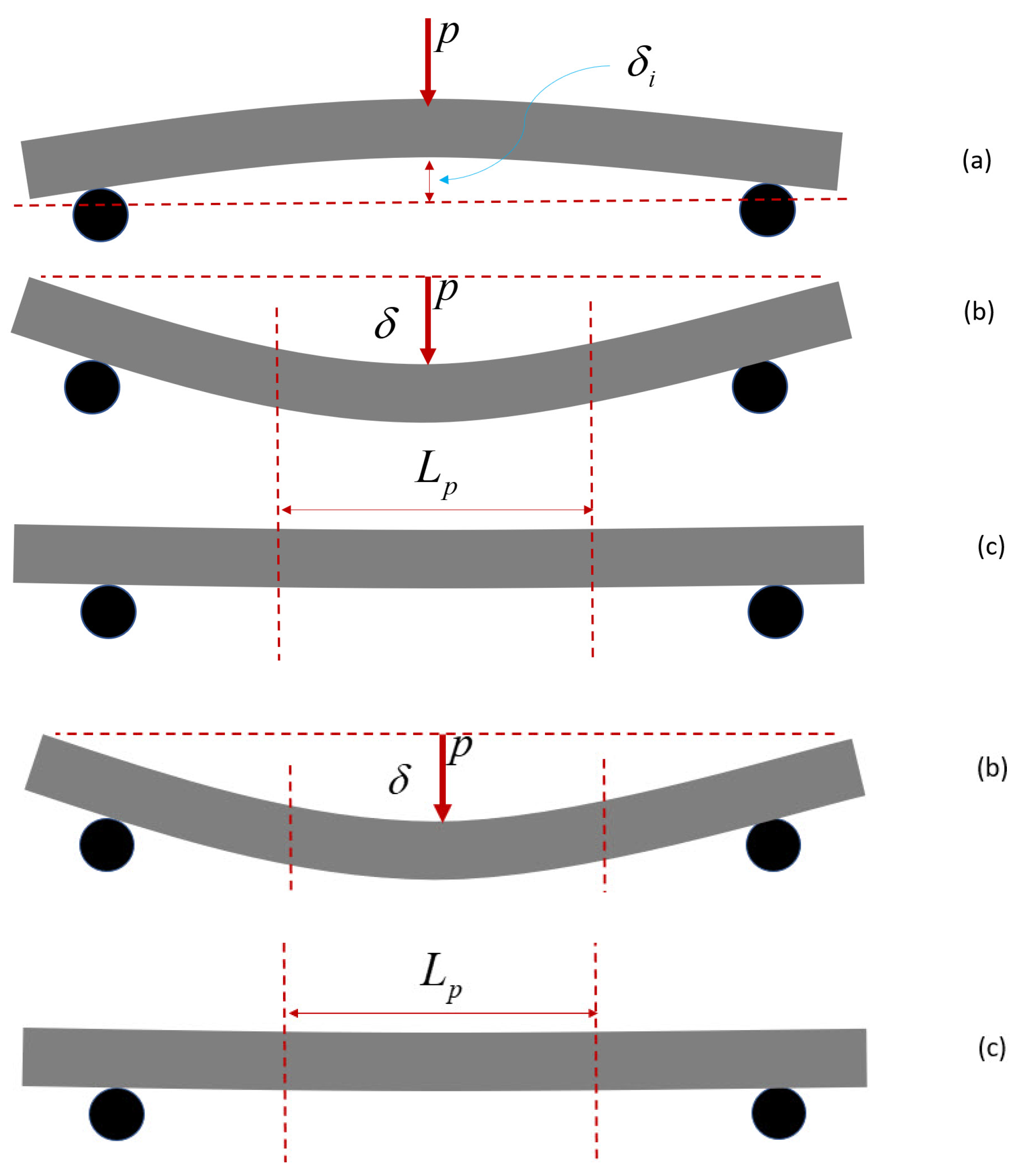
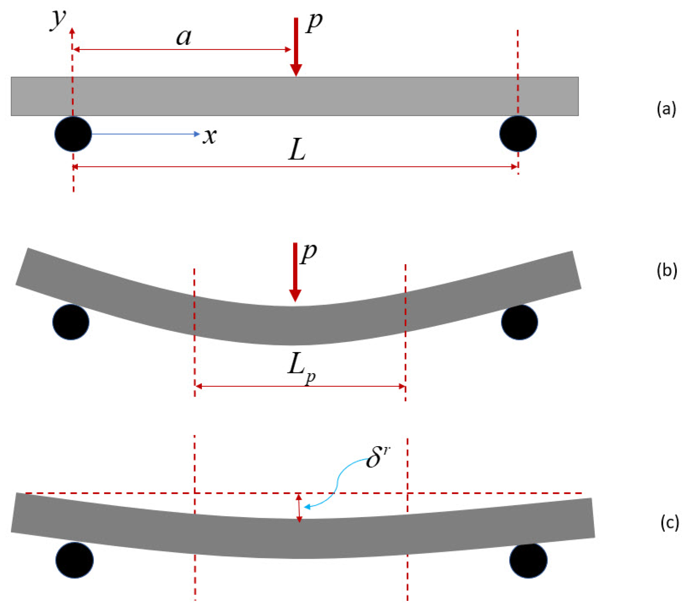
Mechanical shaft straightening is typically set up in a three-point bending mode, as illustrated in Figure 1. The load is applied at the location where the maximum straightness error has been identified using the simple supports arranged on both sides (see Figure 1a). The shaft is then bent under a straightening load with the shape illustrated in Figure 1b. If the load is large enough, then the yielding occurs within a certain range away from the loading position (Figure 1b). After the load is released, the shaft cannot revert to the initial convex shape and becomes straight (Figure 1c) if the amount of residual deflection due to the plastic deformation equals or is very close to the initial straightness error: (Figure 1a). Figure 1 depicts the whole process of the three-point bend straightening. The objective of this study was to develop an analytical computational method to analytically model the straightening process and predict the straightening load and the stroke displacements corresponding to straightness errors. The initial straightness error , as shown in Figure 1a, is usually in microns, i.e., 10−3 mm, which is negligible compared to the deflection (Figure 1b) under straightening load. Therefore, it is not necessary to include the initial straightness error in either the analytical model or the numerical FEA model. It indicates that the bend straightening modeling starts from a perfectly straight shaft (Figure 2a), and the load is applied at the location where has the highest straightness error . The shaft then deforms as the shape shown in Figure 2b. As the load is released, the springback occurs, and the shaft reaches an equilibrium status with a certain amount of residual deflection (Figure 2c). Without a precise analytical modeling method, it would then undergo a trial process until the residual deflection was close enough to the initial straightness error and the shaft met the distortion requirement.
2.2. Hardness-Based Material Model
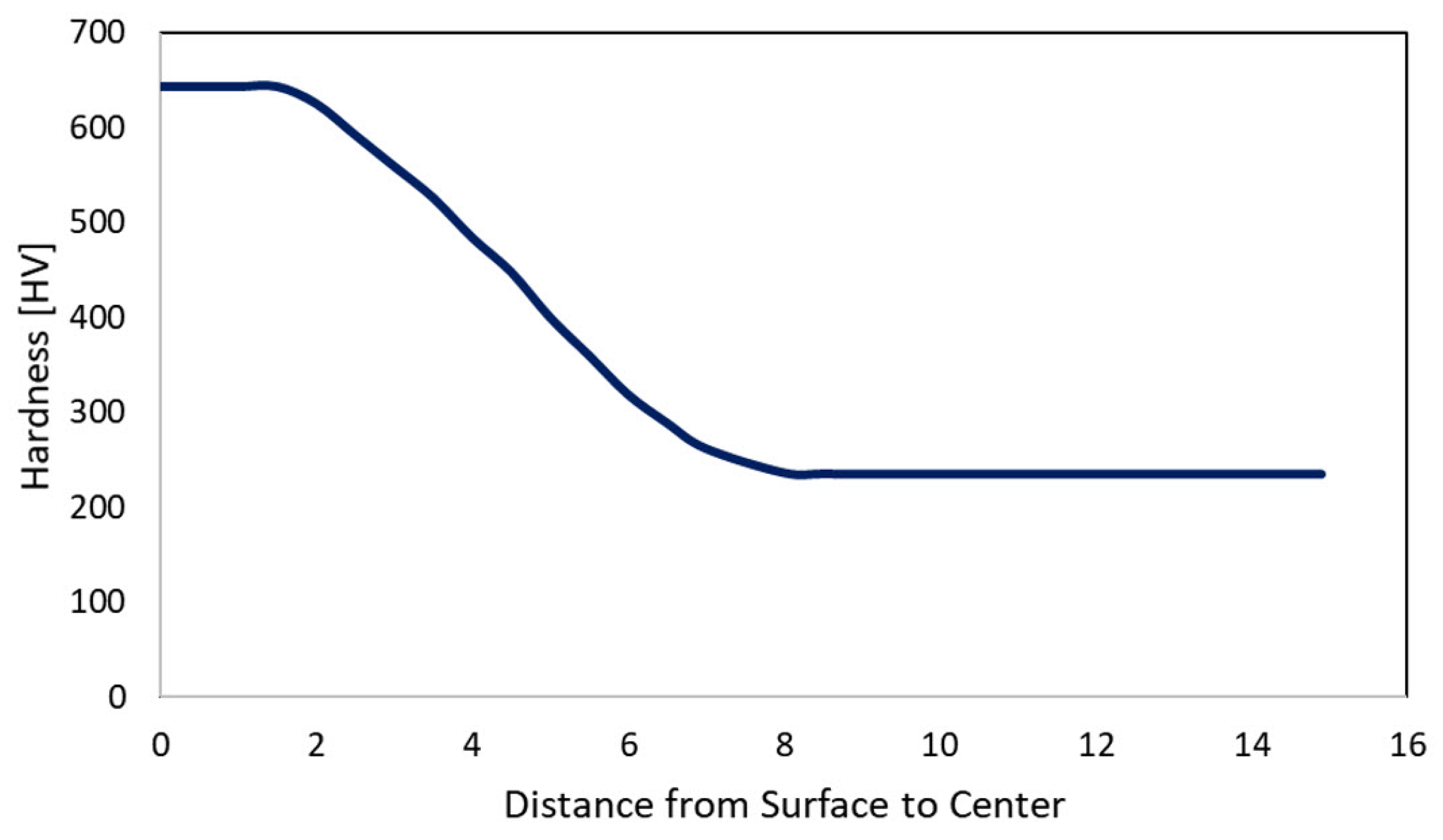
As mentioned previously, in the case of a hardened shaft, the hardness varies from surface to center, as depicted in Figure 3 (measurement provided by Barsoum and Khan et al. [11]). The hardness profile shown in Figure 3 was adopted for both analytical and numerical calculations in this study.
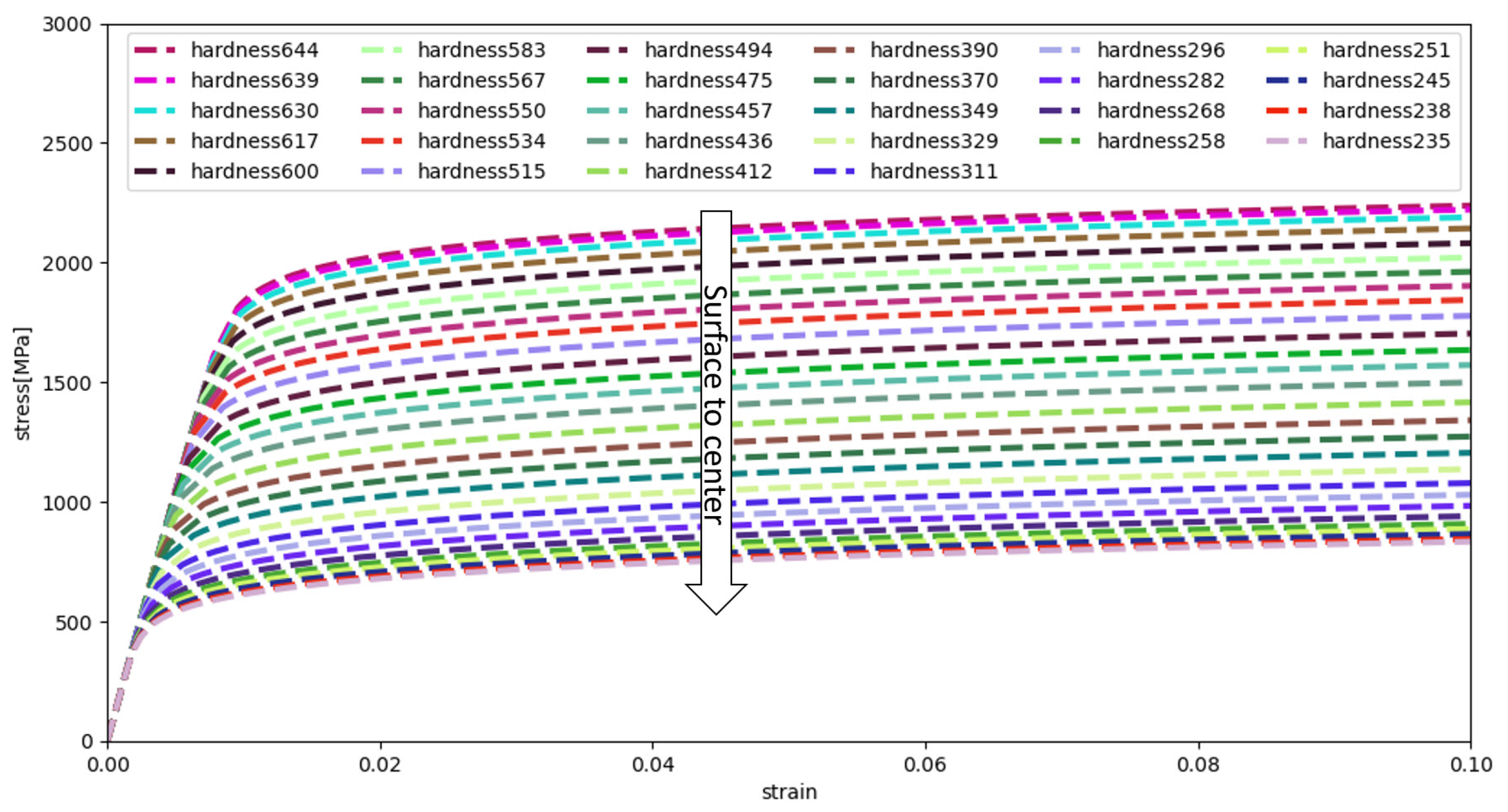
Moreover, Barsoum and Khan et al. [11] also provided the hardness-based materials for SAE 4140 steel expressed as a Ramberg–Osgood equation.
where E is Young’s modulus, and K and N denote the plastic modulus and the hardening exponent, which are functions of hardness and can be estimated based on the hardness-based material model proposed by Barsoum and Khan et al. [11]. For instance, with the hardness profile given in Figure 3, the stress–strain curves can be generated for any hardness from the core to the surface, as illustrated in Figure 4. The labels in Figure 4 correspond to the hardness profile shown in Figure 3. It can clearly be seen that the material on the surface has the highest yield stress and ultimate strength. The yield stress and ultimate strength can also be evaluated based on hardness [11]. It should be mentioned that the straightening process is quasi-static without considering temperature and strain rate. The Ramberg–Osgood material model was adopted in this study.
2.3. Shaft Deflection under Elastoplastic Bending
For a shaft under straightening load P at the position , as illustrated in Figure 2a, the reaction load in the left support can be expressed as
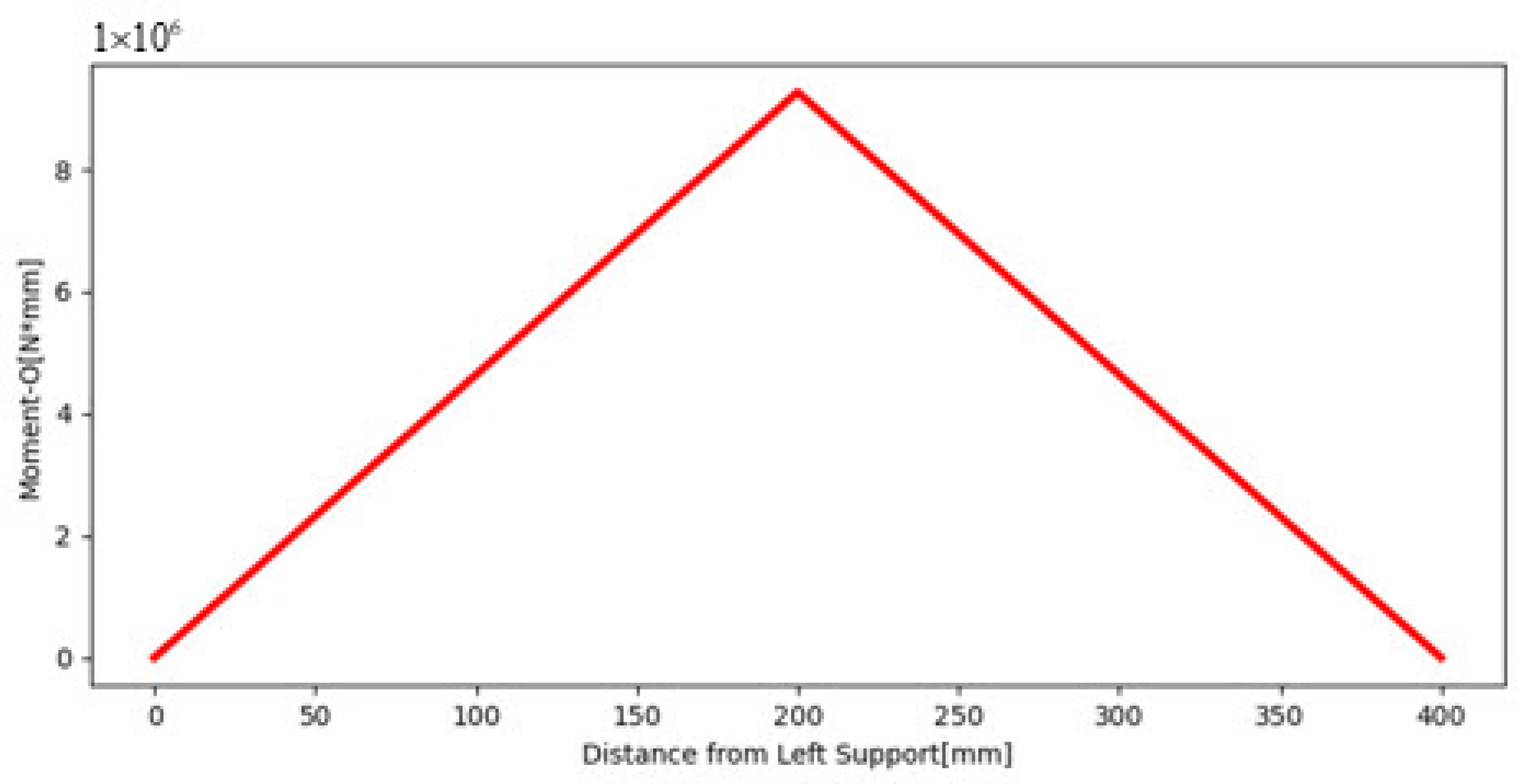
The moment can then be expressed as
The superscription “o” represents the moment due to loading for differentiation with the internal moment. In order to present the analytical development explicitly and visualize the intermediate products, an example of a straightening setup is provided in this section. The span is 400 mm, and the loading position (Figure 2) is mm. The straightening load is given as 92,680 N. The moment distribution (Equation (3)) can be depicted in Figure 5. It should be noted that the moment is linearly distributed and independent of the properties of materials.
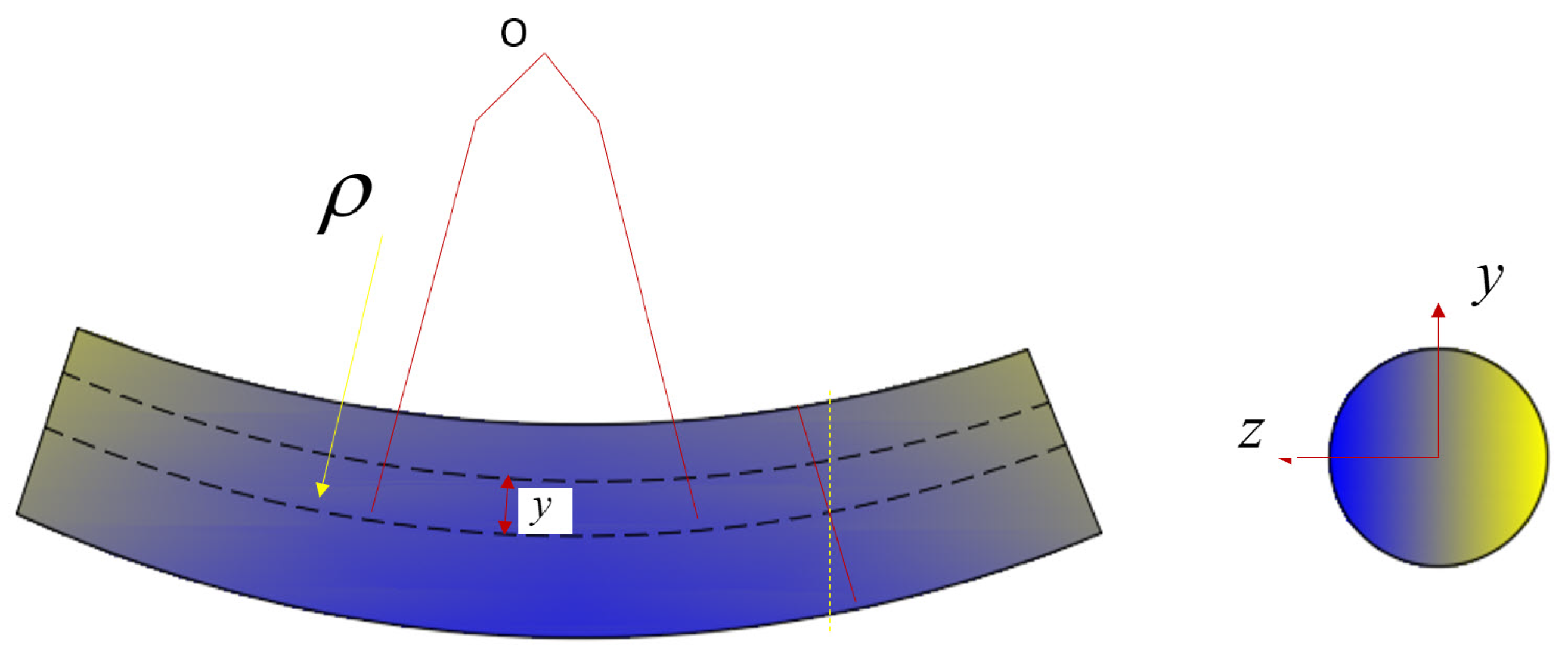
For linear elastic materials, the shaft deflection under three-point bending is quite simple to be determined by integrating the moment diagram, whereas to achieve the straightening effect as expected, the shaft has to be loaded into the plastic regime. Thus, the solutions for linear elastic materials cannot be applied directly. With the assumption ‘plane sections remain plane’ as shown in Figure 6, the strain within a cross section at a location can be expressed as
where is the curvature of the shaft under the bending load. The strain linearly varies in the y direction (Figure 6) but is independent of coordinate z. The purpose of introducing coordinate z in Equation (4) is to accommodate the material strength degradation from the surface to the center while evaluating stresses.
Taking advantage of the hardness-based material properties, substituting Equation (4) into Equation (1), the stress can be solved by inversing the Ramberg–Osgood equation below.
Then, the internal moments along the shaft under the bending load can be expressed in an integration form:
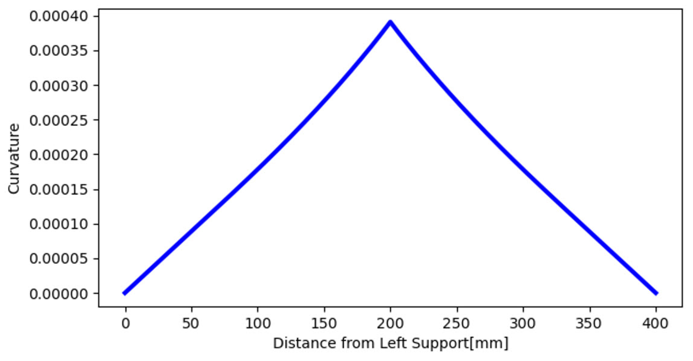
Given that the cross section of the shaft used in this study is circular, it is natural to perform integration under polar coordinate by replacing coordinates y and z (Figure 6) with r and , respectively. By equating the internal moment [Equation (6)] and moment [Equation (3)], the curvature can be solved, as is illustrated in Figure 7. If the deformation is within the linear regime, then the curvature will be distributed in the same manner as the moment diagram (Figure 5). It can clearly be seen in Figure 7 that the curvature is not linear as the moment diagram (Figure 5) in a range of about 100 mm to 300 mm, i.e., the length due to plastic deformation.
Since the deflection of the shaft under a straightening load is much less than the length of the case-hardened shaft due to its limited ductility on the hardened surface, the curvature can be estimated by
where is the deflection of the shaft. This can be obtained by integrating the curvature twice:
c and d are the two integration constants, which can be evaluated readily by the boundary conditions, i.e., at , and , . The shaft deflection will be plotted along with the FEA results in the next section. The deflection at the loading position, i.e., the stroke displacement (Figure 1b) can be calculated as .
2.4. Strain Evolution and Residual Deflection
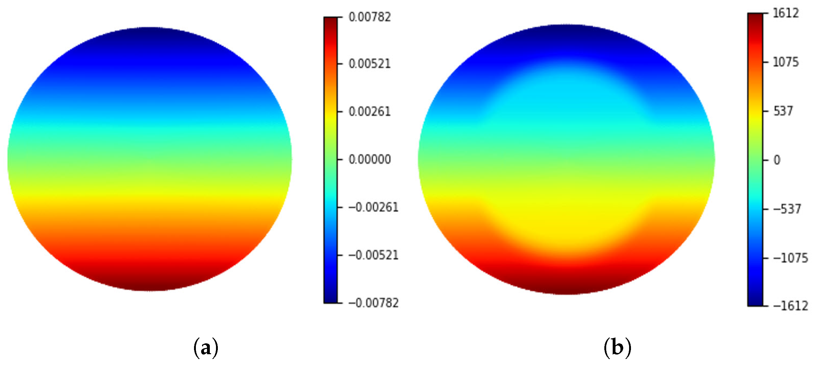
With the curvature obtained in the previous section, the total strain can be evaluated by Equation (4) and is shown in Figure 8a at the cross section where the load is applied. Correspondingly, the stress can be evaluated by Equation (5) and is illustrated in Figure 8b. It can be seen that the total strain (Figure 8) distributes linearly in the y direction and does not vary in the z direction as expected. Compared to strain distribution, stress is not linearly distributed in the y direction and is not constant in the z direction, as illustrated in Figure 8b, because of nonuniform material properties.
It should be noted that total strain (Figure 8a) contains both elastic and plastic strain components for the cross sections within . The plastic strain can be calculated by subtracting the yield strain . If the total strain is smaller than the yield strain, no yield occurs. Then, the plastic strain can be expressed as
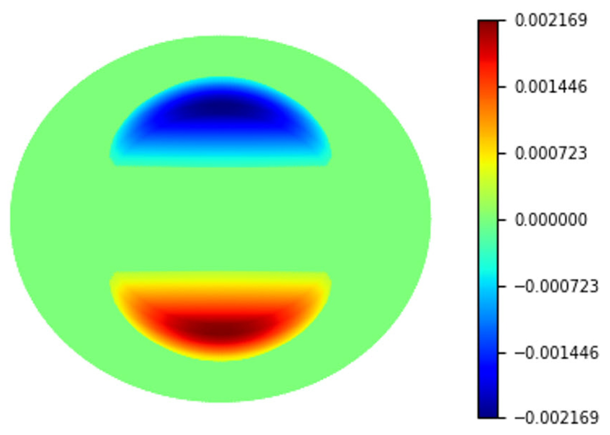
If the materials of the shaft are uniform, yielding starts from the surface where the highest strain is located. However, this is not the case for case-hardened shafts, as the highest yield stress is on the shaft surface (Figure 4). Considering the same cross-section as Figure 8a, the plastic strain was evaluated and distributed as two half-moon shapes (Figure 9) for the hardening profile, as is shown in Figure 3. Figure 9 also indicates that the surrounding area of the half-moons did not reach yield for the load amplitude applied in the current example. As the straightening load increases, the plastic areas would expand.
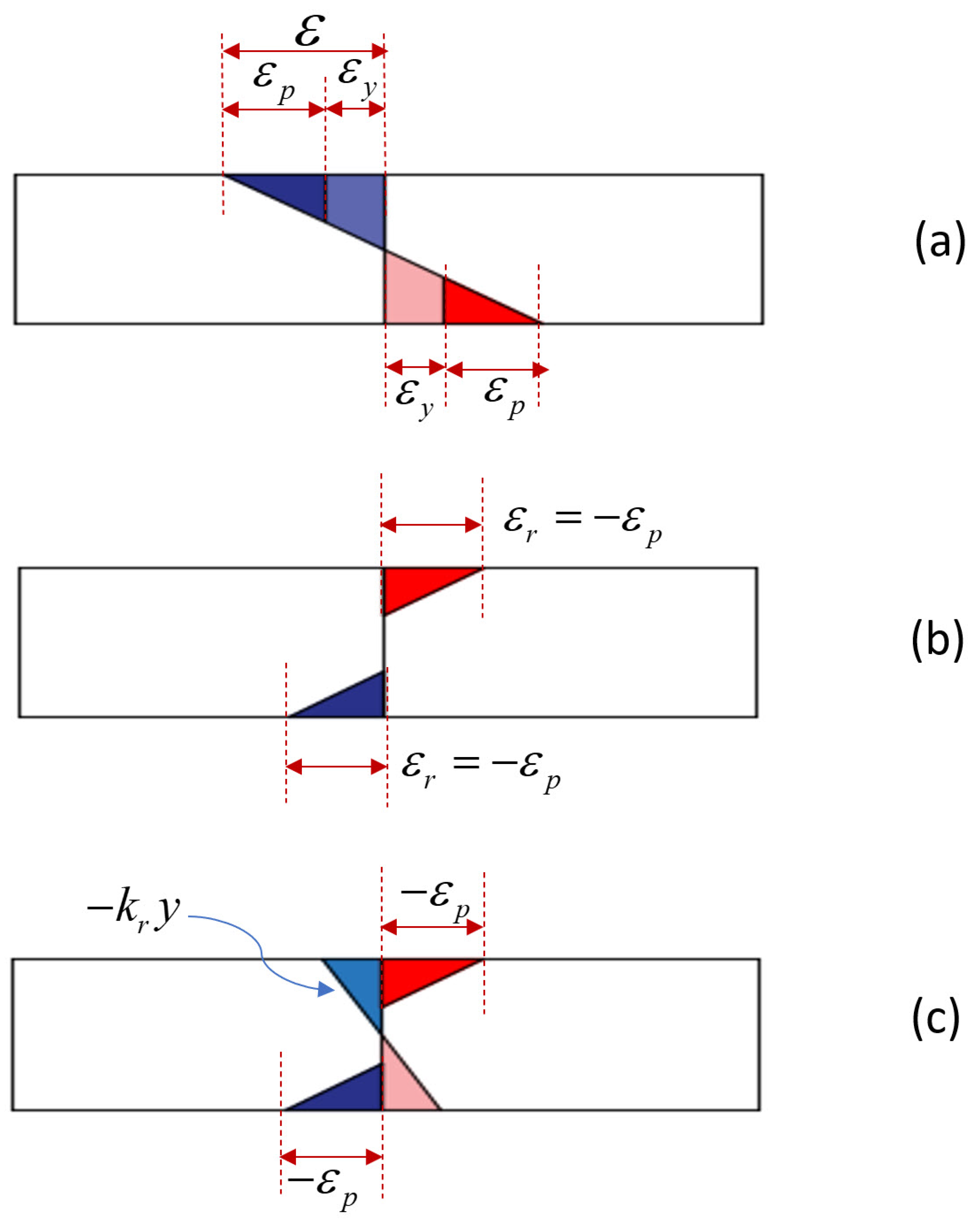
In order to simply illustrate the evolution of strain in the straightening process, the materials of the shaft are assumed to be uniform with the same yield strain . Thus, the total strain and plastic strain can be depicted as in Figure 10a. Once the straightening load reaches the command load amplitude, it will be released, and the shaft undergoes springback. Assuming that the shaft is restored to the original straight shape as the load is released, the elastic strains are reversible, whereas the plastic strain (Figure 10a) becomes residual strain with opposite signs as shown in Figure 10b. It can be seen clearly that Figure 10b exhibits a nonequilibrium state with a resultant residual moment. The shaft has to bend until a new equilibrium status is achieved. Denoting the curvature at the equilibrium state as , the strain through the cross section can be described as similar to Equation (4) and depicted in Figure 10c, and it can be seen the residual moment is equilibrated. The resultant residual strain of the shaft at the equilibrium state can be expressed as
By substituting strain Equation (10) into the Ramberg–Osgood stress–strain model [Equation (1)], the residual stress can be evaluated. Then, the residual moment can be expressed as,
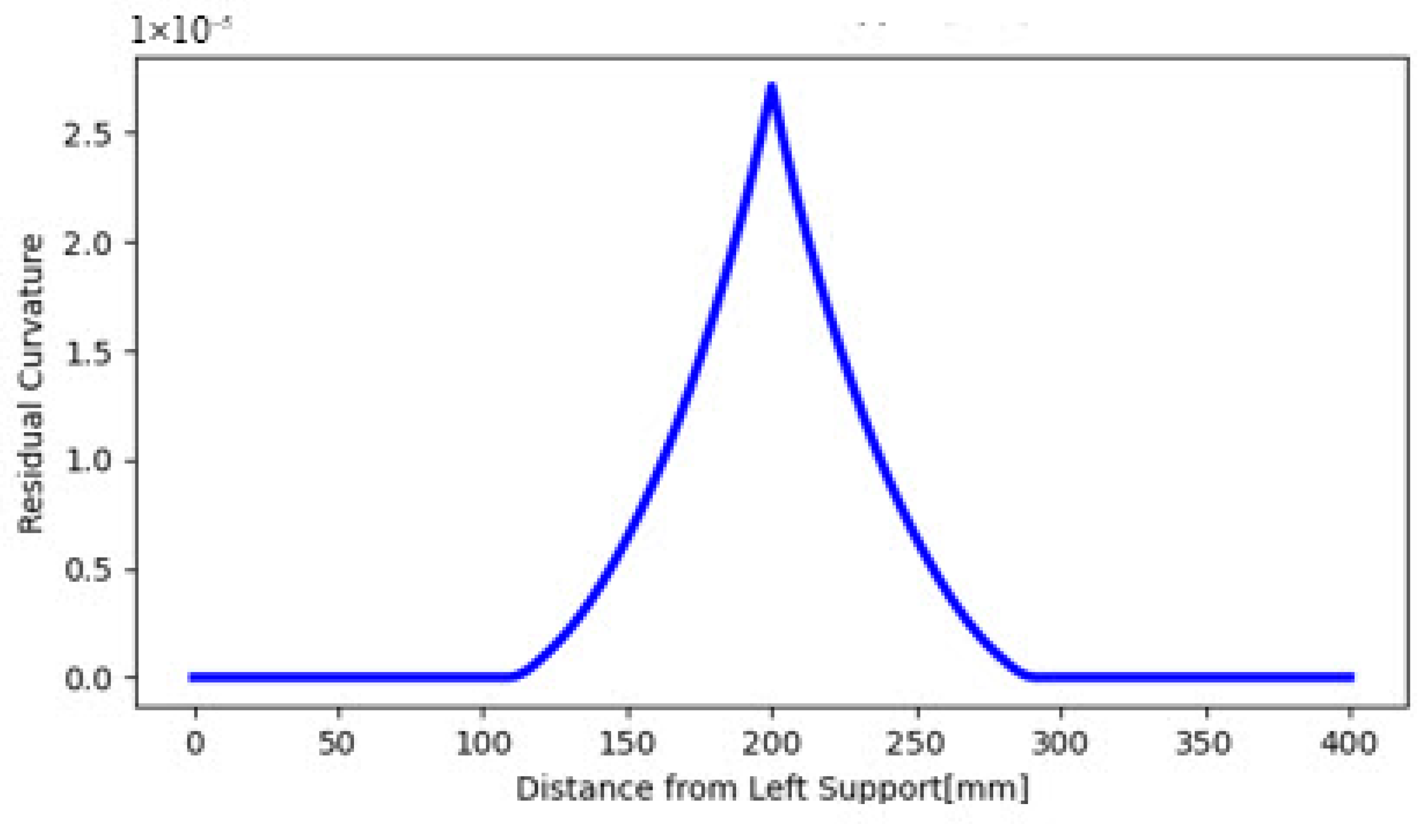
Similar to Equation (6), Equation (11) will be integrated under the polar coordinate. Since the residual stress and the residual moment must be self-equilibrating, the residual moment at each cross section equals zero, i.e., . Therefore, the residual curvature can be obtained and illustrated in Figure 11. It (Figure 11) indicates that the highest residual curvature is found where the straightening load is applied, and the plastic deformation starts from about mm to mm.
Since the residual deflection is small, the relation between the residual curvature and residual deflection similar to Equation (7) still holds,
Eventually, by integrating the residual curvature twice, the residual deflection can be obtained and expressed as,
where and are the two integration constants and can be evaluated by the two boundary conditions, i.e., at , , and , . The residual deflection curves will be presented in the next section. The residual deflection at the loading position (Figure 2c) was obtained as .
3. Numerical Simulation
3.1. Finite Element Model
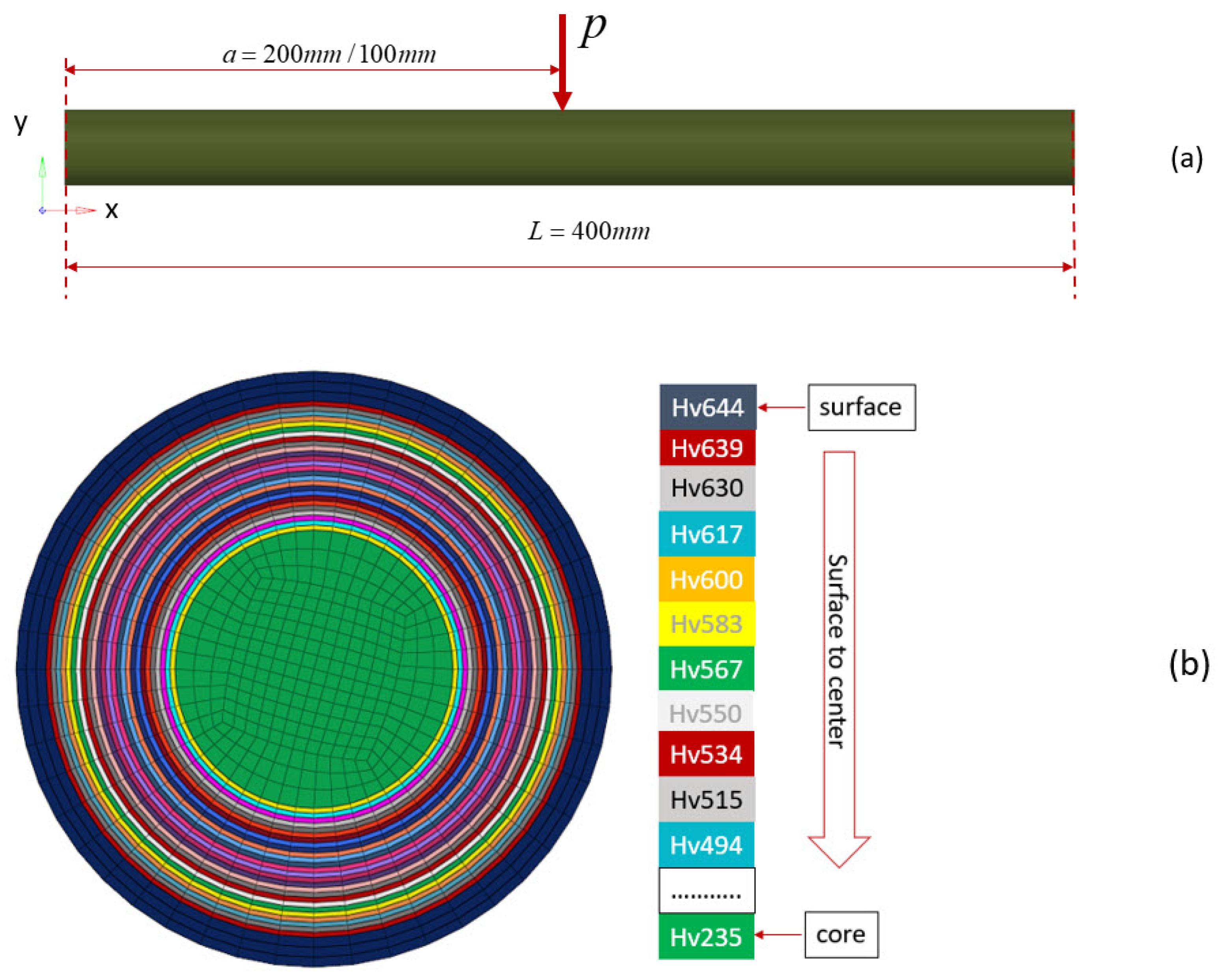
In order to validate the analytical method developed in this study, finite element analysis was conducted using Abaqus. A shaft with a diameter of 44 mm representing a typical size in the driveline system was selected, and the span L between the two supports (Figure 12a) was 400 mm. To verify the robustness of the analytical model developed in this study, two straightening setups were considered. In the first, the load was applied in the middle, i.e., mm, and in the other, the load was applied at a quarter of the span, i.e., mm. The end conditions representing anvils are modeled as a simple support. In order to avoid shear locking under bending load, the incompatible mode eight-node brick element type (C3D8I) was selected. The mesh size in the shaft axial direction was 2 mm. The cross sections of the shaft were modeled as layers corresponding to the hardness profile, as shown in Figure 3, and each layer represented a specific hardness illustrated in Figure 12b with a colored mapping. The hardness-based material properties presented in Figure 4 are assigned to the corresponding layers in the finite element model. All of the load cases conducted are listed in Table 1.
3.2. Straightening Load in the Middle
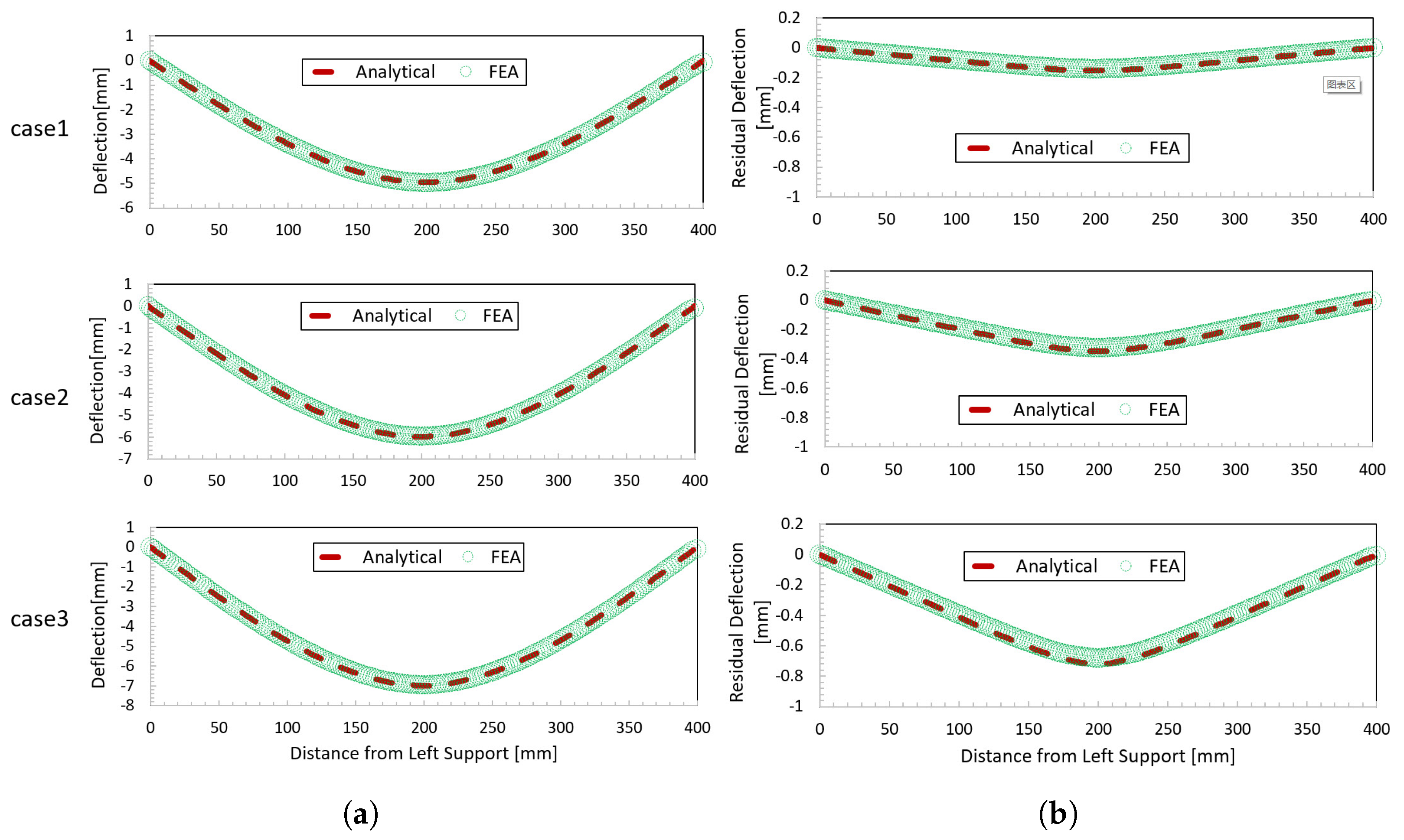
For cases 1–3 as listed in Table 1, the load was applied at the middle of the shaft. Three straightening loads were applied in order to achieve small, medium, and large plastic deformation. As illustrated in Figure 13a, the analytical shaft deflections curve evaluated by Equation (8) agreed very well with the FEA results. The predicted stroke displacements (deflection at the loading position) were almost identical to the FEA results (see Table 2). The analytically predicted residual deflection curve resulting from Equation (13) was slightly higher than the FEA results (see Figure 13b). At the loading positions, the residual deflections were about 5–7% higher than the FEA results, which were on the conservative side and could avoid over-straightening.
3.3. Straightening Load at the Quarter
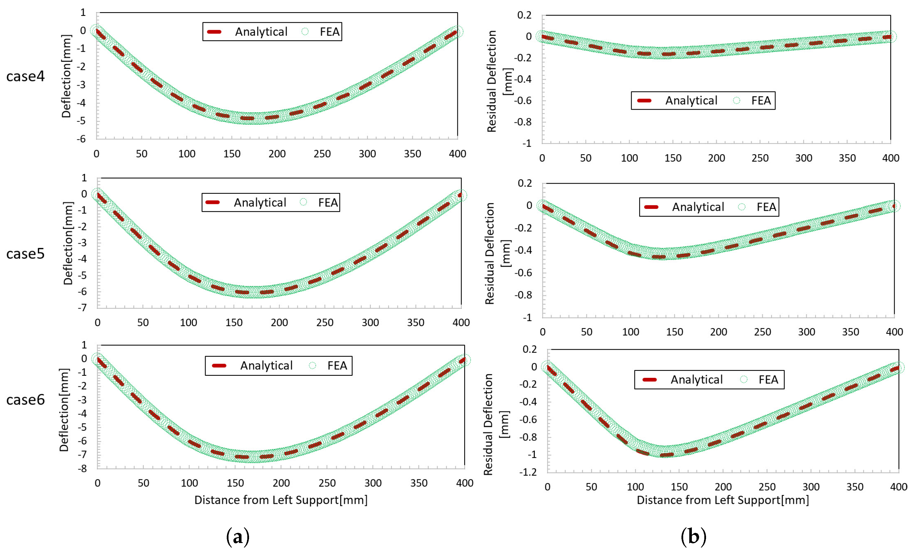
In the previous section, it can be seen that the analytical solutions match the FEA results when the straightening load is applied at the middle of the shaft. In order to verify the robustness of the analytical method, another group of virtual tests, i.e., load cases 4–6, with the load applied at the quarter of shafts, were carried out. As illustrated in Figure 14a, the analytical shaft deflections generated by Equation (8) perfectly overlap with the FEA results regardless of the use of small or large loads. Similar to load cases 1–3, the analytical residual deflection curve evaluated by Equation (13) is slightly higher than the FEA results (Figure 14b). The stroke displacements at the loading position are approximately 3–5.5% higher than those of the FEA results (see Table 3). It should be noted that the maximum residual deflection does not occur where the load is applied. As observed from Figure 14b, it is about 30 mm away from the load position toward the right end and varies as load amplitude changes. The residual deflection at the load position is about 5–8% lower than the maximum. Therefore, in practice, the preferred loading position should be in the middle of the span between anvils.
4. Practical Application
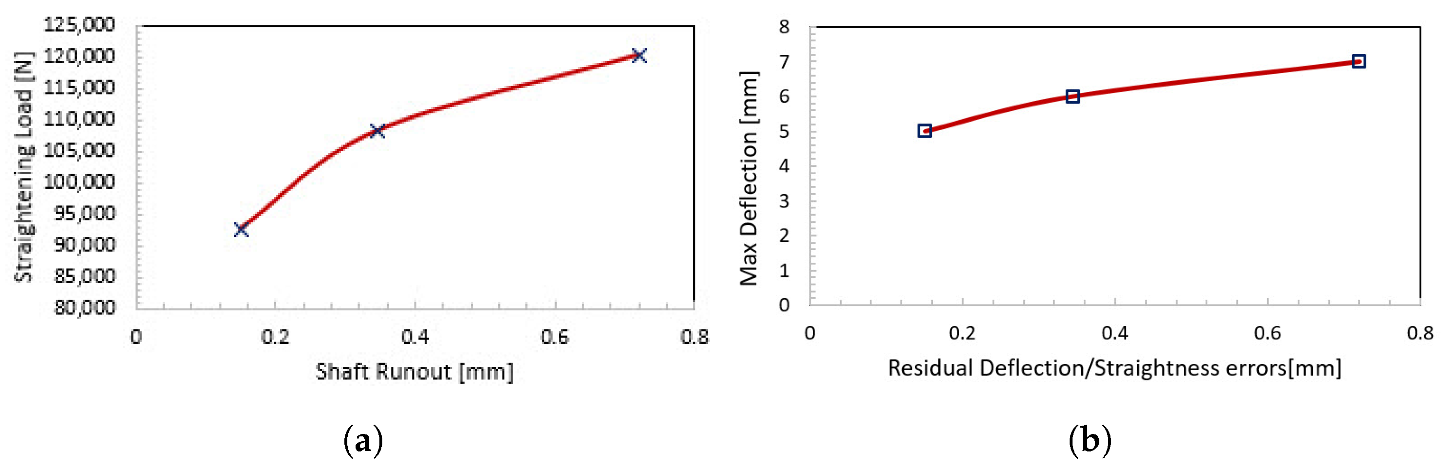
The accuracy and robustness of the analytical method developed in this study have been validated in the previous section. Straightening cycles will be significantly reduced if stroke displacements are predicted in advance by applying this method in practice. Although the theoretical method was developed in load control conditions, it can be applied for displacement control as well. For instance, taking advantage of the results from cases 1–3, the relationship between either straightening load or stroke displacement and shaft residual deflection can be established as shown in Figure 15. Note that residual deflections should ideally have equal shaft straightness errors, i.e., straightening effect to be achieved as expected. Therefore, if the straightness errors of the shaft have been measured and the locations of the anvils and loading hammer are set, e.g., as the same virtual tests in this study, the straightening load can be readily found by Figure 15a. In the same manner, the stroke displacement can be determined by Figure 15b. The straightening then can be set up as either load or displacement control. In the case that the straightening load is not applied in the middle of the shaft, the application strategy is the same as the load applied in the middle of the shaft. In practice, to achieve better results, more load cases need to be prerun in order to establish the mappings as in Figure 15. It is also worth noting that the analytical development was based on a case-hardened shaft with smooth geometry. Finite element calculations are necessary for a shaft with grooves.
5. Concluding Remarks
In this paper, an advanced theoretical straightening model for case-hardened shafts was developed. Its effectiveness and robustness were then validated by a systematic numerical virtual test. Considering current manufacturing conditions in the industry, an application strategy was proposed. The following conclusions can be drawn:
- The analytical straightening model developed in this study can predict stroke displacement and residual deflection effectively. The slight discrepancy between analytical solutions and FEA results might be attributed to the fact that the hardness profile used in the analytical model is continuous and transitions much more smoothly than in the layered finite element model.
- The analytical straightening model can be utilized for any three-point bending setup. As the straightening load is off the middle of the shaft, the maximum residual deflection occurs at a certain distance away from the loading position, which varies with the loading position and load amplitude.
- Once a straightening setup is determined, the relationship between load or stroke displacement and measured straightness error can be established using the theoretical model developed in this study. It will improve the efficiency of straightening and avoid over-straightening in practice.
Funding
This research received no external funding.
Data Availability Statement
All data are contained within the article.
Conflicts of Interest
The authors declare no conflict of interest.
References
- Nasruddin, M.; Artady, H. Case study of straightening methods for bent shaft 1.25 mm on hip turbine rotor pacitan steam power plant# 1. In Proceedings of the 2019 International Conference on Technologies and Policies in Electric Power & Energy, Yogyakarta, Indonesia, 21–22 October 2019; pp. 1–5. [Google Scholar]
- Li, J.; Xiong, G.L.; Zhou, H.J. Process modeling and stroke calculation for shaft straightening. J. Heave Mach. 2004, 6, 41–44. [Google Scholar]
- Li, J.; Zou, H.; Xiong, G.L. Establishment and application of load-deflection model of press straightening. In Key Engineering Materials; Trans Tech Publications Ltd.: Stafa-Zurich, Switzerland, 2004; Volume 274, pp. 475–480. [Google Scholar]
- Lu, H.; Ling, H.; Leopold, J.; Zhang, X.; Guo, C. Improvement on straightness of metal bar based on straightening stroke-deflection model. Sci. China Ser. Technol. Sci. 2009, 52, 1866–1873. [Google Scholar] [CrossRef]
- Lu, H.; Zang, Y.; Zhang, X.; Zhang, Y.; Li, L. A general stroke-based model for the straightening process of d-type shaft. Processes 2020, 8, 528. [Google Scholar] [CrossRef]
- Pei, Y.C.; Wang, J.W.; Tan, Q.C.; Yuan, D.Z.; Zhang, F. An investigation on the bending straightening process of d-type cross section shaft. Int. J. Mech. Sci. 2017, 131, 1082–1091. [Google Scholar] [CrossRef]
- Natarajan, A.; Peddieson, J. Simulation of beam plastic forming with variable bending moments. Int. J. Non-Linear Mech. 2011, 46, 14–22. [Google Scholar] [CrossRef]
- Kim, S.C.; Chung, S.C. Synthesis of the multi-step straightness control system for shaft straightening processes. Mechatronics 2002, 12, 139–156. [Google Scholar] [CrossRef]
- Shamsaei, N.; Fatemi, A. Deformation and fatigue behaviors of case-hardened steels in torsion: Experiments and predictions. Int. J. Fatigue 2009, 31, 1386–1396. [Google Scholar] [CrossRef]
- McClaflin, D.; Fatemi, A. Torsional deformation and fatigue of hardened steel including mean stress and stress gradient effects. Int. J. Fatigue 2004, 26, 773–784. [Google Scholar] [CrossRef]
- Barsoum, I.; Khan, F.; Barsoum, Z. Analysis of the torsional strength of hardened splined shafts. Mater. Des. 2014, 54, 130–136. [Google Scholar] [CrossRef]
Figure 1.
Illustration of the shaft bend straightening process: (a) distorted shaft to be straightened; (b) shaft deflected under straightening load; (c) straightened shaft.
Figure 1.
Illustration of the shaft bend straightening process: (a) distorted shaft to be straightened; (b) shaft deflected under straightening load; (c) straightened shaft.

Figure 2.
Analytically modeled straightening process: (a) an ideally straight shaft subjected to a bending load; (b) deflected shaft under load; (c) unloaded shaft with residual deflection.
Figure 2.
Analytically modeled straightening process: (a) an ideally straight shaft subjected to a bending load; (b) deflected shaft under load; (c) unloaded shaft with residual deflection.

Figure 3.
A typical hardness profile resulting from induction hardening.

Figure 4.
Hardness-based true stress–strain curves.

Figure 5.
Bending moment diagram.

Figure 6.
Shaft deformation under elastoplastic bending.

Figure 7.
Curvature distribution along shaft axis as loaded.

Figure 8.
Stress and strain distribution at the location of loading: (a) strain distribution; (b) stress [MPa] distribution.
Figure 8.
Stress and strain distribution at the location of loading: (a) strain distribution; (b) stress [MPa] distribution.

Figure 9.
Plastic strain in shaft axial direction.

Figure 10.
Strain evolution in the straightening process: (a) strain distribution under loading; (b) residual strain distribution without residual deflection; (c) resultant residual strain with residual deflection.
Figure 10.
Strain evolution in the straightening process: (a) strain distribution under loading; (b) residual strain distribution without residual deflection; (c) resultant residual strain with residual deflection.

Figure 11.
Residual curvature.

Figure 12.
Finite element model: (a) overall dimensions; (b) cross-section of layered finite element model with hardness mapping.
Figure 12.
Finite element model: (a) overall dimensions; (b) cross-section of layered finite element model with hardness mapping.

Figure 13.
Shaft deflections for the load applied in the middle of shaft cases 1–3: (a) shaft deflection under loading; (b) residual deflection.
Figure 13.
Shaft deflections for the load applied in the middle of shaft cases 1–3: (a) shaft deflection under loading; (b) residual deflection.

Figure 14.
Shaft deflections for load applied at the quarter of shaft cases 4–6: (a) shaft deflection under loading; (b) residual shaft deflection.
Figure 14.
Shaft deflections for load applied at the quarter of shaft cases 4–6: (a) shaft deflection under loading; (b) residual shaft deflection.

Figure 15.
Plots of straightening load and stroke displacement in terms of residual deflection: (a) straightening load vs. residual deflection; (b) stroke displacement vs. residual deflection.
Figure 15.
Plots of straightening load and stroke displacement in terms of residual deflection: (a) straightening load vs. residual deflection; (b) stroke displacement vs. residual deflection.


Table 1.
Load cases.
| a [mm] | L [mm] | P [N] | |
|---|---|---|---|
| Case 1 | 200 | 400 | 92,680 |
| Case 2 | 200 | 400 | 108,200 |
| Case 3 | 200 | 400 | 120,360 |
| Case 4 | 100 | 400 | 129,910 |
| Case 5 | 100 | 400 | 154,990 |
| Case 6 | 100 | 400 | 171,790 |
Table 2.
Comparison of the analytical and FEA results of cases 1–3.
| Analytical Solution [mm] | FEA Results [mm] | |||
|---|---|---|---|---|
| Stroke Displacement | Residual Deflection | Stroke Displacement | Residual Deflection | |
| Case 1 | −4.95 | −0.151 | −4.97 | −0.14 |
| Case 2 | −5.97 | −0.345 | −5.97 | −0.325 |
| Case 3 | −6.98 | −0.72 | −6.96 | −0.681 |
Table 3.
Comparison of analytical and FEA results of cases 4–6.
| Analytical Solution [mm] | FEA Results [mm] | |||
|---|---|---|---|---|
| Stroke Displacement | Residual Deflection | Stroke Displacement | Residual Deflection | |
| Case 4 | −3.93 | −0.162 | −3.92 | −0.154 |
| Case 5 | −4.95 | −0.456 | −4.9 | −0.431 |
| Case 6 | −5.95 | −1 | −5.89 | −0.964 |
Disclaimer/Publisher’s Note: The statements, opinions and data contained in all publications are solely those of the individual author(s) and contributor(s) and not of MDPI and/or the editor(s). MDPI and/or the editor(s) disclaim responsibility for any injury to people or property resulting from any ideas, methods, instructions or products referred to in the content. |
© 2023 by the author. Licensee MDPI, Basel, Switzerland. This article is an open access article distributed under the terms and conditions of the Creative Commons Attribution (CC BY) license (https://creativecommons.org/licenses/by/4.0/).
Share and Cite
MDPI and ACS Style
Xing, S. Analytical Modeling for Mechanical Straightening Process of Case-Hardened Circular Shaft. Appl. Mech. 2023, 4, 715-728. https://doi.org/10.3390/applmech4020036
AMA Style
Xing S. Analytical Modeling for Mechanical Straightening Process of Case-Hardened Circular Shaft. Applied Mechanics. 2023; 4(2):715-728. https://doi.org/10.3390/applmech4020036
Chicago/Turabian StyleXing, Shizhu. 2023. "Analytical Modeling for Mechanical Straightening Process of Case-Hardened Circular Shaft" Applied Mechanics 4, no. 2: 715-728. https://doi.org/10.3390/applmech4020036