A Numerically Efficient Method to Assess the Elastic–Plastic Strain Energy Density of Notched and Imperfective Cast Steel Components

Abstract

The fatigue strength of cast steel components is severely affected by manufacturing process-based bulk and surface imperfections. As these defect structures possess an arbitrary spatial shape, the utilization of local assessment methods is encouraged to design for service strength. This work applies the elastic–plastic strain energy density concept to study the fatigue strength properties of a high-strength cast steel alloy G12MnMo7-4+QT. A fatigue design limit curve is derived based on non-linear finite element analyses which merges experimental high-cycle fatigue results of unnotched and notched small-scale specimens tested at three different stress ratios into a unique narrow scatter band characterized by a scatter index of $1:T_{\Delta {\overline{W}}^{\left(t\right)}}=2.43$. A comparison to the linear–elastic assessment conducted in a preceding study reveals a significant improvement in prediction accuracy which is assigned to the consideration of the elastic–plastic material behaviour. In order to reduce computational effort, a novel approximation is presented which facilitates the calculation of the elastic–plastic strain energy density based on linear–elastic finite element results and Neuber’s concept. Validation of the assessment framework reveals a satisfying agreement to non-linear simulation results, showing an average root mean square deviation of only approximately eight percent in terms of total strain energy density. In order to study the effect of bulk and surface imperfections on the fatigue strength of cast steel components, defect-afflicted large-scale specimens are assessed by the presented elastic–plastic framework, yielding fatigue strength results which merge into the scatter band of the derived design limit curve. As the conducted fatigue assessment is based solely on linear–elastic two-dimensional simulations, the computational effort is substantially decreased. Within the present study, a reduction of approximately 400 times in computation time is observed. Hence, the established assessment framework presents an engineering-feasible method to evaluate the fatigue life of imperfective cast steel components based on rapid total strain energy density calculations.

1. Introduction

Due to strict environmental regulations, modern production strives for a lightweight design of mechanical components [1]. Engineering tools such as topology optimization represent feasible methods to combine application-tailored parts and economic production [2,3]. Such designs often lead to complex-shaped components possessing thin-walled cross-sections and therefore high loading conditions of their respective parts. In order to simultaneously fulfil the requirements in terms of manufacturability and fatigue strength of these complex structures, high-strength cast steel alloys are suitable engineering materials due to their favourable mouldability and high load-bearing capacities. The chemical composition of such alloys facilitates their utilization in welded hybrid constructions such as bogie frames in railway applications, consisting of complexly shaped cast components and standardized parts with various beam geometries. However, despite the latest advances in numerical simulations in the casting process [4,5,6,7,8], the formation of manufacturing process-based shrinkage imperfections within highly loaded sections cannot be fully prevented. Due to high-volume contraction, these spatial defect structures often reach dimensions of several millimetres [9,10,11,12]. Hence, the fatigue strength of the respective components is significantly affected by the presence of such macroscopic imperfections [13,14,15,16,17].

Design guidelines such as the commonly utilised guideline FKM (Forschungskuratorium Maschinenbau) [18] propose safety factors to consider the detrimental effect of defects on the fatigue strength of cast steel components. These safety factors only consider the applied methods of non-destructive testing during quality control of respective cast steel structures, fully neglecting the geometrical shape and location of inherent imperfections. Hence, the application of such safety factors often results in conservatively designed, overweight components which often repeal the advantages achieved by topology optimization. In order to take the geometrical shape of casting defects into account, the standard ASTM E446 [19] provides reference radiographs depicting representative imperfection geometries. Defect structures are classified into categories which reflect their causes of appearance, such as slag inclusions or shrinkage imperfections. Within a category, each reference radiograph represents a certain severity grade which is mainly defined based on the size and amount of the depicted imperfections. During the design process, specific combinations of defect category and severity grade are denoted as not acceptable for operation. Utilizing this defect classification system, assessment of defect-afflicted cast steel components is simply conducted by comparison of X-ray images of corresponding components to the reference radiographs. If occurring imperfections match a defect class denoted as non-acceptable, the component must be repaired or even scrapped and a new part has to be manufactured, increasing cost and time expenses significantly. A major drawback of this assessment method lies in the sole consideration of the defect geometry, fully neglecting its location in the assessed component. This circumstance implies that the existence of a certain imperfection could lead to the rejection of a manufactured component, even if it is located in a cross-section subjected to negligible stress. Furthermore, the interpretation of radiographs is a highly subjective task which depends strongly on the experience of the responsible personnel [20]. Hence, the same imperfection could be classified as either acceptable or non-acceptable, depending on the subjective interpretation of the non-destructive testing results.

In order to provide an objective quantitative assertion about the effect of imperfections on the fatigue behaviour of cast steel components, local assessment methods which consider the shape and location of inherent defect structures should be applied.

Defect structures such as shrinkage porosity networks induce a locally acting multiaxial stress state. Due to the ductile material behaviour of cast steel alloys, the resulting local loading conditions cause elastic–plastic deformation in the vicinity of each imperfection. Considering cyclic loading of notched or defect-afflicted parts, the non-linear material response results in mean stress relaxation [21,22,23,24] which alters the cyclic loading hysteresis until stabilization of the material behaviour. This stabilization process leads to the formation of a local effective stress ratio $R_{eff}$, similar to the case of residual stresses that interact with stresses induced by external loading [25,26]. In order to consider non-linear deformations during finite element analysis, the constitutive material equation provides the connection between strains and stresses [27]. Several elastic–plastic models are reported in the literature to include plasticity effects during cyclic loading such as Bauschinger’s effect or ratcheting [28,29]. A common constitutive model to describe the inelastic behaviour of metallic materials is given by Chaboche [30]. The approach presents a combined hardening model which considers isotropic as well as non-linear kinematic hardening and is therefore capable of describing the evolution of size and position of the yield surface in the space of stresses. The evaluation of the applicable constitutive model parameters is a well-researched topic and comprehensively published [31,32,33,34,35]. The application of combined hardening material models covers a broad variety of advanced research topics such as creep-fatigue analysis at elevated temperatures or uni- to multiaxial loading conditions in static and dynamic structural integrity analysis [36,37,38,39].

Dealing with the fatigue analysis of defect-afflicted ductile cast steel components, the non-linear deformation behaviour can be implemented into the assessment procedure to consider the cyclic evolution of the multiaxial stress state induced by the respective imperfections. This necessitates an assessment methodology capable of considering local plastic strains in order to accurately describe their influence on fatigue strength. The strain energy density (SED) concept presents a local fatigue assessment method that is utilised to assess arbitrarily shaped notches subjected to varying loading conditions. Fatigue failure occurs if the SED averaged over the control volume $\mathsf{\Omega }$ reaches a critical value [40]. Herein, $\mathsf{\Omega }$ represents a finite volume in the vicinity of a stress concentrator and is described by the material-dependent control radius $R_c$ and the notch geometry [41]. Figure 1 visualizes the definition of $\mathsf{\Omega }$ for sharp and blunt V-notches, characterized by the notch opening angle $2\alpha$ and the notch root radius $\rho$ [40,42].

In the case of a sharp notch, the control volume is centred in the notch root and takes the shape of a circle segment. Dealing with blunt notches as a generalized case, the control volume takes the form of a crescent shape with its centre located at a distance $r_0$ from the notch root, where $r_0$ is a function of $2\alpha$ and $\rho$ [40,42].

In analogy to strains, the total cyclic strain energy density $\Delta W^{\left(t\right)}$ can be defined as the superposition of an elastic $\Delta W^{\left(e\right)}$ and plastic contribution $\Delta W^{\left(p\right)}$ as given in Equation (1) [43].

$$\Delta W^{\left(t\right)}=\Delta W^{\left(e\right)}+\Delta W^{\left(p\right)}$$

(1)

Equation (1) also holds true when dealing with SED values averaged over the control volume which are denoted by an overline accent, for example $\Delta {\overline{W}}^{\left(t\right)}$.

Concerning linear–elastic material behaviour, analytical formulations for the calculation of the averaged SED $\Delta {\overline{W}}^{\left(e\right)}$ are reported for notched and unnotched specimens [42]. The elastic framework was successfully applied to describe the static and cyclic failure of notch-like geometries such as welded joints under uniaxial and multiaxial loading conditions [44,45,46,47,48,49,50,51,52,53,54]. More recently, the linear–elastic energy-based fatigue assessment of cast steel specimens afflicted by macroscopic shrinkage imperfections was presented, featuring the evaluation of the fatigue strength in the finite life, as well as in the endurance limit region. The calculations are based on finite element analyses of each arbitrarily shaped imperfection, as the analytical framework established for notched components cannot be directly applied in this case [10].

In order to improve the prediction accuracy during fatigue assessment, the energy dissipated by non-linear deformation will be included in the framework in terms of the plastic averaged SED $\Delta {\overline{W}}^{\left(p\right)}$ [55]. Regarding the contribution of the elastic SED $\Delta {\overline{W}}^{\left(e\right)}$ to the total SED $\Delta {\overline{W}}^{\left(t\right)}$ given in Equation (1), different approaches are reported in the literature:

• Consideration of $\Delta {\overline{W}}^{\left(e\right)}$ regardless of its sign [56].
• Equal contributions of $\Delta {\overline{W}}^{\left(p\right)}$ and only the positive part of $\Delta {\overline{W}}^{\left(e\right)}$ caused by tensile stresses [57,58].
• Consideration of a weighting factor, which modifies the contribution of the positive part of $\Delta {\overline{W}}^{\left(e\right)}$ to the total strain energy density [59].

Benedetti et al. [60] summarized different approaches in a visual way, highlighting the absence of a general consensus about the relative importance of the elastic and plastic part in the calculation of the total strain energy density. In order to preserve consistency with the linear–elastic methodology reported in the literature [46,61,62,63], the elastic and plastic contributions $\Delta {\overline{W}}^{\left(e\right)}$ and $\Delta {\overline{W}}^{\left(p\right)}$ to the total SED $\Delta {\overline{W}}^{\left(t\right)}$ are equally considered following Equation (1), where $\Delta {\overline{W}}^{\left(e\right)}$ is included regardless of its sign. This approach was also referred to in a preceding study [10]. Figure 2 exemplifies the applied convention, depicting the individual parts of the SED for an illustrative stabilized hysteresis loop.

The total strain energy density concept was successfully applied to calculate the fatigue life of unnotched and notched components made of various materials under uniaxial and multiaxial loading conditions [64,65,66,67,68]. However, as an analytical calculation of $\Delta {\overline{W}}^{\left(p\right)}$ is only reported for unnotched specimens [43], the assessment procedure generally relies on numerical methods. Due to the non-linear material behaviour, computational efforts significantly rise, especially if the load history changes the hysteresis loop severely until stabilization.

Recalling established approximation concepts in notch fatigue, engineering-feasible methods by Neuber, Molski and Glinka [69,70] come to mind, which enable the approximation of the elastic–plastic stresses on the basis of linear–elastic results. Originally formulated for shear loading, Neuber [69] investigated the approximation of non-linear stresses and strains at the roots of sharp notches. A subsequent study by Seeger and Heuler confirmed the general applicability of Neuber’s concept on other loading configurations by utilizing strain measurements at the notch root [71]. The graphical interpretation of Neuber’s concept is given in Figure 3 and considers equality of the areas which are defined by the stresses and strains in the case of linear–elastic and elastic–plastic material behaviour. The respective parameters are highlighted by the superscripts $\left(e\right)$ in the linear–elastic case and $\left(t\right)$ in the elastic–plastic one.

Equality of the linear–elastic and elastic–plastic areas in Figure 3 is achieved if the points $({\epsilon }^{\left(e\right)},{\sigma }^{\left(e\right)})$ and $({\epsilon }^{\left(t\right)},{\sigma }^{\left(t\right)})$ are connected by a hyperbola [69]. This condition is expressed by Equation (2), considering the stress concentration factor $K_t$, the nominal stress S in the net cross-section of the notched component and the Young’s Modulus E [72].

$${\sigma }^{\left(t\right)}·{\epsilon }^{\left(t\right)}={\sigma }^{\left(e\right)}·{\epsilon }^{\left(e\right)}=(K_t·S)·\left(K_t·\frac{S}{E}\right)=\frac{{\left(K_t·S\right)}^2}{E}$$

(2)

Due to the simplicity of Neuber’s concept in approximating elastic–plastic stresses and strains based on linear–elastic material behaviour, the methodology is applied in various research fields investigating local plasticity effects [73,74,75,76,77,78].

Molski and Glinka [70] presented an energy-based approach to calculate the elastic–plastic stress at the notch root. The introduced equivalent strain energy density concept assumes that the value of strain energy density in a notched body stressed by a specific load remains unaffected by the investigated material law. Hence, the strain energy density of the theoretical linear–elastic material and the real elastic–plastic one is the same [79,80]. In order to investigate the physical relationship between Neuber’s concept and the equivalent strain energy density method, Ye et al. [81,82] presented an approach based on the thermodynamic analysis of plastic deformation. The concept states that the plastic strain energy splits into heat energy and stored energy. Only the heat energy is dissipated during loading, while the remaining stored energy contributes to the local elastic–plastic stress and strain fields. The fraction of dissipated energy for one loading cycle is described by the so-called energy dissipation coefficient which constitutes the ratio of the dissipated heat energy to the plastic strain energy [82]. Furthermore, it was shown that Neuber’s concept presents a special case of the equivalent strain energy density approach, as the approach by Neuber neglects the cyclic plastic strain energy density when approximating the non-linear stresses. Hence, the concept presented in [81] yields elastic–plastic stress calculations resulting in values between the equivalent strain energy density concept as the lower limit and Neuber’s concept as the upper conservative limit. More recent studies deal with the formulation of pseudomaterials [83,84,85,86] as well as the approximation of the elastic–plastic stress and strain fields in the vicinity of crack tips [87].

However, as most fatigue studies reported in the literature focus on the assessment of notched components, the application of elastic–plastic approximation methods to arbitrarily shaped casting defects is a promising field of research. By evaluating the elastic–plastic stresses and strains induced by the complex geometry of such imperfections, the corresponding total strain energy density could be derived as given in Figure 2, considering local plasticity effects such as mean stress relaxation. Such elastic–plastic approximation methods significantly reduce computational effort and therefore feature a rapid fatigue design of defect-afflicted cast steel components.

Hence, this paper contributes to the following scientific topics:

• Evaluation of an elastic–plastic design limit curve for the high-strength cast steel alloy G12MnMo7-4+QT.
• Development and validation of a numerically efficient methodology to assess the elastic–plastic strain energy density based on elastic stresses and strains.
• Application of the introduced rapid total strain energy density-based design to arbitrarily shaped, spatial bulk and surface imperfections found in cast steel components.

2. Materials and Methods

In order to establish the elastic–plastic assessment framework, the high-strength cast steel alloy G12MnMo7-4+QT in quenched and tempered heat treatment condition was chosen. This material is a promising alternative to weldable low-strength alloys such as G21Mn5+N to facilitate improved lightweight design. This holds especially true for large structures subjected to a high number of load cycles, as for example in railway components. The chemical composition of G12MnMo7-4+QT is given in the standard SEW 520 [88]. The high-cycle fatigue behaviour of the high-strength cast steel alloy was reported by axisymmetric, unnotched plain and notched small-scale specimens in a previous study [10]. Concerning the notched samples, V-notch opening angles of $2\alpha ={45}^{\circ }$ and $2\alpha ={135}^{\circ }$ were considered, where both geometries possess identical notch depths of 3 mm and notch root radii of $\rho =0.1$ mm. The investigated stress ranges are referred to the cross-section of the V-notched specimens with a diameter of 16 mm. Concerning the plain specimens, stress ranges are referred to the diameter of 10 mm. Figure 4 presents the specimen geometries investigated in [10].

The high-cycle fatigue experiments were conducted on a RUMUL^® Testronic 150 kN (Russenberger Prüfmaschinen AG, Neuhausen am Rheinfall, Switzerland) resonance test rig. The experimental setup is depicted in Figure 5.

All experimental investigations concerned uniaxial tension-compression loading at room temperature. Detailed information about the utilised number of small-scale specimens and the considered stress ratios are given in [10]. Additionally, this preceding paper includes high-cycle fatigue test results of large-scale specimens affected by macroscopic bulk shrinkage imperfections. It should be noted that only a linear–elastic energy-based approach was applied for fatigue assessment in this preceding study [10].

The present study reassessed these small- and large-scale specimen test results by means of an elastic–plastic energy-based approach. In order to characterize the non-linear material behaviour, low-cycle fatigue experiments were carried out. Furthermore, additional high-cycle fatigue experiments utilizing bulk defect-afflicted large-scale specimens and a stress ratio of $R=0.5$ were conducted in the present study to investigate the influence of high mean stresses. The current experimental investigations also involved high-cycle fatigue experiments of surface defect-afflicted large-scale specimens in order to further enhance the experimental database of real-life casting imperfections. This extended dataset is used to demonstrate the uniform applicability of the formulated assessment framework. All experimental investigations were conducted at room temperature.

2.1. Low-Cycle Fatigue Investigations

The specimen geometry utilised in the conducted low-cycle fatigue experiments corresponds to the standard DIN EN 3988 [89] and is depicted in Figure 6.

The strain-controlled experiments were conducted on a servo-hydraulic test rig, utilizing an extensometer attached to the specimen for strain measurement. A triangular loading sequence was applied, featuring a constant strain rate of $1\%$ per second. The specimens were tested at an alternate strain ratio of $R_{\epsilon }=-1$ and subjected to total strain amplitudes between $0.18\%$ and $1\%$. Figure 7 depicts the experimental setup utilised for the conducted low-cycle fatigue investigations.

2.2. High-Cycle Fatigue Investigations of Bulk Defect-Afflicted Specimens

To extend the existing experimental database reported in [10] towards higher stress ratios, additional high-cycle fatigue experiments of bulk defect-afflicted large-scale specimens made of G12MnMo7-4+QT were conducted. The utilised specimen geometry was identical to the one investigated in [10] and is presented in Figure 8. It should be noted that although the specimen geometry was the same, each sample was affected by an arbitrarily shaped bulk imperfection possessing a unique geometry.

X-ray investigations in two perpendicular planes, denoted as X- and Y-view, were carried out prior to testing in order to characterize the spatial shape of each individual bulk defect. The obtained radiographs were evaluated in terms of the calculation of geometrical shape parameters which are given in

Table 1. Shape parameters of investigated bulk defects evaluated based upon radiographs.

Parameter	Minimum	Maximum	Mean	Standard Deviation
Area [${\mathrm{mm}}^2$]	89.99	160.98	132.54	22.10
Feret Max. [mm]	25.55	49.53	36.51	8.20
Feret Min. [mm]	6.62	9.96	8.07	0.87
Aspect ratio [−]	3.05	7.47	4.60	1.32
Circularity [−]	0.08	0.32	0.18	0.08
Convexity [−]	0.47	0.72	0.61	0.08
Elongation [−]	6.97	18.04	10.28	3.74

.

The experiments were carried out on a SincoTec^® MOT600kN (SincoTec Test Systems GmbH, Clausthal-Zellerfeld, Germany) resonance test rig under constant amplitude and uniaxial tension-compression loading. Six specimens were tested utilizing a stress ratio of $R=0.5$ and stress ranges between 100 MPa and 175 MPa at a testing frequency of approximately 75 Hz. The test strategy introduced in preceding studies [10,11,17] was followed for the experimental investigations. This strategy involved testing of each individual specimen at up to two target load levels. The first experiment was conducted at a stress range which was expected to result in a run-out of the specimen as the experiment reached ten million load cycles. In the following experiment, the load was increased in order to provoke burst failure of the re-inserted specimen. Hence, the testing procedure provided an experimentally derived assertion about the limiting impact each individual defect had on the fatigue strength. All investigated load levels refer to the cross-section of the specimens possessing a diameter of 30 mm. Figure 9 presents the experimental setup utilised for the conducted high-cycle fatigue investigations.

Subsequent to testing, the fracture surfaces were investigated using a KEYENCE^® VHX-5000 (Keyence Corporation, Osaka, Japan) digital microscope. The conducted analysis revealed the bulk defects as the primary sites of fatigue crack initiation. Additionally, the fracture surfaces were geometrically evaluated in terms of shape parameters.

Table 2. Shape parameters of investigated bulk defects evaluated on the fracture surfaces of respective specimens.

Parameter	Minimum	Maximum	Mean	Standard Deviation
Area [${\mathrm{mm}}^2$]	22.41	63.44	35.72	15.93
Feret Max. [mm]	7.53	13.02	9.47	2.14
Feret Min. [mm]	4.58	8.50	6.41	1.26
Aspect ratio [−]	1.07	1.97	1.48	0.36
Circularity [−]	0.11	0.30	0.20	0.07
Convexity [−]	0.64	0.82	0.76	0.07
Elongation [−]	1.89	3.77	2.66	0.63

depicts the evaluated results and exemplifies the geometrical variety of investigated imperfections. As these defects were assessed in terms of fatigue strength by the framework which will be introduced in the following sections, the presented shape parameter results serve as a reference for possible future work.

In order to graphically demonstrate the variety in geometrical appearance of defect structures inherent in cast steel components, Figure 10 depicts the radiographs and fracture surfaces of three representative investigated bulk imperfections.

2.3. High-Cycle Fatigue Investigations of Surface Defect-Afflicted Specimens

In order to investigate the influence of macroscopic surface imperfections on the fatigue strength of the cast steel alloy G12MnMo7-4+QT, high-cycle fatigue investigations were conducted. The experiments utilize surface defect-afflicted large-scale specimens possessing a cross-section diameter of $32.5$ mm, as depicted in Figure 11.

In order to ensure the surface defect as the site of fatigue crack initiation, a shape optimization study using Tosca^® was conducted. The clamping conditions of the utilised test rig were modelled and the region around the clamping area was optimized aiming for a minimum stress concentration. Figure 12 depicts the result of the numerical study, revealing a maximum stress concentration factor of $K_{t,max}=1.115$ in the optimized specimen design.

The specimens were manufactured by the shell mould casting process. In order to achieve an arbitrary surface defect, a sand particle of several millimetres in size was inserted into the mould. During casting, the particle floated on top of the liquid metal due to the difference in density, featuring the intended macroscopic as-cast surface notch. Subsequent to casting, the specimens were machined in the clamping areas to achieve the geometry depicted in Figure 11. Non-destructive testing in terms of X-ray examinations was conducted to prove that no other sand particles were enclosed in the specimen cross-section which could act as possible sites of fatigue crack initiation. Furthermore, the spatial surface defect geometry of each specimen was measured non-destructively by a digital microscope. A three-dimensional image stack was captured for each defect, acquiring its spatial surface which served as an input parameter for the fatigue assessment procedure outlined in the following sections.

Table 3. Shape parameters of investigated surface defects evaluated on the shell surfaces of respective specimens.

Parameter	Minimum	Maximum	Mean	Standard Deviation
Area [${\mathrm{mm}}^2$]	6.82	114.89	59.71	23.36
Feret Max. [mm]	3.52	16.93	11.03	2.93
Feret Min. [mm]	2.84	9.97	7.67	1.70
Aspect ratio [−]	1.06	1.87	1.44	0.27
Circularity [−]	0.46	0.77	0.63	0.08
Convexity [−]	0.83	0.96	0.91	0.03
Elongation [−]	1.61	2.75	2.12	0.33

summarizes the minimum, maximum and mean values, as well as the standard deviation of the derived shape parameters, whereat 17 specimens were investigated in the present study.

Subsequent to the geometrical characterization of the defect structures, high-cycle fatigue experiments were conducted on the resonance test rig depicted in Figure 9, applying constant amplitude and uniaxial tension-compression loading. In order to investigate the effect of mean stress on the fatigue strength, the specimens were tested at stress ratios of $R=-1$, $R=0$ and $R=0.5$. The same test strategy involving subsequent testing of individual specimens at up to two load levels, as described in Section 2.2, was applied to surface imperfections samples. The conducted experiments featured stress ranges between 50 MPa and 325 MPa at an average testing frequency of approximately 84 Hz. It should be noted that the investigated load levels refer to the cross-section of the specimens with a diameter of $32.5$ mm, as the definition of a net cross-section is complicated due to the arbitrary spatial shape of the surface imperfections.

After completion of the experiments, fracture surface analysis was carried out utilizing the digital microscope. The analysis confirmed the macroscopic surface imperfections as the primary site of fatigue crack initiation. Analogous to the optical assessment prior to the conducted high-cycle fatigue experiments, the geometrical shape parameters of the defects were evaluated on the fracture surfaces.

Table 4. Shape parameters of investigated surface defects evaluated on the fracture surfaces of respective specimens.

Parameter	Minimum	Maximum	Mean	Standard Deviation
Area [${\mathrm{mm}}^2$]	2.96	35.72	22.03	7.16
Feret Max. [mm]	4.24	15.29	10.01	2.60
Feret Min. [mm]	1.26	5.17	3.68	0.93
Aspect ratio [−]	1.34	5.16	2.72	1.05
Circularity [−]	0.34	0.62	0.49	0.10
Convexity [−]	0.76	0.95	0.89	0.06
Elongation [−]	2.68	7.24	4.91	1.61

presents the derived minimum, maximum and mean values, as well as the standard deviations, providing further information about the spatial geometry of the investigated surface defects.

Figure 13 depicts three representative surface defect-afflicted specimens prior to testing, as well as the respective fracture surfaces investigated after burst failure.

3. Results and Discussion

As the experimental database covering low- and high-cycle investigations is concluded, evaluation of the non-linear material behaviour as well as the definition, validation and application of the energy-based fatigue assessment framework is studied next.

3.1. Characterization of the Low-Cycle Fatigue Strength

Evaluation of the experimental results obtained by the low-cycle investigations presented in Section 2.1 is conducted according to DIN EN 3988 [89], identifying the number of cycles until failure $N_f$ by a decrease in the measured stresses of $10\%$ subsequent to stabilization of the material behaviour. Furthermore, the elastic–plastic strains at half-life $N_f/2$ are evaluated and a strain-based fatigue assessment curve is derived according to Basquin [90], Manson [91] and Coffin [92]. Figure 14 depicts the evaluated Manson–Coffin curve.

The total strain amplitude ${\epsilon }_a^{\left(t\right)}$ is given by Equation (3) as a superposition of the elastic and plastic strains [90,91,92].

$${\epsilon }_a^{\left(t\right)}={\epsilon }_a^{\left(e\right)}+{\epsilon }_a^{\left(p\right)}=\frac{{\sigma }_f^{\prime }}{E^{\prime }}·{\left(2N_f\right)}^b+{\epsilon }_f^{\prime }·{\left(2N_f\right)}^c$$

(3)

The elastic strain amplitude ${\epsilon }_a^{\left(e\right)}$ is described by the fatigue strength coefficient ${\sigma }_f^{\prime }$, the stabilized cyclic Young’s Modulus $E^{\prime }$ and Basquin’s fatigue strength exponent b. The plastic strain amplitude ${\epsilon }_a^{\left(p\right)}$ is evaluated utilizing the fatigue ductility coefficient ${\epsilon }_f^{\prime }$ and Manson–Coffin’s fatigue ductility exponent c [90,92,93].

To describe ${\epsilon }_a^{\left(t\right)}$ in the stabilized material condition in terms of the acting stress ${\sigma }_a$, the formulation according to Ramberg–Osgood given in Equation (4) is utilised [94].

$${\epsilon }_a^{\left(t\right)}={\epsilon }_a^{\left(e\right)}+{\epsilon }_a^{\left(p\right)}=\frac{{\sigma }_a}{E^{\prime }}+{\left(\frac{{\sigma }_a}{K^{\prime }}\right)}^{\frac{1}{n^{\prime }}}$$

(4)

The cyclic strength coefficient $K^{\prime }$ and the cyclic strain hardening exponent $n^{\prime }$ featured in Equation (4) are related to the parameters of the Manson–Coffin curve, following Equations (5) and (6) [95,96].

$$K^{\prime }={\sigma }_f^{\prime }·{\left({\epsilon }_f^{\prime }\right)}^{-n^{\prime }}$$

(5)

$$n^{\prime }=\frac{b}{c}$$

(6)

Equation (4) can be visualized as a cyclic stress–strain curve, utilizing the experimental data in the stabilized material condition; see Figure 15. Herein, cyclic softening of the investigated cast steel alloy G12MnMo7-4+QT can be perceived clearly, as the initial yield stress determined by preceding quasi-static tensile tests possesses a value of ${\sigma }_{YS}=549$ MPa [10].

Table 5. Parameters of the cyclic stress–strain curve.

${\mathit{E}}^{\prime }$[MPa]	${\mathit{K}}^{\prime }$ [MPa]	${\mathit{n}}^{\prime }$$[-]$	$\mathit{b}[-]$	$\mathit{c}[-]$
203,981	892.56	0.0901	$-0.069$	$-0.766$

summarizes the parameters of the cyclic stress–strain curve.

3.2. Parametrization of Elastic–Plastic Material Model

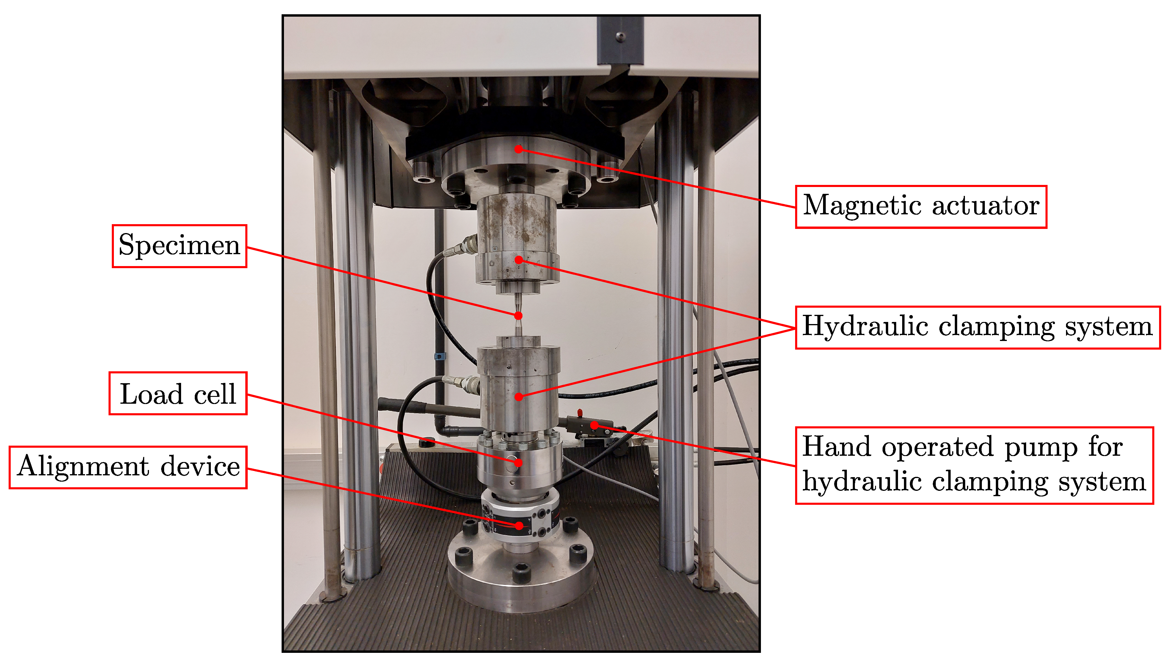
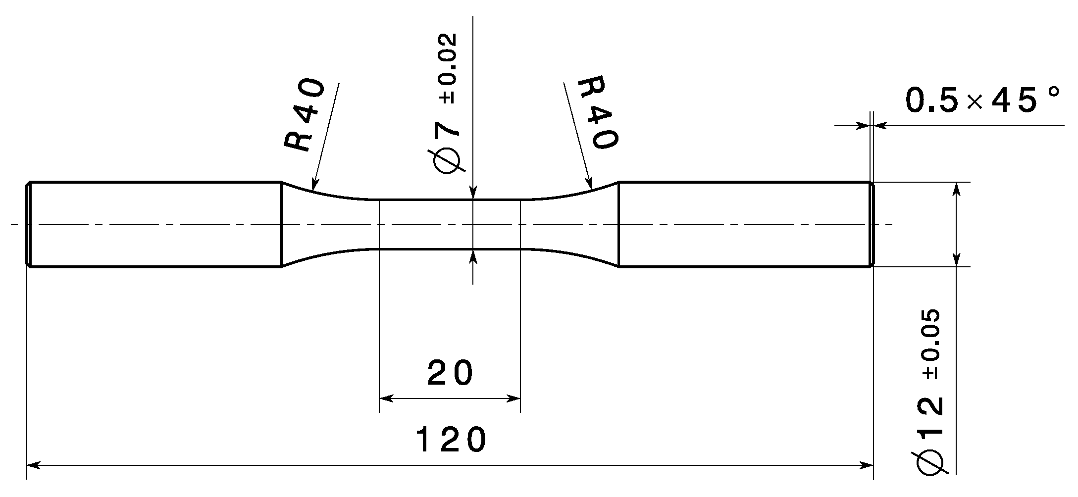
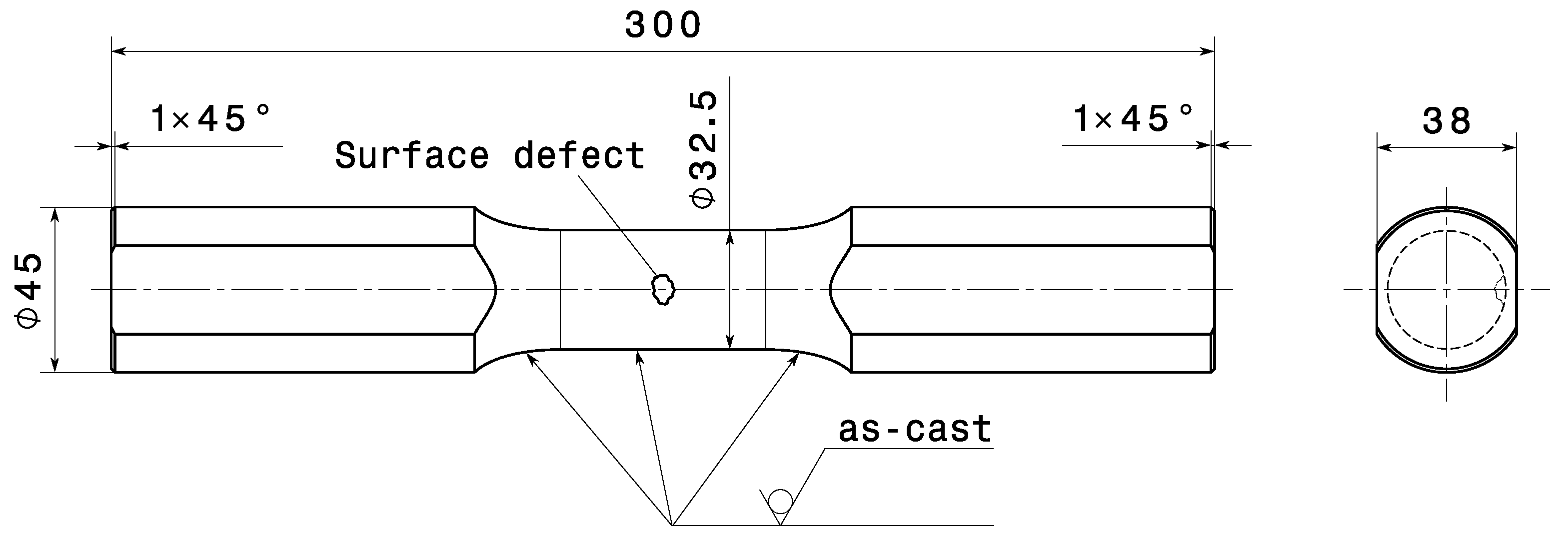
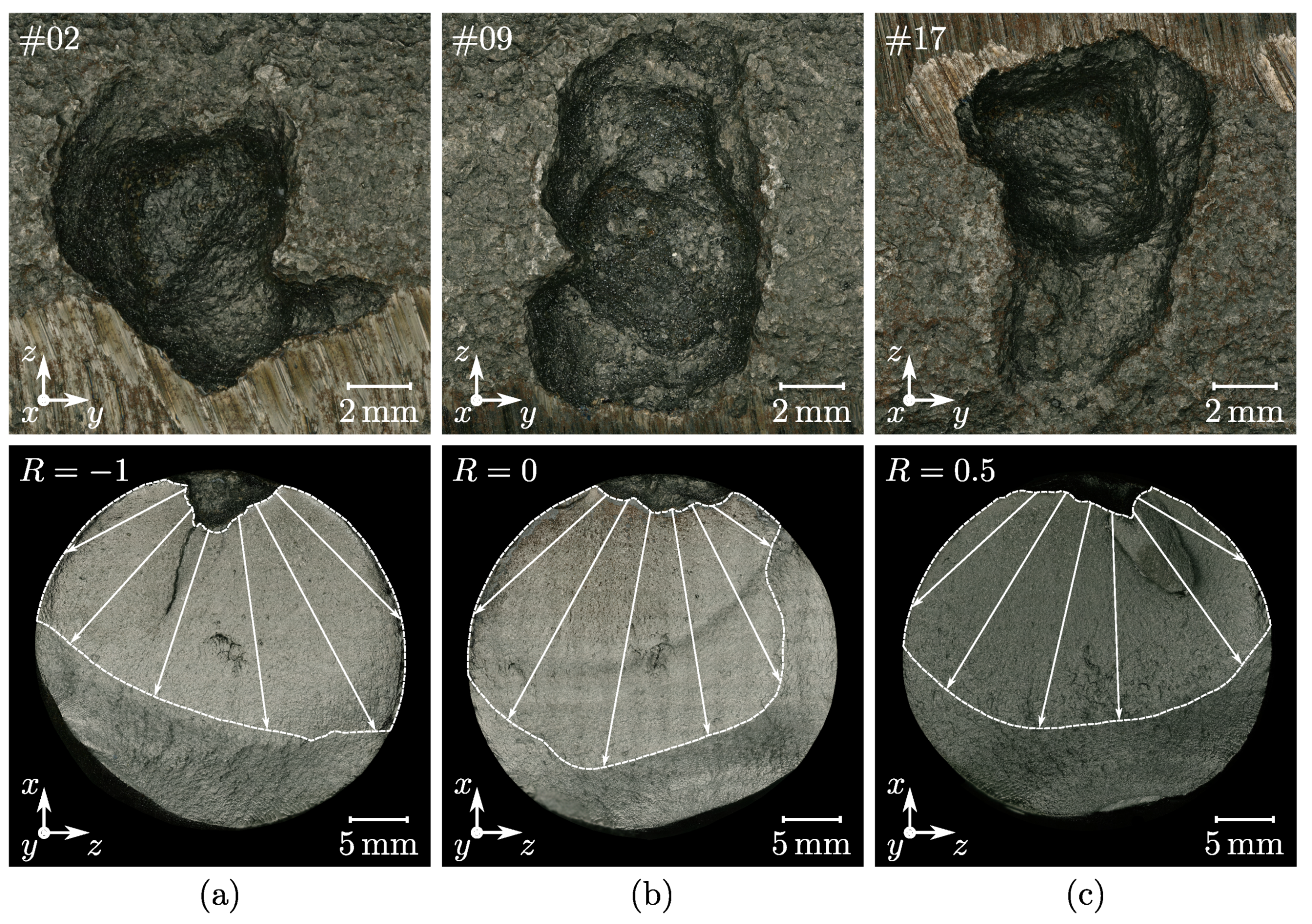
The low-cycle fatigue experiments reported in Section 2.1 are conducted utilizing the plain specimen geometry depicted in Figure 6. Hence, the description of the elastic–plastic strain as a function of stress according to Equation (4) is only valid for unnotched specimens, where the deformation behaviour is uniform in the loaded cross-section. As notched specimens exhibit a stress gradient emanating from the notch root, local plastic deformation can occur in the highly-stressed vicinity of the notch root, while elastic deformation is predominant in regions further away from it. Dealing with cyclic loading, this local plastic deformation results in effects such as mean stress relaxation in the notch vicinity, leading to a complex evolution of the acting stress field which cannot be described in an analytical manner. Thus, numerical analyses are necessary utilizing a proper material model capable of describing the inelastic material behaviour.

In the present study, a combined hardening model considering isotropic and non-linear kinematic hardening is chosen to describe the non-linear material behaviour. The model is based on the definition of a yield function f given in Equation (7) [30].

$$f=J\left(\sigma -\mathit{X}\right)-I-k$$

(7)

The term $J\left(\sigma -\mathit{X}\right)$ corresponds to the von Mises criterion and is defined by Equation (8) [30].

$$J\left(\sigma -\mathit{X}\right)=\sqrt{\frac{3}{2}\left({\sigma }^{\prime }-{\mathit{X}}^{\prime }\right):\left({\sigma }^{\prime }-{\mathit{X}}^{\prime }\right)}$$

(8)

Herein, the parameter $\sigma$ represents the stress tensor and $\mathit{X}$ corresponds to the kinematic back stress tensor. The parameters ${\sigma }^{\prime }$ and ${\mathit{X}}^{\prime }$ denote the deviatoric parts of $\sigma$ and $\mathit{X}$, respectively.

The yield function f reported in Equation (7) represents a surface in the space of stresses where plastic deformation of the stressed component takes place if the condition $f=0$ is fulfilled. In the case of $f<0$, the material flow is of a linear–elastic type. The initial size of f at zero plastic strain is described by the parameter k. During cyclic plastic loading, the dislocation structure inherent in the material is altered, resulting in a change of the size and the position of the yield surface f. The evolution of the surface size is described by the isotropic part I of the combined hardening approach according to Equation (9) [97].

$$I=Q·\left(1-e^{-b_{s}p}\right)$$

(9)

The size of the yield surface changes as a function of the accumulated plastic strain p, where the parameter Q denotes the difference between the initial and stabilized size of the yield surface and $b_s$ represents the stabilization rate under constant strain amplitude loading [28,30].

The position and translation of the yield surface in the space of stresses are governed by the kinematic part of the combined hardening model [97]. In order to improve the description accuracy of the non-linear material model, the kinematic back stress tensor $\mathit{X}$ is defined according to Equation (10) as a superposition of individual contributions ${\mathit{X}}_{\mathit{i}}$ [30].

$$\mathit{X}=\sum _{i=1}^n{\mathit{X}}_{\mathit{i}}$$

(10)

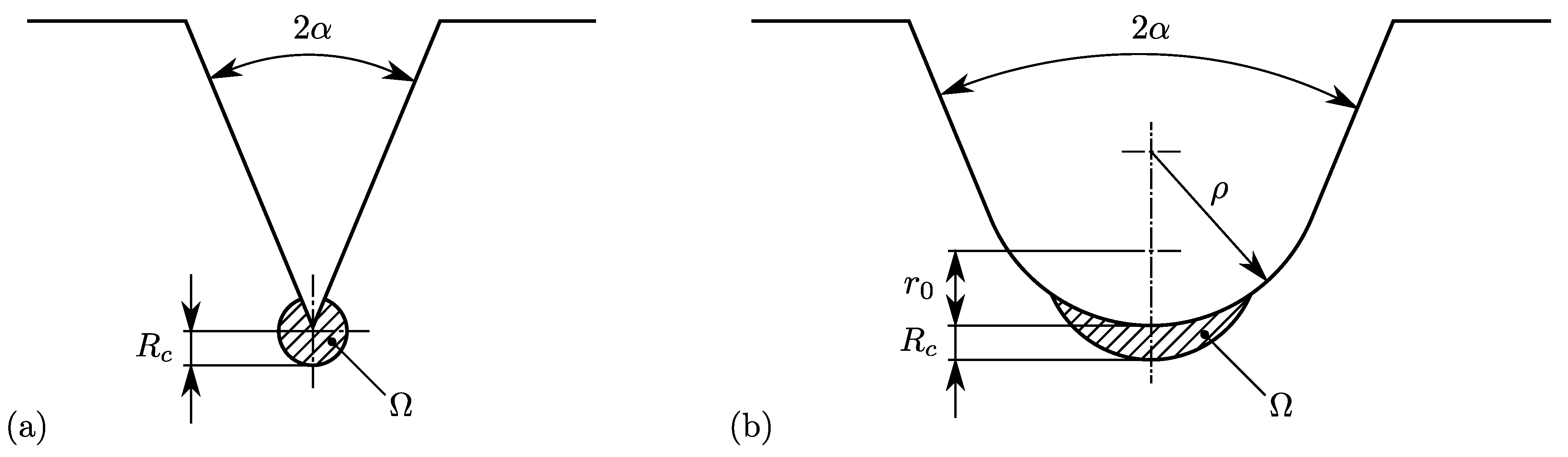
Each part ${\mathit{X}}_{\mathit{i}}$ follows a differential equation [98] which can be integrated to give Equation (11) for the uniaxial load case [28,30].

$$X_i=\psi \frac{C_i}{{\gamma }_i}+\left(X_{0,i}-\psi \frac{C_i}{{\gamma }_i}\right)·e^{-\psi {\gamma }_i\left[{\epsilon }^{\left(p\right)}-{\epsilon }_0^{\left(p\right)}\right]}$$

(11)

The parameters $X_{0,i}$ and ${\epsilon }_0^{\left(p\right)}$ represent the initial conditions, where ${\epsilon }^{\left(p\right)}$ denotes the plastic strain. The direction of the flow is described by $\psi$ which takes values of $\psi =\pm 1$.

In the present study, the parameters of the combined hardening model, including the kinematic material parameters $C_i$ and ${\gamma }_i$, as well as Q and $b_s$ of the isotropic part, are evaluated utilizing an optimization routine [31] which was developed at the Chair of Mechanical Engineering at the Montanuniversität Leoben. This routine was comprehensively validated for various materials under ambient and elevated temperatures [99,100,101,102,103]. In the present study, the material parameters featured in Equation (9) and (11) are determined based on the experimental data reported in Section 2.1. Concerning the non-linear kinematic part of the combined hardening model, two back stress components are considered.

Table 6. Parameters of the combined hardening material model.

$\mathit{k}$[MPa]	$\mathit{Q}$[MPa]	${\mathit{b}}_{\mathit{S}}[-]$	${\mathit{C}}_1$[MPa]	${\mathit{\gamma }}_1$$[-]$	${\mathit{C}}_2$[MPa]	${\mathit{\gamma }}_2[-]$
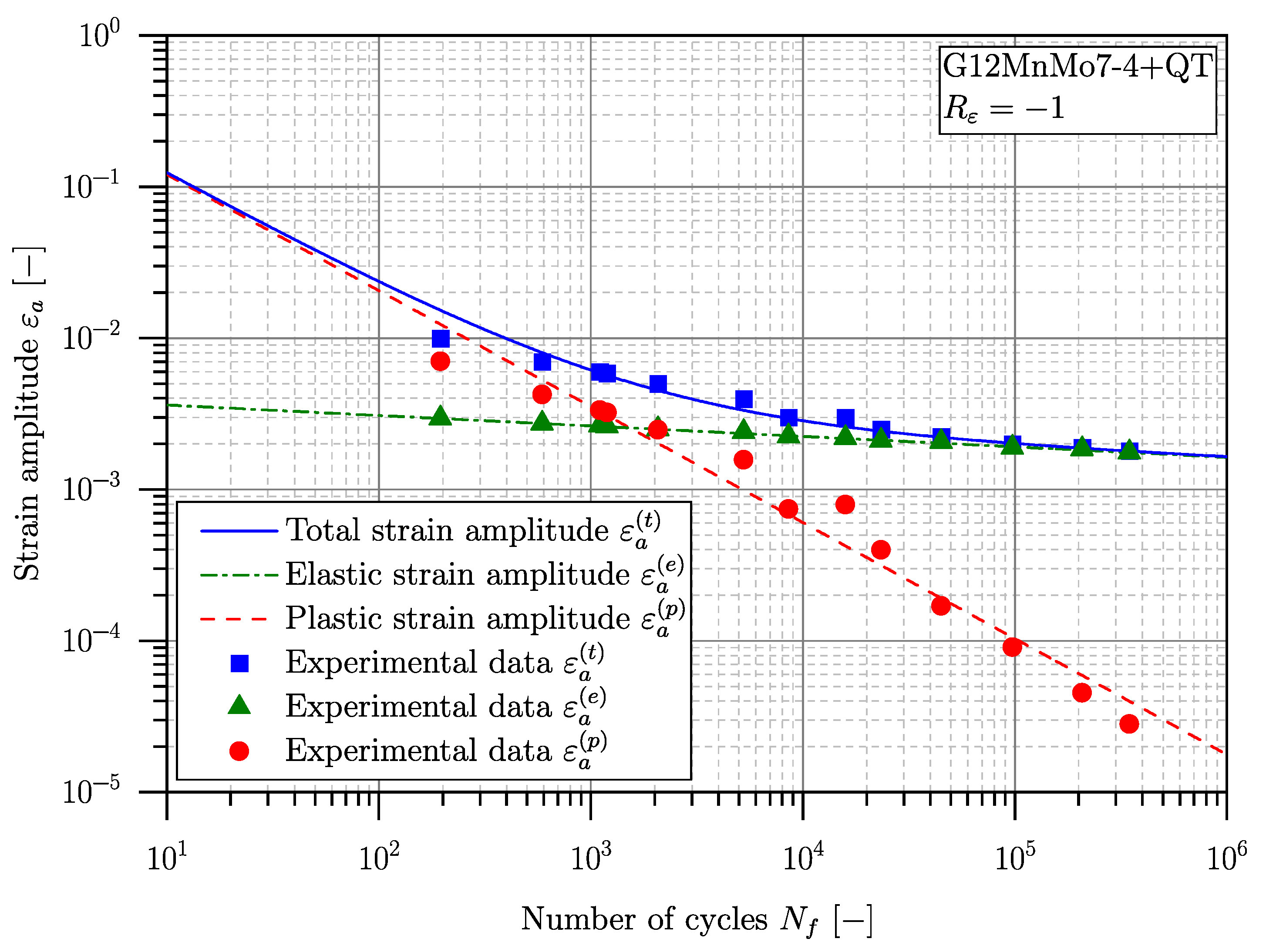
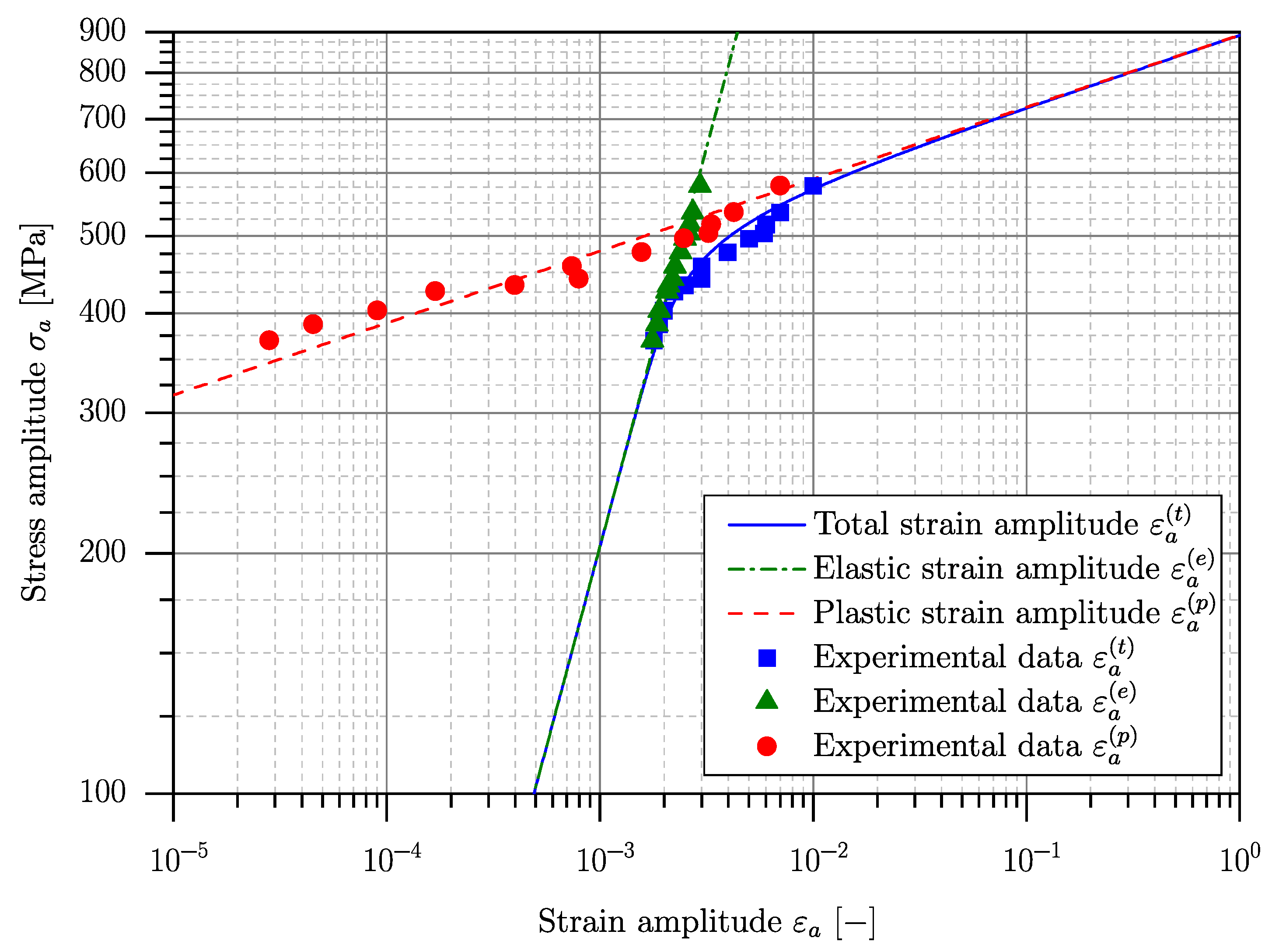
470	$-290.5$	150.2	899,436	8996	133,620	522.7

summarizes the parameters of the elastic–plastic material model.

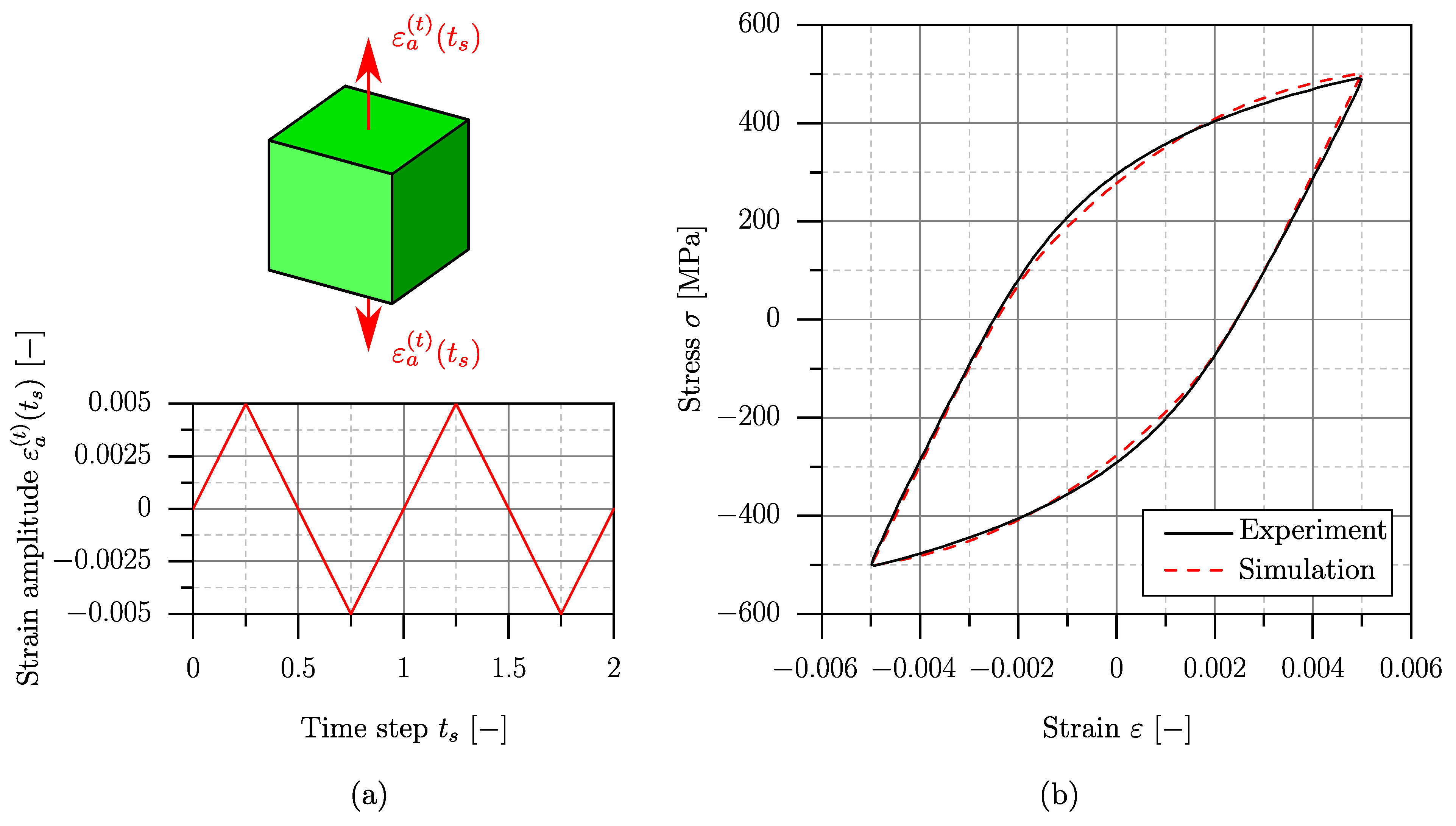
As the material parameters are determined, validation of the constitutional model is carried out by a non-linear finite element analysis in Abaqus^® 2021. A single three-dimensional element of unity edge length is utilised to evaluate the stabilized hysteresis loop at a total strain amplitude of ${\epsilon }_a^{\left(t\right)}=0.5\%$. The element is of the type C3D20 and features quadratic shape functions. Figure 16 depicts the finite element model, as well as the numerically evaluated hysteresis loop for the stabilized material condition in contrast to the experimental results. In this case, a stabilization of the hysteresis loop has been obtained after approximately 1100 cycles.

The comparison of numerical and experimental results given in Figure 16 reveals a satisfying representation of the stabilized cyclic material behaviour by the established combined hardening model.

3.3. Evaluation of the Elastic–Plastic Design Limit Curve

As the non-linear material behaviour of the investigated cast steel alloy G12MnMo7-4+QT is characterized, the elastic–plastic design limit curve can be assessed by means of an energy-based approach. This limit curve is further utilised to calculate the fatigue strength of defect-afflicted components. In order to derive the elastic–plastic design limit curve, the experimental high-cycle fatigue results of small-scale specimens, reported in a preceding study [10], are reassessed.

The elastic–plastic design limit curve is evaluated based on the averaged total strain energy density $\Delta {\overline{W}}^{\left(t\right)}$. Therefore, finite element analyses are conducted utilizing Abaqus^® 2021. The non-linear material behaviour is considered by implementation of the combined hardening model presented in Section 3.2. Axisymmetric models are utilised to evaluate $\Delta {\overline{W}}^{\left(t\right)}$ of the respective plain and notched specimens, featuring elements of type CAX6/CAX8 with quadratic shape functions. The control volume is modelled by partitioning of the notched geometries, considering a control radius of $R_c=0.083$ mm, as evaluated in [10] for G12MnMo7-4+QT. Herein, the evaluation of $R_c$ was conducted following the linear–elastic framework given in [40,41], considering the fatigue strength and long-crack growth threshold stress intensity factor range which correspond to the fatigue limit at ten million load cycles. Three different stress ratios R have been observed, where $R_c$ is defined as the arithmetic mean value. In order to ensure appropriate element sizing within the control volume $\mathsf{\Omega }$, the results of a mesh sensitivity study conducted in a preceding study [104] are considered. The SED within $\mathsf{\Omega }$ is rather insensitive to the element size. Hence, control volumes consisting of a minimum of three elements yield appropriate SED values without sacrificing accuracy, as also stated in [105]. The position $r_0$ of the control volume center point is derived according to [42] for the investigated notch opening angles of $2\alpha ={45}^{\circ }$ and $2\alpha ={135}^{\circ }$. The numerical models are stressed under uniaxial tension-compression loading, covering the tested load amplitudes and stress ratios of the high-cycle fatigue experiments conducted in [10]. A cyclic load is applied during numerical analysis until stabilization of the material behaviour is achieved. Stabilization is assumed if the iterative change in stresses of each cycle is less than approximately one percent. This was obtained after approximately one hundred load cycles for the conducted simulations. The cyclic load in Abaqus^® 2021 is realized by the definition of a time-dependent multiplier $m_R$, altering the currently acting load which corresponds to the investigated stress range $\Delta \sigma$. Figure 17 exemplarily depicts the finite element model of the investigated V-notched specimen geometry possessing a notch opening angle of $2\alpha ={45}^{\circ }$. The presented stress result refers to the stabilized material condition at a stress range of $\Delta \sigma =120$ MPa and a stress ratio of $R=-1$. The specimen is depicted for the maximum value of the numerical cyclic load. Furthermore, the course of the load multiplier $m_R$ utilised for the cyclic simulations is depicted for all investigated load ratios for the first two cycles.

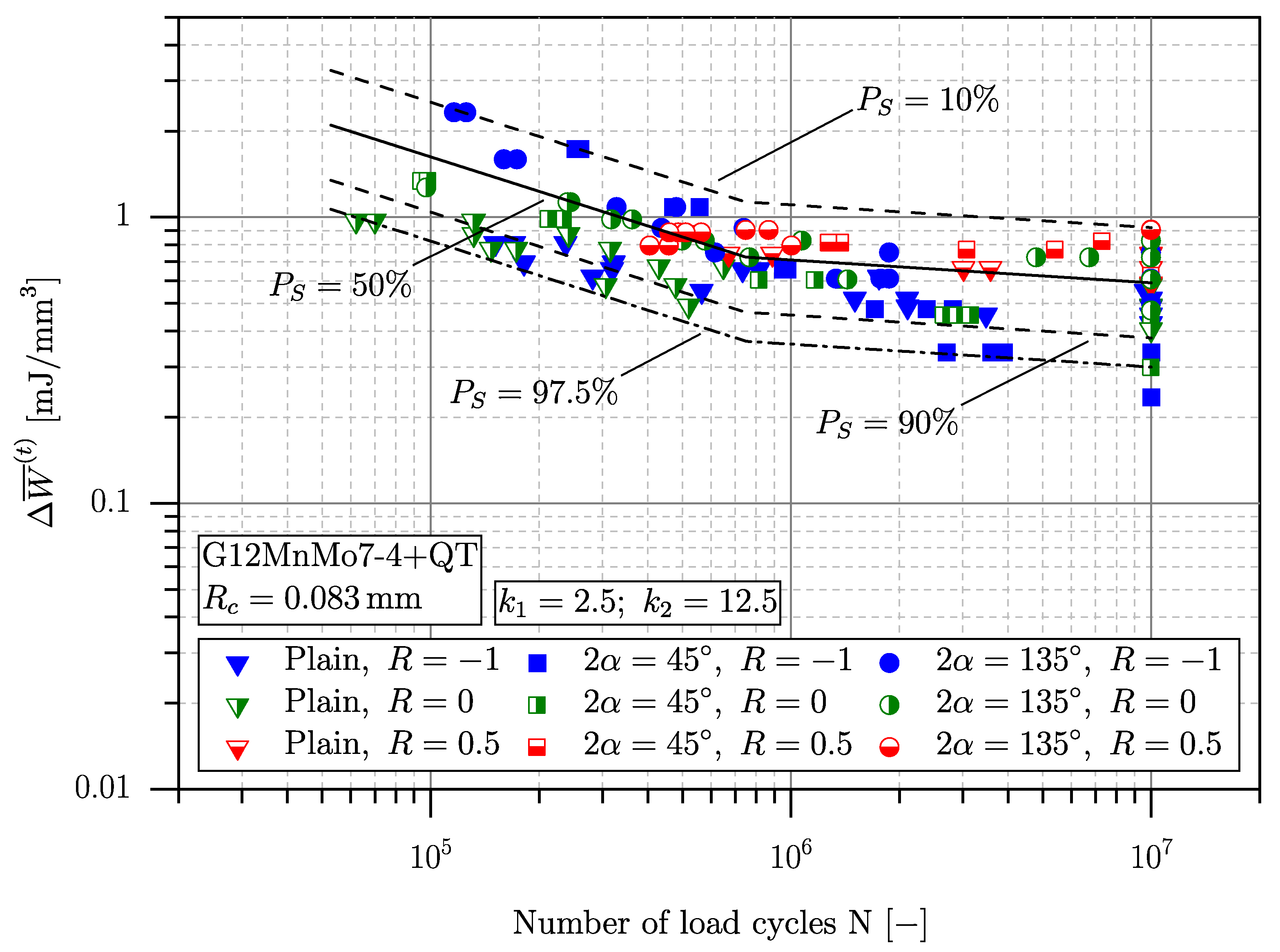
Finally, the elastic and plastic strain energy contributions are evaluated from the control volume elements and the averaged total strain energy density in the stabilized material condition is calculated. Figure 18 summarizes the elastic–plastic fatigue assessment results.

Concerning the long-life fatigue strength, the presented results are statistically evaluated according to the $arcsin\sqrt{P}$ approach [106]. The finite-life fatigue regime is assessed following ASTM E739 [107], including the statistical evaluation of the fatigue limit curves for a probability of survival of $P_S=50\%$, as well as for values of $P_S=10\%$ and $P_S=90\%$. Furthermore, the limit curve for $P_S=97.5\%$ is depicted, which serves as an assessment basis in fatigue design, according to the widely used guideline FKM (Forschungskuratorium Maschinenbau) [18].

As depicted in Figure 18, the elastic–plastic fatigue assessment based on the total strain energy density summarizes the fatigue results of three different specimen geometries tested at three different stress ratios into a unique narrow scatter band. The scatter index which is defined by the limit curves of $P_S=10\%$ and $P_S=90\%$ possesses a value of $1:T_{\Delta {\overline{W}}^{\left(t\right)}}=2.43$. Comparing to the scatter index of $1:T_{\Delta {\overline{W}}^{\left(e\right)}}=4.32$ as reported in [10] utilizing a linear–elastic SED approach, the consideration of the non-linear material behaviour by the total SED provides a significant improvement in prediction accuracy. As stated in [10], the comparably high value of $1:T_{\Delta {\overline{W}}^{\left(e\right)}}$ is primarily assigned to the assessment results at a stress ratio of $R=0.5$. Due to the high maximum loads, inelastic material deformation and related mean stress relaxation occur, which cannot be considered by the linear–elastic framework. This leads to an overestimation of the local inherent deformation energy and therefore an increased scatter index when gathering the fatigue assessment results obtained at different stress ratios. The overestimation due to the linear–elastic formulation holds especially true when dealing with high provoked stress concentrations, as in the case of sharply notched components. 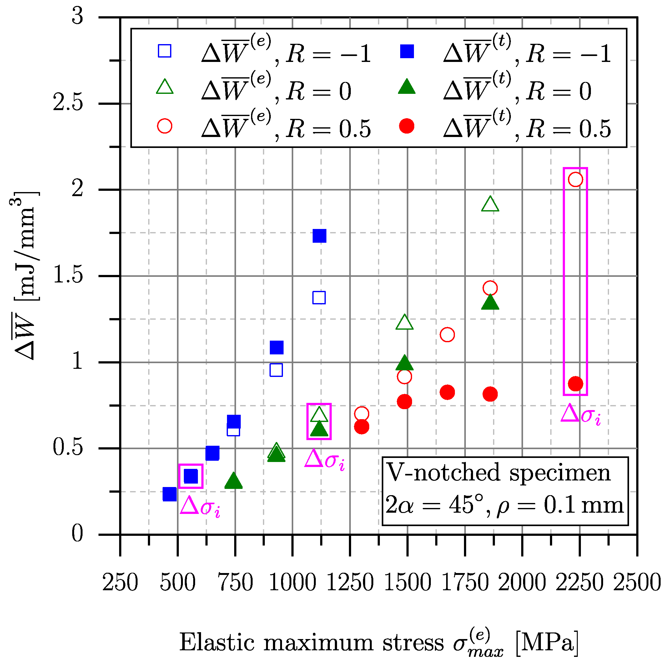To illustrate the localized plastic deformation effect and its associated mean stress relaxation, a comparison between the results of the linear–elastic and the elastic–plastic SED concept is presented in Figure 19. Both concepts are utilised to assess V-notched specimens with a notch opening angle of $2\alpha ={45}^{\circ }$ and a notch root radius of $\rho =0.1$ mm. The linear–elastic SED $\Delta {\overline{W}}^{\left(e\right)}$ is calculated analytically utilizing the framework given in [42]. To consider the stress ratio in the calculation of $\Delta {\overline{W}}^{\left(e\right)}$, the correction factor $c_w$ according to [61] is implemented. The total SED $\Delta {\overline{W}}^{\left(t\right)}$ is evaluated numerically utilizing the set up combined hardening model. The derived SED values are depicted over the linear–elastic maximum stress as a reference.

Reflecting the data points given in Figure 19, the effect of cyclic mean stress relaxation can be observed. As the theoretical linear–elastic maximum stress increases, the total SED and the purely linear–elastic SED diverge from each other due to occurring plastic deformation in the vicinity of the notch root. In order to describe the effect of stress ratio, the behaviour of a common load level $\Delta {\sigma }_i$ is studied first. These calculations are highlighted by an additional bounding box in Figure 19. $\Delta {\sigma }_i$ is chosen such that the deformation is mainly linear–elastic in the case of $R=-1$. Hence, there is no significant difference between $\Delta {\overline{W}}^{\left(e\right)}$ and $\Delta {\overline{W}}^{\left(t\right)}$. As the stress ratio and therefore the maximum stress increases, the mismatch between the elastic–plastic and the purely linear–elastic solution becomes more pronounced. This behaviour is explained by the occurring mean stress relaxation due to plastic deformation and the associated decrease in the locally acting stress ratio.

Second, the combined effect of stress range and stress ratio is investigated. Examining the depicted results in Figure 19, one can observe opposite trends of $\Delta {\overline{W}}^{\left(t\right)}$ compared to $\Delta {\overline{W}}^{\left(e\right)}$ as the stress range and stress ratio increase; while $\Delta {\overline{W}}^{\left(t\right)}$ takes higher values than $\Delta {\overline{W}}^{\left(e\right)}$ with an increasing stress range in the case of $R=-1$, the calculated results of $\Delta {\overline{W}}^{\left(t\right)}$ decrease compared to $\Delta {\overline{W}}^{\left(e\right)}$ in the case of higher stress ratios. This is reasoned by the cyclic plastic deformation which contributes a significant amount to the total SED in the case of $R=-1$. Considering $R=0$ and $R=0.5$, the bearable stress ranges are relatively small compared to $R=-1$, resulting in a mainly elastic cyclic deformation. Hence, the contribution of the cyclic plastic SED to $\Delta {\overline{W}}^{\left(t\right)}$ cannot compensate for the dominant reduction of the cyclic elastic SED term due to mean stress relaxation. This results in an overall decrease of $\Delta {\overline{W}}^{\left(t\right)}$ compared to $\Delta {\overline{W}}^{\left(e\right)}$.

As demonstrated, the implementation of the non-linear material behaviour severely affects the local stress field and therefore the fatigue behaviour of cast steel components. However, the elastic–plastic finite element analyses necessary to evaluate the total strain energy density increase computational efforts significantly. In order to keep time and cost expenses at a minimum, an alternative evaluation methodology based on the acting linear–elastic stress and strain field is studied next.

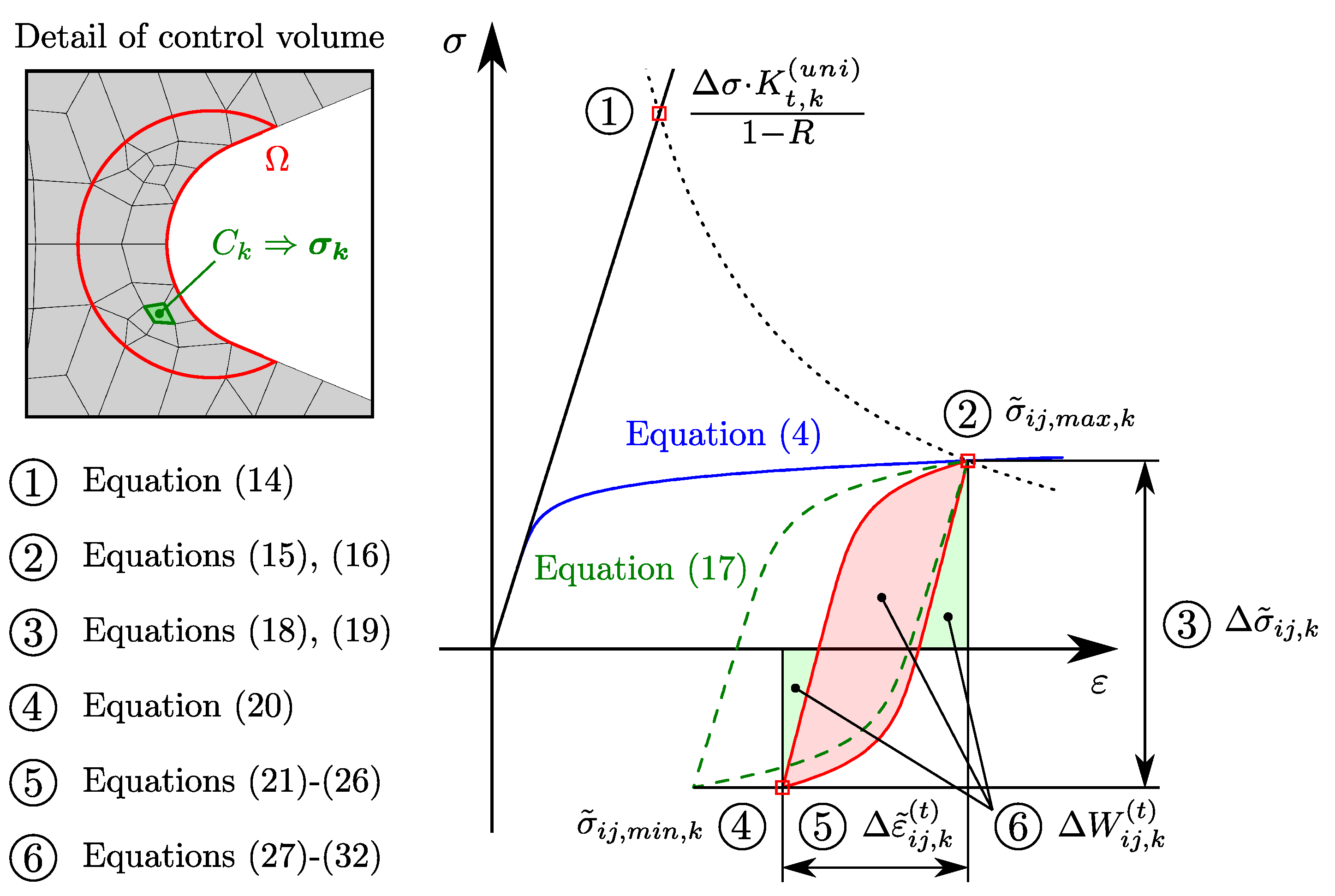
3.4. A Numerically Efficient Approximation Approach to Evaluate the Elastic–Plastic Strain Energy Density

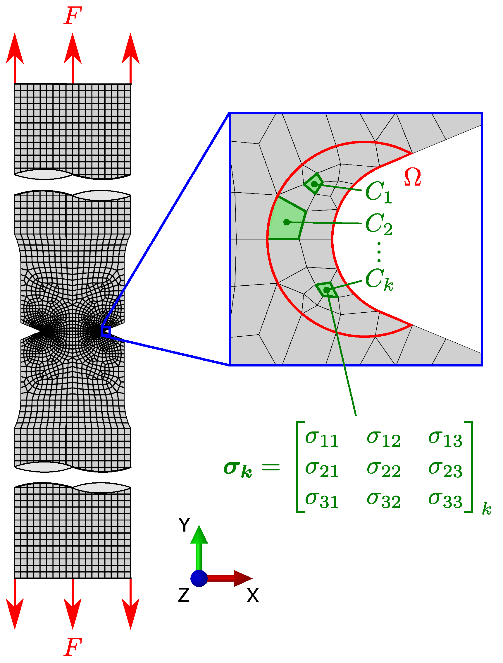
In order to derive an engineering-feasible methodology for the approximation of the averaged elastic–plastic strain energy density $\Delta {\overline{W}}^{\left(t\right)}$ at complexly shaped casting imperfections, the V-notched specimens are investigated firstly. The respective specimen geometries correspond to the ones utilised for evaluation of the elastic–plastic design limit curve presented in Section 3.3. As $\Delta {\overline{W}}^{\left(t\right)}$ is defined by the stabilized hysteresis loop, see Figure 2, the non-linear stress and strain fields have to be calculated within the finite control volume $\mathsf{\Omega }$ in order to derive $\Delta {\overline{W}}^{\left(t\right)}$. Due to the general multiaxiality of the local acting stress state, the presented methodology is formulated to include all components of the stress tensor $\sigma$ and strain tensor $\epsilon$ given in Equations (12) and (13).

$$\sigma =\left[\begin{array}{ccc}{\sigma }_{11}& {\sigma }_{12}& {\sigma }_{13}\\ {\sigma }_{21}& {\sigma }_{22}& {\sigma }_{23}\\ {\sigma }_{31}& {\sigma }_{32}& {\sigma }_{33}\end{array}\right]$$

(12)

$$\epsilon =\left[\begin{array}{ccc}{\epsilon }_{11}& {\epsilon }_{12}& {\epsilon }_{13}\\ {\epsilon }_{21}& {\epsilon }_{22}& {\epsilon }_{23}\\ {\epsilon }_{31}& {\epsilon }_{32}& {\epsilon }_{33}\end{array}\right]$$

(13)

In the following, the components of $\sigma$ and $\epsilon$ are denoted as ${\sigma }_{ij}$ and ${\epsilon }_{ij}$, where $i,j\in \{1,2,3\}$. For the sake of completeness, it should be noted that ${\sigma }_{ij}={\sigma }_{ji}$ and ${\epsilon }_{ij}={\epsilon }_{ji}$, due to the symmetry of $\sigma$ and $\epsilon$.

The definition of the applied approximation method for a component loaded under an arbitrary stress range $\Delta \sigma$ and a stress ratio of R is demonstrated for V-notched specimens, possessing a notch opening angle of $2\alpha ={45}^{\circ }$ and a notch root radius of $\rho =0.1$ mm. In the present study, the conservative concept according to Neuber [69] is chosen to evaluate the elastic–plastic stresses and strains in the control volume $\mathsf{\Omega }$. This necessitates the evaluation of the linear–elastic stress tensor ${\sigma }_{\mathit{k}}$ for each finite element $C_k$ within $\mathsf{\Omega }$. Therefore, a linear–elastic finite element analysis is carried out, utilizing a stress of 1 MPa in the cross-section with a diameter of 16 mm. Figure 20 schematically depicts the numerical model and the control volume of the investigated V-notched specimen geometry.

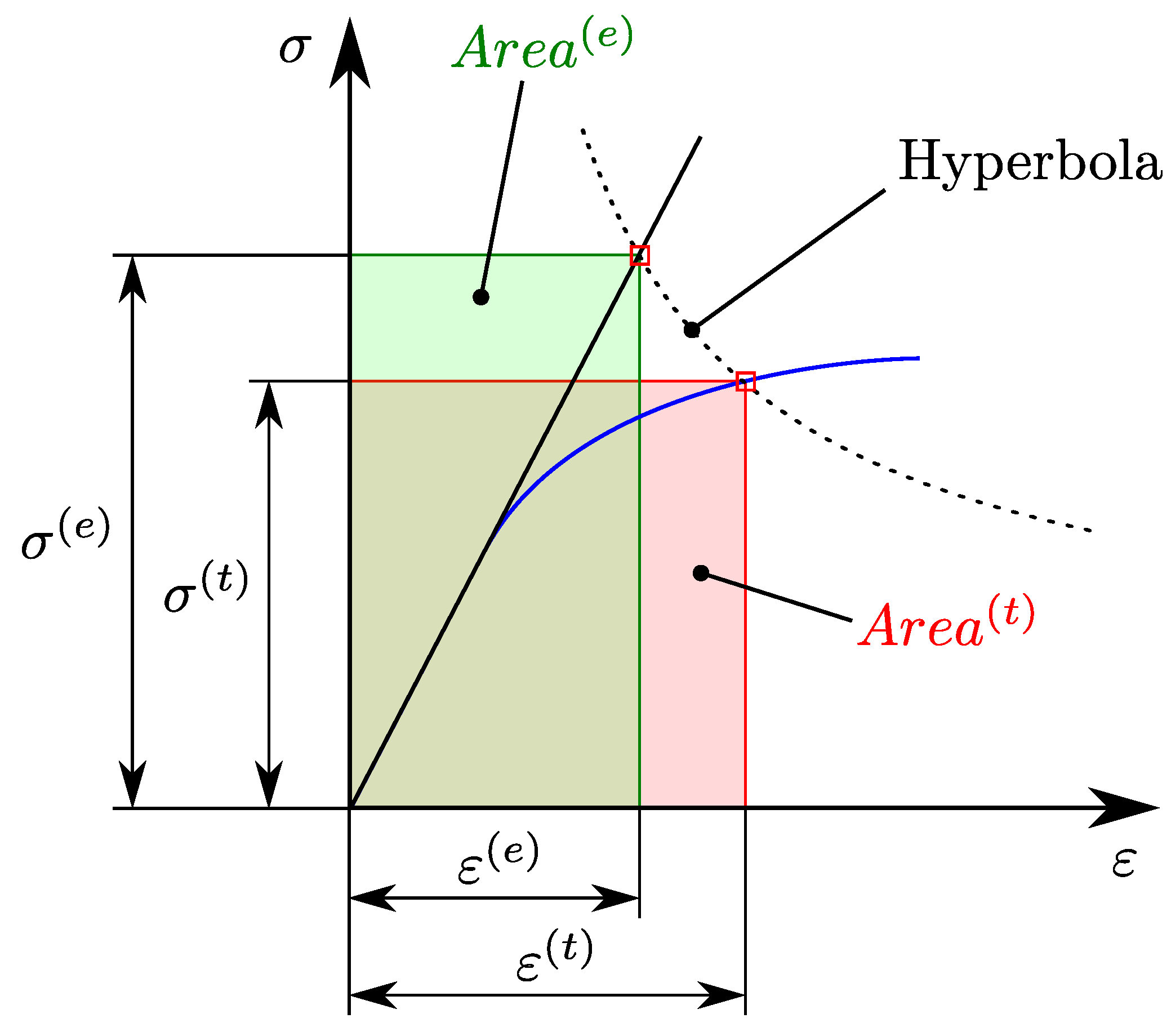
The stress components ${\sigma }_{ij,k}$ are evaluated in the centroid of the respective element $C_k$. Due to the utilization of a stress of 1 MPa in the specimen cross-section, ${\sigma }_{ij,k}$ constitutes the elemental stress concentration factors for the individual directions in the space of stresses. In order to approximate the elastic–plastic stresses and strains for cyclic loading of the specimen, the cyclic stress–strain curve, as evaluated in Section 3.1, is utilised with some additional considerations. The low-cycle fatigue experiments conducted to determine the cyclic stress–strain curve utilised plain specimens loaded under uniaxial tension-compression loading. This implies the existence of a uniaxial stress state in the specimen cross-section. Hence, the cyclic stress–strain curve described by Equation (4) is only valid for a uniaxial stress state. As the evaluated stress tensor of element $C_k$ possesses in general more than one non-zero component, an equivalent stress has to be calculated in order to apply Neuber’s approximation concept. Therefore, the von Mises yield criterion [108] is applied, which is based on the second invariant $J_2$ of the deviatoric part of the stress tensor ${\sigma }_{\mathit{k}}$. The derived equivalent stress represents the stress concentration factor $K_{t,k}^{\left(uni\right)}$, which is calculated according to Equation (14). The superscript $\left(uni\right)$ denotes that the respective parameter is evaluated for the equivalent uniaxial stress state.

$$K_{t,k}^{\left(uni\right)}=\sqrt{3·J_2}=\sqrt{\frac{1}{2}\left[{\left({\sigma }_{11,k}-{\sigma }_{22,k}\right)}^2+{\left({\sigma }_{22,k}-{\sigma }_{33,k}\right)}^2+{\left({\sigma }_{33,k}-{\sigma }_{11,k}\right)}^2+6\left({\sigma }_{23,k}^2+{\sigma }_{31,k}^2+{\sigma }_{12,k}^2\right)\right]}$$

(14)

Utilizing $K_{t,k}^{\left(uni\right)}$ and the cyclic stress–strain curve given by Equation (4), the elastic–plastic stresses and strains within $C_k$ can be approximated. At first, the uniaxial maximum stress ${\tilde{\sigma }}_{max,k}^{\left(uni\right)}$ during cyclic loading is calculated by minimizing the objective function given in Equation (15). The tilde accent denotes elastic–plastic parameters evaluated by the approximation framework.

$$\frac{1}{E^{\prime }}{\left[{\tilde{\sigma }}_{max,k}^{\left(uni\right)}\right]}^2+{\tilde{\sigma }}_{max,k}^{\left(uni\right)}{\left[\frac{{\tilde{\sigma }}_{max,k}^{\left(uni\right)}}{K^{\prime }}\right]}^{\frac{1}{n^{\prime }}}-\frac{1}{E^{\prime }}{\left[\frac{\Delta \sigma ·K_{t,k}^{\left(uni\right)}}{1-R}\right]}^2=0$$

(15)

To derive the maximum stress values of the components of the elastic–plastic stress tensor ${\tilde{\sigma }}_{\mathit{k}}$ from the approximated uniaxial maximum stress ${\tilde{\sigma }}_{max,k}^{\left(uni\right)}$, an additional assumption has to be made. Hereby, the ratio between the linear–elastic components ${\sigma }_{ij,k}$ and the equivalent stress $K_{t,k}^{\left(uni\right)}$ is studied and it is assumed that this ratio remains valid in the case of non-linear material behaviour. Thus, the elastic–plastic maximum values ${\tilde{\sigma }}_{ij,max,k}$ of the components of ${\tilde{\sigma }}_{\mathit{k}}$ can be computed according to Equation (16).

$${\tilde{\sigma }}_{ij,max,k}={\sigma }_{ij,k}·\frac{{\tilde{\sigma }}_{max,k}^{\left(uni\right)}}{K_{t,k}^{\left(uni\right)}}$$

(16)

The values of ${\tilde{\sigma }}_{ij,max,k}$ constitute the upper reversal points of the approximated hysteresis loops during cyclic loading. In order to define also the lower reversal points, the elastic–plastic stress ranges $\Delta {\tilde{\sigma }}_{ij,k}$ have to be calculated. As the investigated cast steel alloy G12MnMo7-4+QT exhibits Masing behaviour [109], the cyclic strains can be described as a function of the stress ranges according to Equation (17).

$$\Delta {\epsilon }^{\left(t\right)}=\Delta {\epsilon }^{\left(e\right)}+\Delta {\epsilon }^{\left(p\right)}=\frac{\Delta \sigma }{E^{\prime }}+2{\left(\frac{\Delta \sigma }{2·K^{\prime }}\right)}^{\frac{1}{n^{\prime }}}$$

(17)

It should be noted that Equation (17) results from Equation (4) by substituting the amplitude terms for half of the respective ranges, for example, ${\sigma }_a=\Delta \sigma /2$. Thus, Equation (17) is also only valid for the uniaxial stress state. Utilizing $K_{t,k}^{\left(uni\right)}$, the equivalent uniaxial stress range $\Delta {\tilde{\sigma }}_k^{\left(uni\right)}$ of the finite element $C_k$ within $\mathsf{\Omega }$ is calculated by minimizing the objective function given in Equation (18).

$$\frac{1}{E^{\prime }}{\left[\Delta {\tilde{\sigma }}_k^{\left(uni\right)}\right]}^2+2·\Delta {\tilde{\sigma }}_k^{\left(uni\right)}{\left[\frac{\Delta {\tilde{\sigma }}_k^{\left(uni\right)}}{2·K^{\prime }}\right]}^{\frac{1}{n^{\prime }}}-\frac{1}{E^{\prime }}{\left[\Delta \sigma ·K_{t,k}^{\left(uni\right)}\right]}^2=0$$

(18)

In order to evaluate the elastic–plastic stress ranges $\Delta {\tilde{\sigma }}_{ij,k}$, the relationship reported in Equation (16) is utilised in terms of cyclic stresses according to Equation (19).

$$\Delta {\tilde{\sigma }}_{ij,k}={\sigma }_{ij,k}·\frac{\Delta {\tilde{\sigma }}_k^{\left(uni\right)}}{K_{t,k}^{\left(uni\right)}}$$

(19)

Subsequently, the minimum stresses ${\tilde{\sigma }}_{ij,min,k}$ can be calculated following Equation (20), constituting the lower reversal points of the approximated cyclic hysteresis loops.

$${\tilde{\sigma }}_{ij,min,k}={\tilde{\sigma }}_{ij,max,k}-\Delta {\tilde{\sigma }}_{ij,k}$$

(20)

As the cyclic hysteresis loops in element $C_k$ are characterized in terms of the acting stress components, the corresponding strain components of the elastic–plastic strain tensor ${\tilde{\epsilon }}_{\mathit{k}}$ have to be evaluated. Utilizing Hooke’s law, the elastic strain ranges are computed according to Equation (21), where $\nu$ represents Poisson’s ratio and ${\delta }_{ij}$ represents the Kronecker delta.

$$\Delta {\tilde{\epsilon }}_{ij,k}^{\left(e\right)}=\frac{1+\nu }{E^{\prime }}\Delta {\tilde{\sigma }}_{ij,k}-\frac{\nu }{E^{\prime }}\left(\Delta {\tilde{\sigma }}_{11,k}+\Delta {\tilde{\sigma }}_{22,k}+\Delta {\tilde{\sigma }}_{33,k}\right){\delta }_{ij}$$

(21)

While the elastic strain components in the multiaxial stress state can be analytically evaluated following Equation (21), the calculation of the plastic strain contributions $\Delta {\tilde{\epsilon }}_{ij,k}^{\left(p\right)}$ needs some further consideration. The evaluation of the plastic strain ranges following Equation (17) is only valid for the uniaxial stress state, as the underlying experiments were conducted utilizing plain specimens subjected to uniaxial tension-compression loading. Hence, a direct calculation of the individual components $\Delta {\tilde{\epsilon }}_{ij,k}^{\left(p\right)}$ of ${\tilde{\epsilon }}_{\mathit{k}}$ utilizing Equation (17) is impermissible. Similar to Equations (16) and (19), an assumption based on the behaviour in the uniaxial stress state has to be made to approximate the plastic contributions $\Delta {\tilde{\epsilon }}_{ij,k}^{\left(p\right)}$. Therefore, the ratio between the plastic and elastic strain for the equivalent stress $\Delta {\tilde{\sigma }}_k^{\left(uni\right)}$ is calculated based on Equation (17) and it is assumed that this ratio is valid also in the case of a multiaxial stress state. Hence, the plastic strain ranges $\Delta {\tilde{\epsilon }}_{ij,k}^{\left(p\right)}$ are approximated according to Equation (22).

$$\Delta {\tilde{\epsilon }}_{ij,k}^{\left(p\right)}=\Delta {\tilde{\epsilon }}_{ij,k}^{\left(e\right)}·E^{\prime }·{\left(\frac{2^{n^{\prime }-1}}{K^{\prime }}\right)}^{\frac{1}{n^{\prime }}}·{\left[\Delta {\tilde{\sigma }}_k^{\left(uni\right)}\right]}^{\frac{1-n^{\prime }}{n^{\prime }}}$$

(22)

Finally, the total strain ranges $\Delta {\tilde{\epsilon }}_{ij,k}^{\left(t\right)}$ are calculated as a superposition of the elastic and plastic contributions, as given in Equation (23).

$$\Delta {\tilde{\epsilon }}_{ij,k}^{\left(t\right)}=\Delta {\tilde{\epsilon }}_{ij,k}^{\left(e\right)}+\Delta {\tilde{\epsilon }}_{ij,k}^{\left(p\right)}$$

(23)

As the stress and strain parameters describing the elastic–plastic hysteresis loops during cyclic loading are evaluated for the elements within the control volume $\mathsf{\Omega }$, the total averaged strain energy density $\Delta {\overline{W}}^{\left(t\right)}$ is calculated. The evaluation is carried out for each component of ${\tilde{\sigma }}_{\mathit{k}}$. After computation of the individual contributions, a superposition is carried out to derive $\Delta {\overline{W}}^{\left(t\right)}$. The general evaluation procedure is exemplified for element $C_k$ within $\mathsf{\Omega }$.

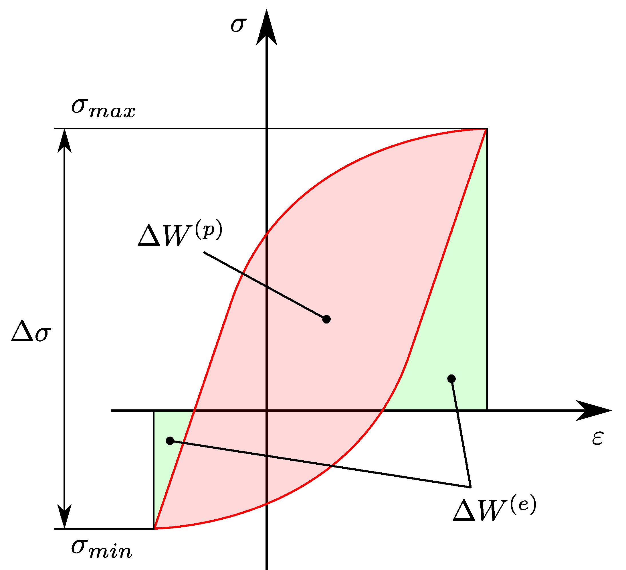
As illustrated in Figure 2, the cyclic stabilized hysteresis loop defines the elastic and plastic SED during cyclic loading. Hence, the respective contributions to the total SED can be evaluated simply by calculating the corresponding areas in the stress–strain diagram. In the uniaxial load case, the ascending and descending branches of the hysteresis loop are described by Equation (17). When dealing with a local multiaxial stress state, simply inserting the stress range component $\Delta {\tilde{\sigma }}_{ij,k}$ into Equation (17) will therefore not result in the calculated total strain range $\Delta {\tilde{\epsilon }}_{ij,k}^{\left(t\right)}$. In order to derive a valid description of $\Delta {\tilde{\epsilon }}_{ij,k}^{\left(t\right)}$ when dealing with individual stress components $\Delta {\tilde{\sigma }}_{ij,k}$, some other considerations have to be made. Stress and strain in a specific volume element are connected through the stiffness of the respective body. Hence, modulation of the stiffness leads to a change in strain when the acting stress parameter is kept constant. In terms of cyclic loading, the stiffness in the stress–strain relationship according to Equation (17) is described by $E^{\prime }$ and $K^{\prime }$. 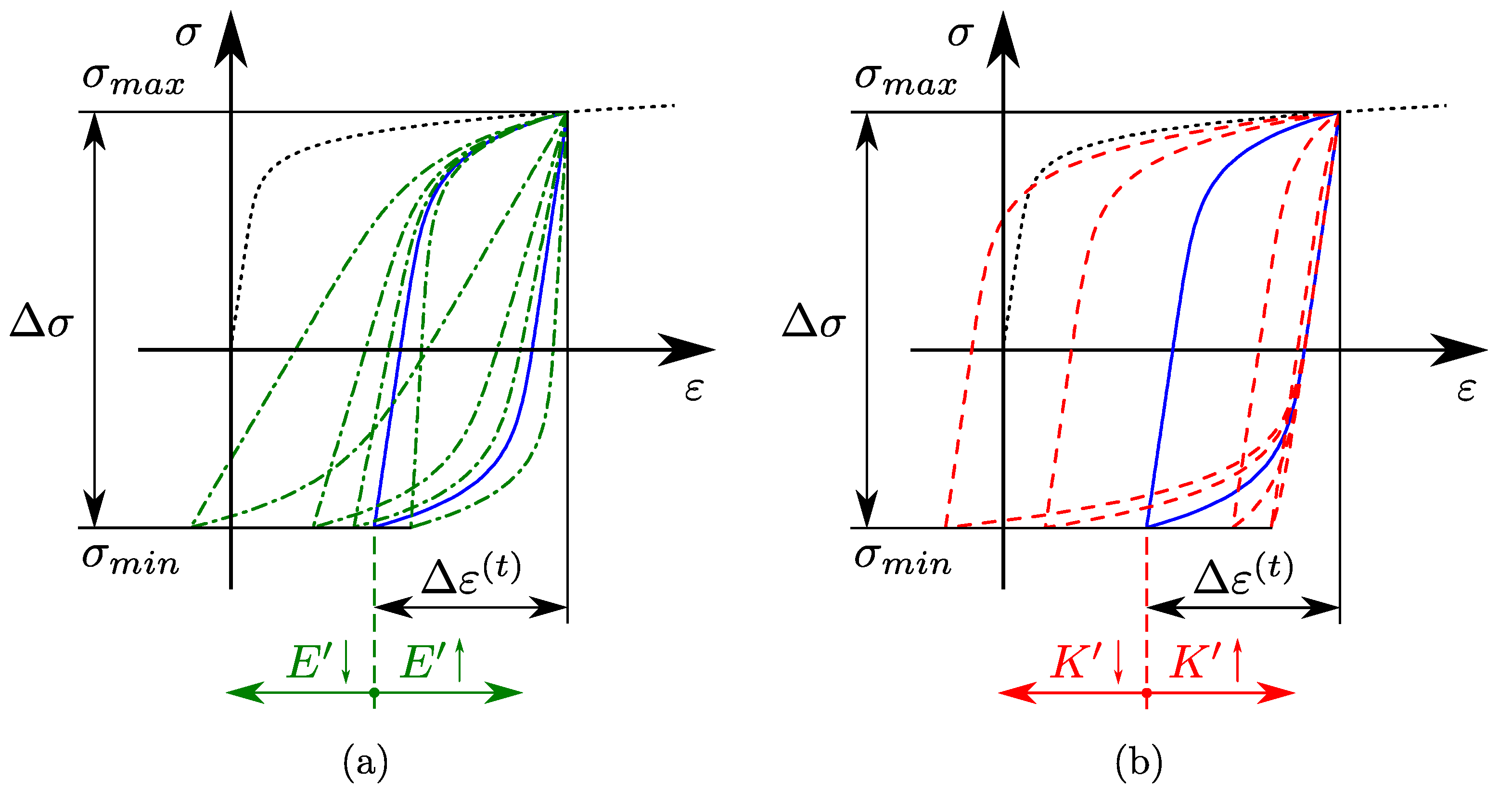The influence of the two parameters on the shape of the cyclic stabilized hysteresis loop is depicted in Figure 21.

Concerning Figure 21, the hysteresis loop depicted in blue constitutes the reference state. Varying $E^{\prime }$, as shown in Figure 21a, alters the elastic SED $\Delta W^{\left(e\right)}$, while the plastic SED $\Delta W^{\left(p\right)}$ is unaffected. Then again, modulating $K^{\prime }$ changes $\Delta W^{\left(p\right)}$, while $\Delta W^{\left(e\right)}$ remains virtually unchanged, as depicted in Figure 21b.

The difference in strain response between the uniaxial and multiaxial stress state can be interpreted as some kind of constraint, which can be considered by a local change of stiffness in the volume element. In order to quantitatively describe this variation of stiffness, the modulation factors ${\xi }_{ij,k}^{\left(e\right)}$ and ${\xi }_{ij,k}^{\left(p\right)}$ are defined according to Equations (24) and (25). Both parameters are based on the comparison between the respective strain component $\Delta {\tilde{\epsilon }}_{ij,k}^{\left(e\right)}$ or $\Delta {\tilde{\epsilon }}_{ij,k}^{\left(p\right)}$ in the present multiaxial stress state and the corresponding hypothetical uniaxial strain component.

$${\xi }_{ij,k}^{\left(e\right)}=\frac{\Delta {\tilde{\sigma }}_{ij,k}}{E^{\prime }·\Delta {\tilde{\epsilon }}_{ij,k}^{\left(e\right)}}$$

(24)

$${\xi }_{ij,k}^{\left(p\right)}=\frac{\Delta {\tilde{\sigma }}_{ij,k}}{2^{1-n^{\prime }}·K^{\prime }·{\left[\Delta {\tilde{\epsilon }}_{ij,k}^{\left(p\right)}\right]}^{n^{\prime }}}$$

(25)

Utilizing ${\xi }_{ij,k}^{\left(e\right)}$ and ${\xi }_{ij,k}^{\left(p\right)}$, the stress–strain relationship given in Equation (26) is defined, which yields the total strain $\Delta {\tilde{\epsilon }}_{ij,k}^{\left(t\right)}$ in the multiaxial stress state consistent with Equation (23).

$$\Delta {\tilde{\epsilon }}_{ij,k}^{\left(t\right)}=\Delta {\tilde{\epsilon }}_{ij,k}^{\left(e\right)}+\Delta {\tilde{\epsilon }}_{ij,k}^{\left(p\right)}=\frac{\Delta {\tilde{\sigma }}_{ij,k}}{{\xi }_{ij,k}^{\left(e\right)}·E^{\prime }}+2{\left(\frac{\Delta {\tilde{\sigma }}_{ij,k}}{2·{\xi }_{ij,k}^{\left(p\right)}·K^{\prime }}\right)}^{\frac{1}{n^{\prime }}}$$

(26)

As the stress–strain relation for the individual components of the multiaxial stress state is now defined according to Equation (26), the elastic and plastic SED contributions can be evaluated. At first, the calculation of the respective SED parts is carried out for a stress ratio of $R=0$, independent of the effective stress ratio $R_{eff,ij,k}$. Combining Equation (26) with trivial geometrical observations based on Figure 2, the total SED $\Delta W_{ij,k,R=0}^{\left(t\right)}$ is evaluated according to Equation (27).

$$\Delta W_{ij,k,R=0}^{\left(t\right)}=\Delta {\tilde{\sigma }}_{ij,k}·\Delta {\tilde{\epsilon }}_{ij,k}^{\left(t\right)}-{\int }_0^{\Delta {\tilde{\sigma }}_{ij,k}}\left[\frac{\widehat{\sigma }}{{\xi }_{ij,k}^{\left(e\right)}·E^{\prime }}+2{\left(\frac{\widehat{\sigma }}{2·{\xi }_{ij,k}^{\left(p\right)}·K^{\prime }}\right)}^{\frac{1}{n^{\prime }}}\right]d\widehat{\sigma }$$

(27)

Subsequently, the plastic SED $\Delta W_{ij,k,R=0}^{\left(p\right)}$ is calculated following Equation (28).

$$\Delta W_{ij,k,R=0}^{\left(p\right)}=\Delta {\tilde{\sigma }}_{ij,k}·\Delta {\tilde{\epsilon }}_{ij,k}^{\left(t\right)}-2{\int }_0^{\Delta {\tilde{\sigma }}_{ij,k}}\left[\frac{\widehat{\sigma }}{{\xi }_{ij,k}^{\left(e\right)}·E^{\prime }}+2{\left(\frac{\widehat{\sigma }}{2·{\xi }_{ij,k}^{\left(p\right)}·K^{\prime }}\right)}^{\frac{1}{n^{\prime }}}\right]d\widehat{\sigma }$$

(28)

The elastic SED $\Delta W_{ij,k,R=0}^{\left(e\right)}$ represents the difference between the total and the plastic SED, as given by Equation (29).

$$\Delta W_{ij,k,R=0}^{\left(e\right)}=\Delta W_{ij,k,R=0}^{\left(t\right)}-\Delta W_{ij,k,R=0}^{\left(p\right)}={\int }_0^{\Delta {\tilde{\sigma }}_{ij,k}}\left[\frac{\widehat{\sigma }}{{\xi }_{ij,k}^{\left(e\right)}·E^{\prime }}+2{\left(\frac{\widehat{\sigma }}{2·{\xi }_{ij,k}^{\left(p\right)}·K^{\prime }}\right)}^{\frac{1}{n^{\prime }}}\right]d\widehat{\sigma }$$

(29)

Finally, the SED components are calculated for the effective stress ratio $R_{eff,ij,k}$, which is induced by the mean stress relaxation during cyclic loading and is given by Equation (30).

$$R_{eff,ij,k}=\frac{{\tilde{\sigma }}_{ij,min,k}}{{\tilde{\sigma }}_{ij,max,k}}$$

(30)

As the plastic SED relies solely on the shape of the cyclic stabilized hysteresis loop, it follows that $\Delta W_{ij,k}^{\left(p\right)}$ at $R_{eff,ij,k}$ equals $\Delta W_{ij,k,R=0}^{\left(p\right)}$ given by Equation (28).

The elastic SED $\Delta W_{ij,k}^{\left(e\right)}$ depends on $R_{eff,ij,k}$ and is evaluated according to Equation (31).

$$\Delta W_{ij,k}^{\left(e\right)}=\left\{\begin{array}{cc}\Delta W_{ij,k,R=0}^{\left(e\right)}+{\tilde{\sigma }}_{ij,min,k}·\Delta {\tilde{\epsilon }}_{ij,k}^{\left(t\right)}\hfill & 0\le R_{eff,ij,k}\le 1\hfill \\ {\int }_0^{\left|{\tilde{\sigma }}_{ij,min,k}\right|}\left[\frac{\widehat{\sigma }}{{\xi }_{ij,k}^{\left(e\right)}·E^{\prime }}+2{\left(\frac{\widehat{\sigma }}{2·{\xi }_{ij,k}^{\left(p\right)}·K^{\prime }}\right)}^{\frac{1}{n^{\prime }}}\right]d\widehat{\sigma }+{\int }_0^{{\tilde{\sigma }}_{ij,max,k}}\left[\frac{\widehat{\sigma }}{{\xi }_{ij,k}^{\left(e\right)}·E^{\prime }}+2{\left(\frac{\widehat{\sigma }}{2·{\xi }_{ij,k}^{\left(p\right)}·K^{\prime }}\right)}^{\frac{1}{n^{\prime }}}\right]d\widehat{\sigma }\hfill & -\infty \le R_{eff,ij,k}<0\hfill \end{array}\right.$$

(31)

As the elastic and plastic contributions are evaluated, the total SED $\Delta W_{ij,k}^{\left(t\right)}$ is calculated as their superposition following Equation (32).

$$\Delta W_{ij,k}^{\left(t\right)}=\Delta W_{ij,k}^{\left(e\right)}+\Delta W_{ij,k}^{\left(p\right)}$$

(32)

Figure 22 summarizes the individual steps of the approximation methodology in a graphical way.

The last step in the calculation procedure for the element $C_k$ constitutes the evaluation of the strain energy. Utilizing the element volume $V_{Element,k}$ derived from the finite element model, the elastic, plastic and total strain energy contributions are evaluated following Equations (33)–(35).

$$\Delta E_{ij,k}^{\left(e\right)}=\Delta W_{ij,k}^{\left(e\right)}·V_{Element,k}$$

(33)

$$\Delta E_{ij,k}^{\left(p\right)}=\Delta W_{ij,k}^{\left(p\right)}·V_{Element,k}$$

(34)

$$\Delta E_{ij,k}^{\left(t\right)}=\Delta W_{ij,k}^{\left(t\right)}·V_{Element,k}$$

(35)

The approximation framework according to Equations (14)–(16) and (18)–(35) is utilised to calculate the strain energy terms for each of the n finite elements within $\mathsf{\Omega }$. In order to calculate the SED terms averaged over the whole control volume, the individual strain energy contributions of each element are summed and finally divided by the sum of the element volumes within $\mathsf{\Omega }$. To preserve consistency with the finite element simulations utilised to validate the approximation framework, it should be noted that each strain energy term $\Delta E_{ij,k}^{\left(e\right)}$ or $\Delta E_{ij,k}^{\left(p\right)}$ contributes either positively or negatively to the total sum. The respective sign depends on the ones of the stress and strain components and is implemented based on their product. As the resulting plastic strain energy is dissipated, the resulting sum of the individual contributions is defined as positive by convention. Finally, Equations (36)–(38) yield the averaged SED terms considering all n elements within $\mathsf{\Omega }$, where $sgn$ represents the signum function.

$$\Delta {\overline{W}}^{\left(e\right)}=\frac{{\sum }_{k=1}^n{\sum }_{i=1}^3{\sum }_{j=1}^{3}sgn\left[\Delta {\tilde{\sigma }}_{ij,k}·\Delta {\tilde{\epsilon }}_{ij,k}^{\left(e\right)}\right]·\Delta E_{ij,k}^{\left(e\right)}}{{\sum }_{k=1}^n{V}_{Element,k}}$$

(36)

$$\Delta {\overline{W}}^{\left(p\right)}=\frac{\left|{\sum }_{k=1}^n{\sum }_{i=1}^3{\sum }_{j=1}^{3}sgn\left[\Delta {\tilde{\sigma }}_{ij,k}·\Delta {\tilde{\epsilon }}_{ij,k}^{\left(p\right)}\right]·\Delta E_{ij,k}^{\left(p\right)}\right|}{{\sum }_{k=1}^n{V}_{Element,k}}$$

(37)

$$\Delta {\overline{W}}^{\left(t\right)}=\Delta {\overline{W}}^{\left(e\right)}+\Delta {\overline{W}}^{\left(p\right)}$$

(38)

Equation (38) concludes the definition of the introduced elastic–plastic approximation framework. In order to prove its capabilities for the elastic–plastic fatigue assessment of notched and defect-afflicted cast steel components, the following section validates the methodology.

3.5. Validation of the Elastic–Plastic Approximation Framework

The obtained results of the approximation framework defined in Section 3.4 are validated utilizing non-linear finite element analyses. The validation procedure covers the non-linear simulations of the V-notched fatigue samples, which served as an experimental basis for the evaluation of the elastic–plastic design limit curve presented in Section 3.3. Both specimen geometries possessing notch opening angles of $2\alpha ={45}^{\circ }$ and $2\alpha ={135}^{\circ }$ are assessed by the presented elastic–plastic approximation framework, covering all experimentally tested stress ranges $\Delta \sigma$ and stress ratios R. The elastic and plastic SED terms $\Delta {\overline{W}}^{\left(e\right)}$ and $\Delta {\overline{W}}^{\left(p\right)}$, as well as the total SED $\Delta {\overline{W}}^{\left(t\right)}$, are evaluated and compared to the ones obtained by the finite element analyses. 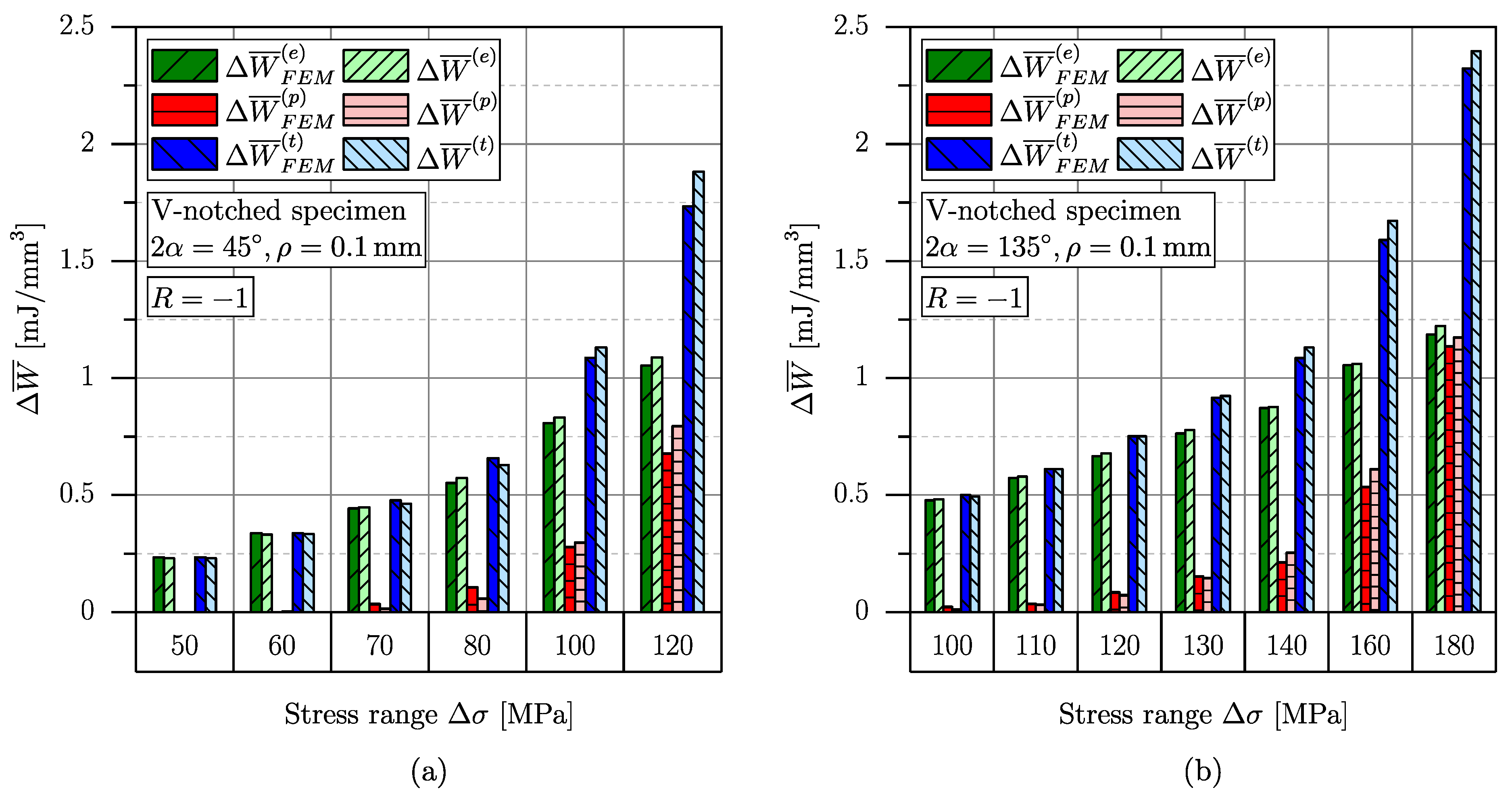Figure 23 depicts a comparison of the non-linear simulation results and those obtained by the elastic–plastic approximation framework for both specimen geometries and a stress ratio of $R=-1$.

Reflecting the results depicted in Figure 23, a sound accordance of the results obtained by elastic–plastic finite element analyses $\Delta {\overline{W}}_{FEM}$ and the ones derived by the presented approximation framework $\Delta \overline{W}$ can be perceived. Both the elastic and plastic SED components show only a small deviation from the simulation results, therefore leading to a quite satisfying approximation of the total SED. Comparing (a) and (b) in Figure 23, the effect of the notch geometry can be perceived clearly. Considering loading of both notch geometries under an identical stress range $\Delta \sigma$, the elastic and plastic SED contributions possess higher values at a notch opening angle of $2\alpha ={45}^{\circ }$ than at $2\alpha ={135}^{\circ }$. To further investigate the capabilities of the introduced assessment method, the stabilized hysteresis loops evaluated by non-linear simulation and the presented approximation procedure are compared to each other. 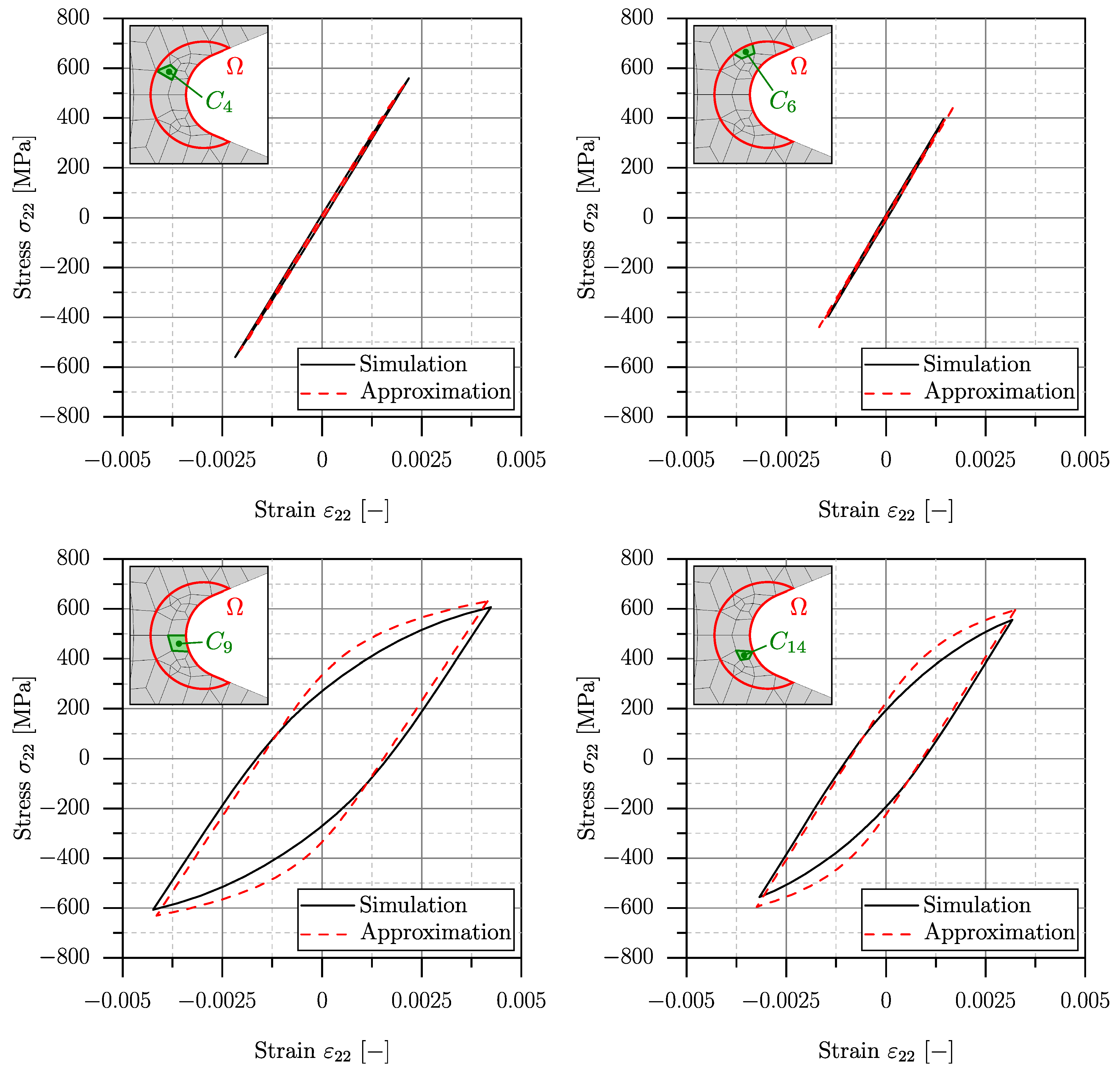Figure 24 depicts respective hysteresis loops for the stress component ${\sigma }_{22}$ parallel to the specimen axis which yields the main contribution to $\Delta {\overline{W}}^{\left(t\right)}$.

Table 7. Average deviations obtained by the applied assessment methodologies.

$2\mathit{\alpha }{[}^{\circ }]$	$\mathit{R}[-]$	${\mathbf{\Delta }}_{\mathit{unsigned}}[\%]$	${\mathbf{\Delta }}_{\mathit{signed}}[\%]$	${\mathbf{\Delta }}_{\mathit{RMS}}[\%]$
	$-1$	3.9	+0.3	4.5
45	0	6.4	$-5.3$	6.9
	0.5	10.7	$-5.0$	11.7
	$-1$	2.1	+1.7	2.9
135	0	10.9	$-10.6$	12.0
	0.5	6.9	+5.9	10.7

summarizes the comparison between elastic–plastic simulations and the approximation framework for the investigated notch geometries and stress ratios in terms of the unsigned and signed deviations ${\Delta }_{unsigned}$ and ${\Delta }_{signed}$, as well as the root mean square error ${\Delta }_{RMS}$; see Equations (39)–(41).

$${\Delta }_{unsigned}=\frac{1}{n}·\sum _{i=1}^n\frac{\left|\Delta {\overline{W}}_i^{\left(t\right)}-\Delta {\overline{W}}_{FEM,i}^{\left(t\right)}\right|}{\Delta {\overline{W}}_{FEM,i}^{\left(t\right)}}·100\%$$

(39)

$${\Delta }_{signed}=\frac{1}{n}·\sum _{i=1}^n\frac{\Delta {\overline{W}}_i^{\left(t\right)}-\Delta {\overline{W}}_{FEM,i}^{\left(t\right)}}{\Delta {\overline{W}}_{FEM,i}^{\left(t\right)}}·100\%$$

(40)

$${\Delta }_{RMS}=\sqrt{\frac{1}{n}·\sum _{i=1}^n{\left[\frac{\Delta {\overline{W}}_i^{\left(t\right)}-\Delta {\overline{W}}_{FEM,i}^{\left(t\right)}}{\Delta {\overline{W}}_{FEM,i}^{\left(t\right)}}·100\%\right]}^2}$$

(41)

The depicted values in Table 7 confirm the sound applicability of the presented approximation methodology as a maximum root mean square deviation of only $12.0\%$ is achieved. To put this value into perspective, it should be noted that this energy-based deviation translates to $5.8\%$ in terms of stress when considering a hypothetical linear–elastic material behaviour. In order to demonstrate the difference in numerical efficiency, Figure 25 depicts a comparison of the computation time needed for total strain energy density calculation using non-linear finite element analyses and the elastic–plastic approximation framework. The depicted values summarize the evaluation effort of all experimentally tested stress ranges $\Delta \sigma$.

Considering Figure 25, the enhanced numerical efficiency obtained by the presented elastic–plastic approximation framework can be perceived clearly. Regarding the non-linear finite element analyses, the evaluation of the cyclic stabilized material behaviour constitutes the main contribution to the observed computation times. Due to the occurring elastic–plastic deformations, the investigated loads have to be applied in small increments in order to achieve an equilibrium condition in the implicit simulations. As the presented approximation procedure is solely based upon a quasi-static linear–elastic finite element analysis, no incremental load stepping has to be applied, which significantly reduces numerical efforts and therefore computation time. Hence, the application of the established approximation method enables a calculation of the total strain energy density which is on average approximately 400 times faster compared to non-linear finite element analyses.

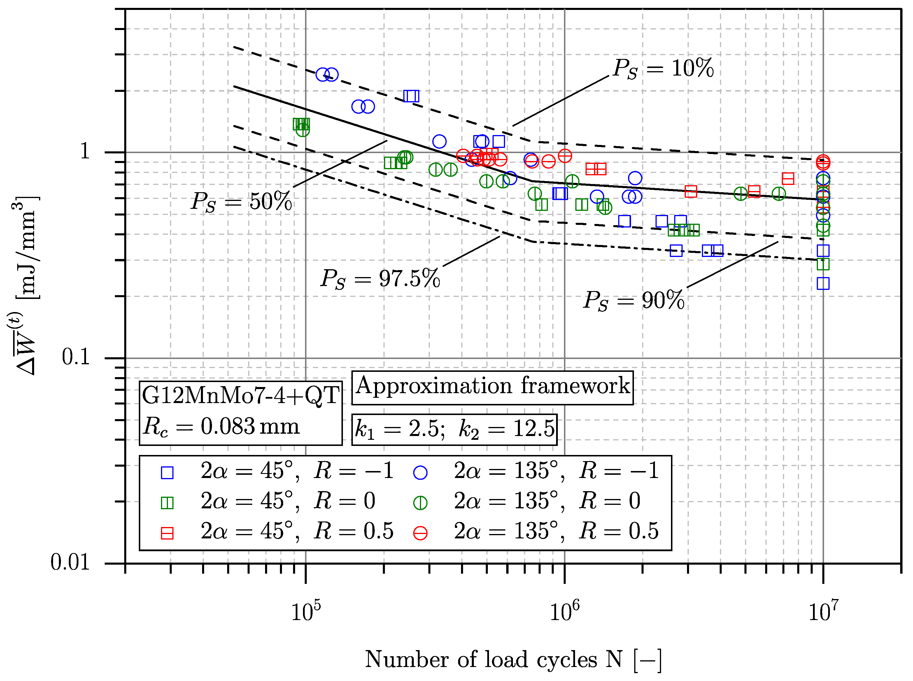
Finally, Figure 26 depicts the approximation results for the notched specimens with $2\alpha ={45}^{\circ }$ and $2\alpha ={135}^{\circ }$ tested at $R=-1$, $R=0$ and $R=0.5$, which merge well into the previously evaluated scatter band; compare Figure 18 as a reference.

3.6. Calculation of the Elastic–Plastic Strain Energy Density of Bulk and Surface Defects

As the established approximation framework is validated, the methodology is applied to assess the fatigue strength of large-scale specimens affected by bulk and surface imperfections.

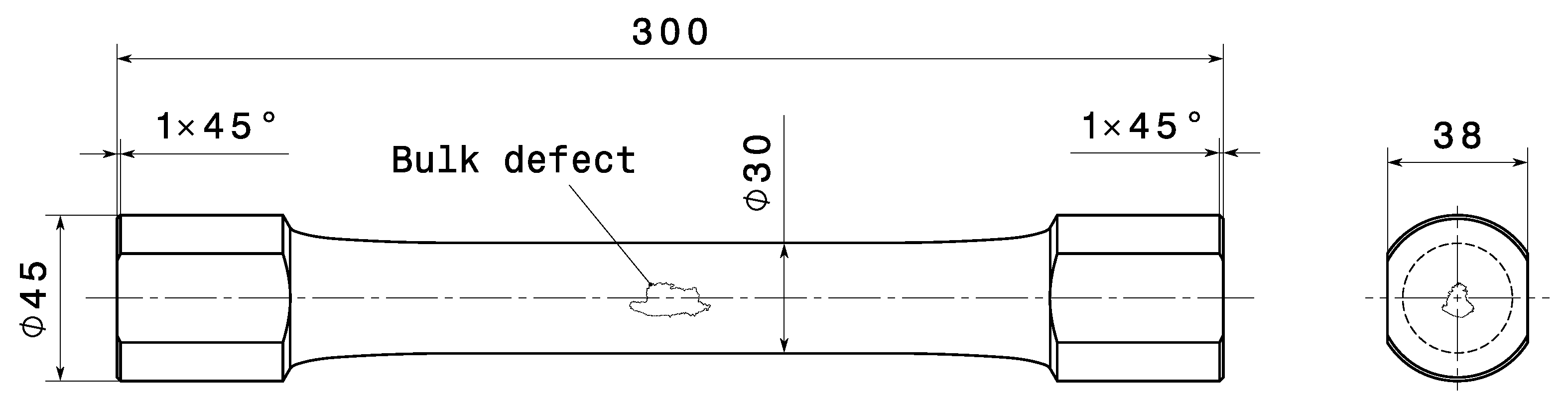
Starting with bulk defect-afflicted cast steel specimens, the consistency of the presented elastic–plastic approximation method in the linear–elastic fatigue regime is investigated at first. Therefore, the numerical results of the large-scale specimens given in [10] are reassessed utilizing Abaqus^® 2021 and plane strain elements of the type CPE6/CPE8. Twenty defect contours are considered, including ten specimens tested at $R=-1$ and $R=0$, respectively. Furthermore, the selected specimens tested at $R=0.5$ which are reported in Section 2.2 are also included. A stress range of $\Delta \sigma =1$ MPa acting in the cross-section with a diameter of 30 mm is utilised in order to evaluate the elastic SED $\Delta {\overline{W}}_{DEF,97.5\%}^{\left(e\right)}$ according to [10]. The evaluation of $\Delta {\overline{W}}_{DEF,97.5\%}^{\left(e\right)}$ includes the partitioning of individual control volumes along the respective defect contour which corresponds to Method 1 reported in a preceding study [104]. Based on the investigated control volumes, the fatigue parameter $\Delta {\overline{W}}_{DEF,97.5\%}^{\left(e\right)}$ is evaluated, which is defined as the averaged SED value that exceeds $97.5\%$ of all derived values along the defect perimeter [10]. Subsequent to the evaluation of $\Delta {\overline{W}}_{DEF,97.5\%}^{\left(e\right)}$, the derived linear–elastic stress fields in the investigated control volumes along the defect perimeter are assessed by the methodology introduced in Section 3.4 and evaluated as a $97.5\%$ elastic–plastic SED exceedance limit $\Delta {\overline{W}}_{DEF,97.5\%}^{\left(t\right)}$. 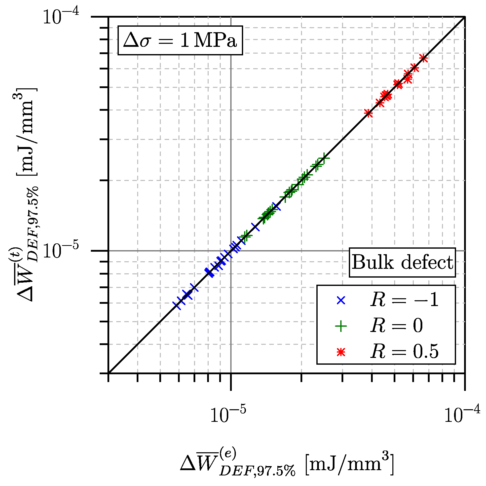Figure 27 depicts a comparison of $\Delta {\overline{W}}_{DEF,97.5\%}^{\left(e\right)}$ and $\Delta {\overline{W}}_{DEF,97.5\%}^{\left(t\right)}$ for a gross stress of $\Delta \sigma =1$ MPa.

The consistency between the approximation framework and the fatigue assessment method introduced in [10] in the linear–elastic fatigue regime can be perceived clearly. Nearly all evaluated data points are on the diagonal line, indicating a match of the calculated SED values. The derived statistical deviations possess values of ${\Delta }_{unsigned}=0.56\%$, ${\Delta }_{signed}=-0.19\%$ and ${\Delta }_{RMS}=1.24\%$, confirming the sound applicability of the elastic–plastic approximation framework in the linear–elastic fatigue regime.

Subsequent to the consistency check, the elastic–plastic approximation framework is utilised for the elastic–plastic fatigue assessment of the bulk defect-afflicted large-scale specimens as reported in Section 2.2 and [10]. This includes the evaluation of the linear–elastic stress fields in the control volumes along the defect contour. Two-dimensional finite element models subjected to a gross stress of $\Delta \sigma =1$ MPa are used, featuring plane strain elements of type CPE6/CPE8. Considering the stress ranges investigated in the respective experiments, the total SED $\Delta {\overline{W}}_{DEF,97.5\%}^{\left(t\right)}$ is evaluated at increased stress levels of hundreds of Megapascals of gross stress under uniaxial tension, utilizing an exceedance limit of $97.5\%$ along the defect contour in accordance with [10]. It should be noted that each defect is assessed in terms of the two radiographs captured prior to testing. Hence, the energy-based fatigue assessment method yields two values of $\Delta {\overline{W}}_{DEF,97.5\%}^{\left(t\right)}$ for each individual defect.

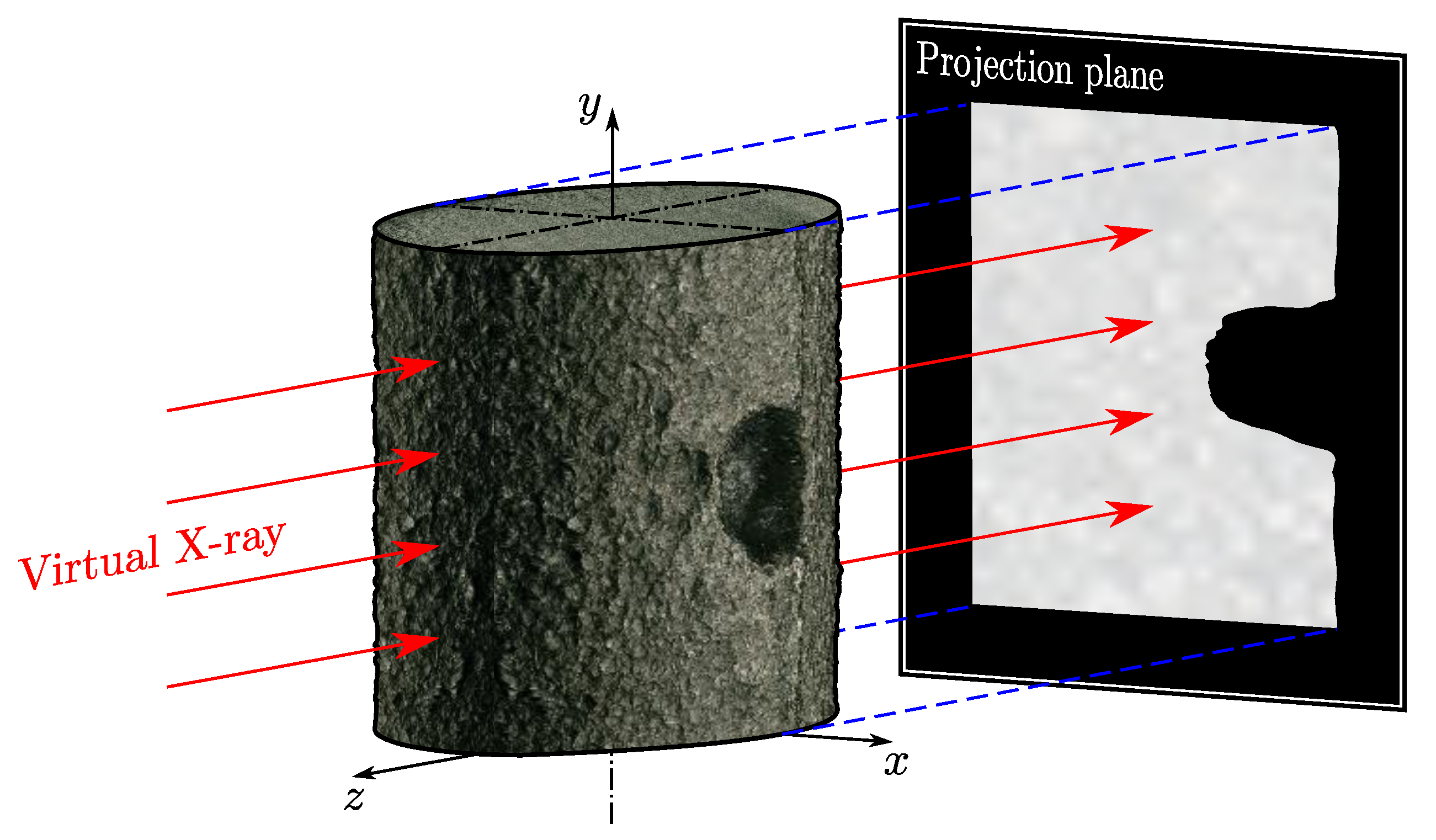
Concerning the surface defect-afflicted specimens presented in Section 2.3, the energy-based fatigue assessment considers the three-dimensional image stacks of the individual defect structures, which were captured prior to testing. The image stack contains the spatial coordinates of the defect contour which are processed for projected edge detection. The scripted procedure includes the alignment of the defect structure on the specimen. The three-dimensional point cloud is utilised to derive a virtual radiograph by projecting the volumetric surface defect onto a plane which is parallel to the specimen axis, as shown in Figure 28.

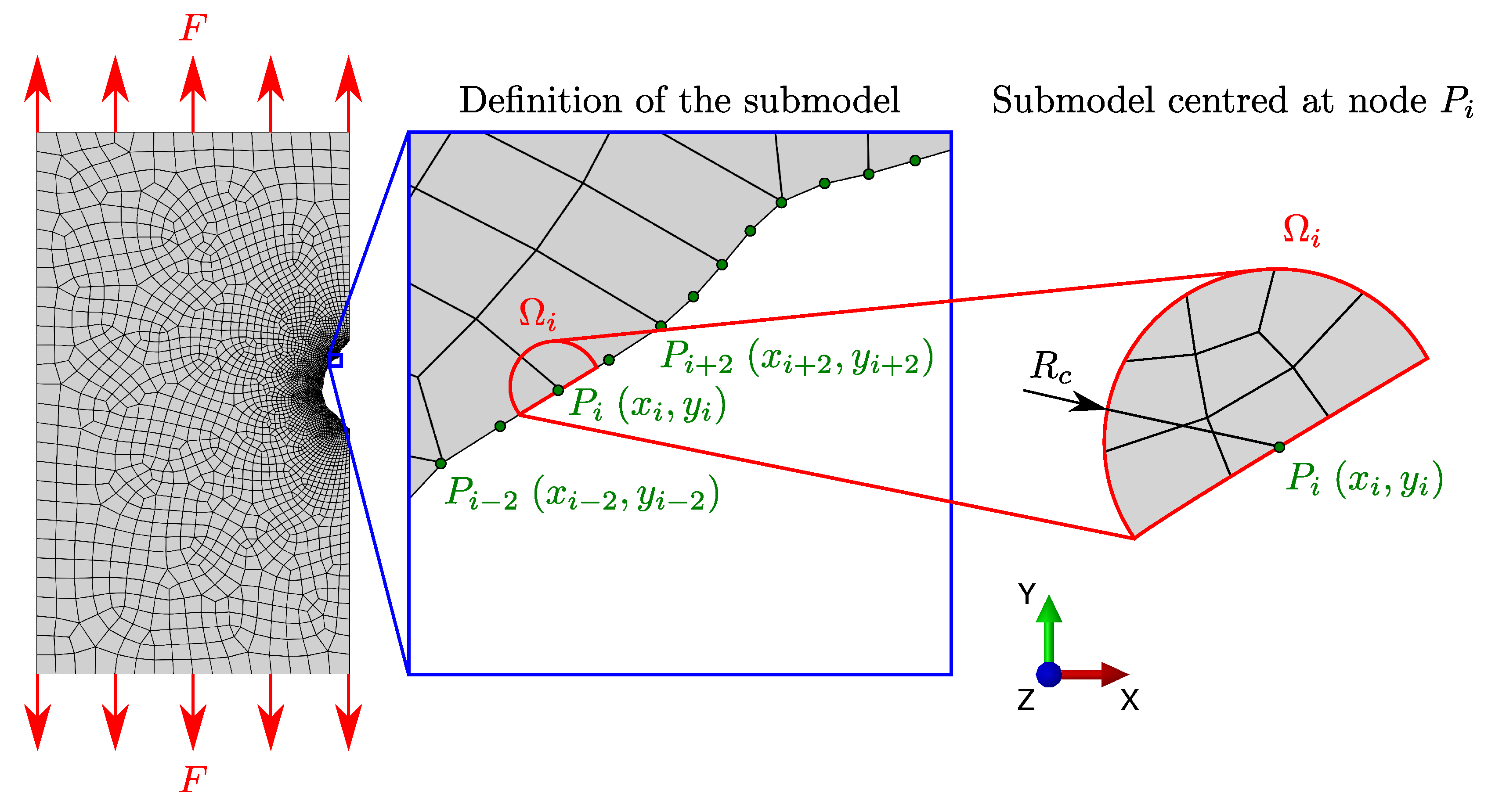
Based on this planar edge projection, a linear–elastic plane strain finite element model is set up. Analogous to the assessment of the bulk defect-afflicted specimens, the finite element submodeling technique is utilised to derive the linear–elastic stress tensors of each element within the control volume ${\mathsf{\Omega }}_i$. Subsequently, ${\mathsf{\Omega }}_i$ is assessed following the elastic–plastic approximation framework presented in Section 3.4. As the total SED is evaluated for ${\mathsf{\Omega }}_i$, the numerical procedure is repeated until the whole defect contour has been assessed. As in the case of the bulk defect-afflicted specimens, the fatigue effective total SED $\Delta {\overline{W}}_{DEF,97.5\%}^{\left(t\right)}$ is derived by considering an exceedance limit of $97.5\%$. Figure 29 exemplarily depicts the implemented finite element submodeling technique.

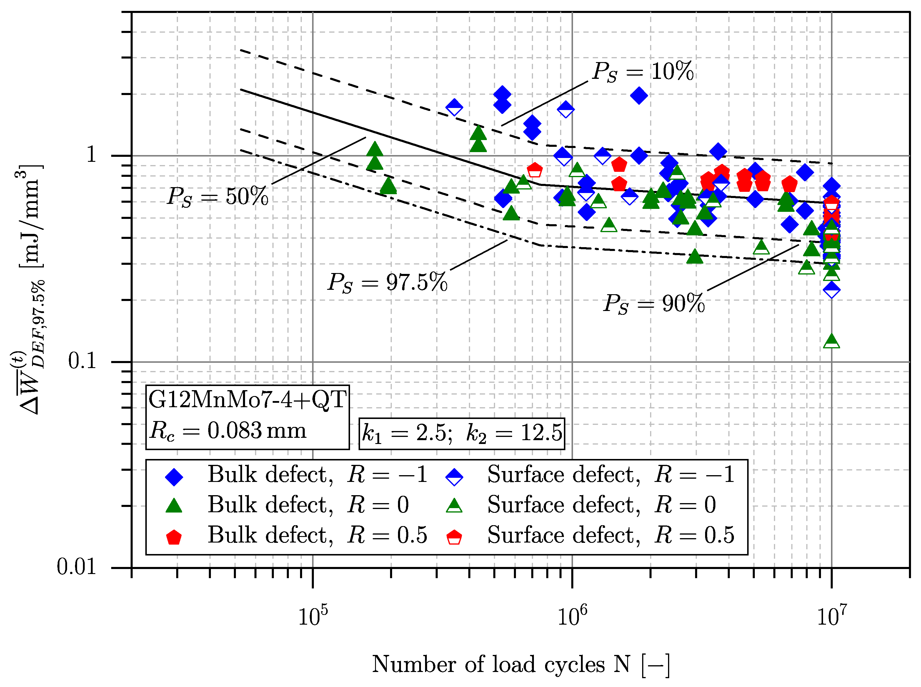
As the investigated bulk and surface defects are assessed by the elastic–plastic approximation framework, the evaluated data points $\Delta {\overline{W}}_{DEF,97.5\%}^{\left(t\right)}$ are plotted as a function of the experimentally derived numbers of load cycles. Figure 30 depicts the original scatter band, as evaluated in Section 3.3, as well as the fatigue assessment results of the defect-afflicted large-scale specimens.

Concerning Figure 30, the elastic–plastic fatigue assessment of bulk and surface defect-afflicted cast steel specimens yields satisfying results, as nearly all data points fall within the scatter band derived by small-scale specimen experiments. This highlights the ability of the total strain energy density concept to assess arbitrarily notched geometrical features. Bearing in mind that each data point in Figure 30 represents only a planar projection of a complexly shaped spatial imperfection, the depicted results also prove the presented approximation framework as an engineering-feasible fatigue assessment methodology. Focusing on the data points at a stress ratio of $R=0.5$, the implementation of the mean stress relaxation and the resulting effective stress ratio is emphasized, which constitutes a significant improvement in prediction accuracy compared to the linear–elastic SED concept. As associated numerical efforts are substantially reduced compared to non-linear finite element analyses, the elastic–plastic approximation method represents a promising tool to assess arbitrarily shaped defect geometries. In order to minimize computational efforts for complex defect geometries or imperfection networks even further, the implementation of a free-mesh approach as reported in [104] is encouraged for future work. Moreover, the presented elastic–plastic approximation framework can be expanded from planar case studies towards spatial fatigue assessment as well.

4. Conclusions

The present paper focuses on the elastic–plastic energy-based fatigue assessment of notched and imperfective cast steel components. Based on the conducted experimental and numerical investigations, the following scientific conclusions are drawn:

• A design limit curve for the high-strength cast steel alloy G12MnMo7-4+QT was evaluated based on the elastic–plastic strain energy density concept and non-linear finite element analyses. The evaluated design limit curve considers the results of high-cycle fatigue experiments of three different specimen geometries tested at stress ratios of $R=-1$, $R=0$ and $R=0.5$. Implementation of the elastic–plastic material behaviour results in a significant improvement of prediction accuracy compared to the linear–elastic assessment conducted in a previous study, as the considered experimental results merge into a unique narrow scatter band which is characterized by a scatter index of $1:T_{\Delta {\overline{W}}^{\left(t\right)}}=2.43$.
• The effect of mean stress relaxation results in the formation of an effective stress ratio that is smaller than the stress ratio of the applied load and generally tends towards $R=-1$. For cyclic loading at stress ratios of $R\ge 0$, this leads to a decrease of the total SED compared to the results of the linear–elastic SED concept.
• A novel elastic–plastic approximation approach to evaluate the total strain energy density was presented. The framework facilitates the rapid assessment of the elastic–plastic stress and strain tensors in the cyclic stabilized material state, invoking only linear–elastic finite element analysis and low-cycle fatigue properties. Hence, numerical efficiency is significantly increased compared to time-consuming non-linear finite element analyses.
• Validation of the elastic–plastic approximation framework utilizing comprehensive elastic–plastic finite element analyses of two V-notched small-scale specimen geometries proved a sound agreement of obtained approximation and non-linear simulation results, showing an average root mean square deviation of only approximately eight percent.
• The fatigue assessment of bulk and surface defect-afflicted large-scale specimens utilizing the introduced elastic–plastic approximation method results in quite satisfying fatigue life calculations. A total of 56 defect-afflicted large-scale specimens tested at stress ratios of $R=-1$, $R=0$ and $R=0.5$ were investigated by the presented framework, yielding calculated fatigue life results which merge into the scatter band of the derived high-strength cast steel design fatigue curve.
• As the elastic–plastic approximation framework is solely based on linear–elastic simulations currently utilizing planar projections of complexly shaped spatial imperfections, cost and time expenses are significantly decreased compared to three-dimensional non-linear finite element simulations. Hence, the presented approximation methodology presents an engineering-feasible design tool to assess the fatigue strength of bulk and surface defect-afflicted cast steel components.