Stability of Heterogeneous Beams with Three Supports—Solutions Using Integral Equations


Abstract
:1. Introduction
2. Differential Equations
Governing Equations
3. Green Function for Three-Point BVPs
3.1. Green Function for FssF Beams
3.1.1. Calculation of the Green Function if
3.1.2. Calculation of the Green Function if
3.2. Green Function for FssP Beams
3.3. Green Function for PssP Beams
4. The Stability Problem of FssF, SssP and PssP Beams with Three Supports
4.1. Solution Procedures
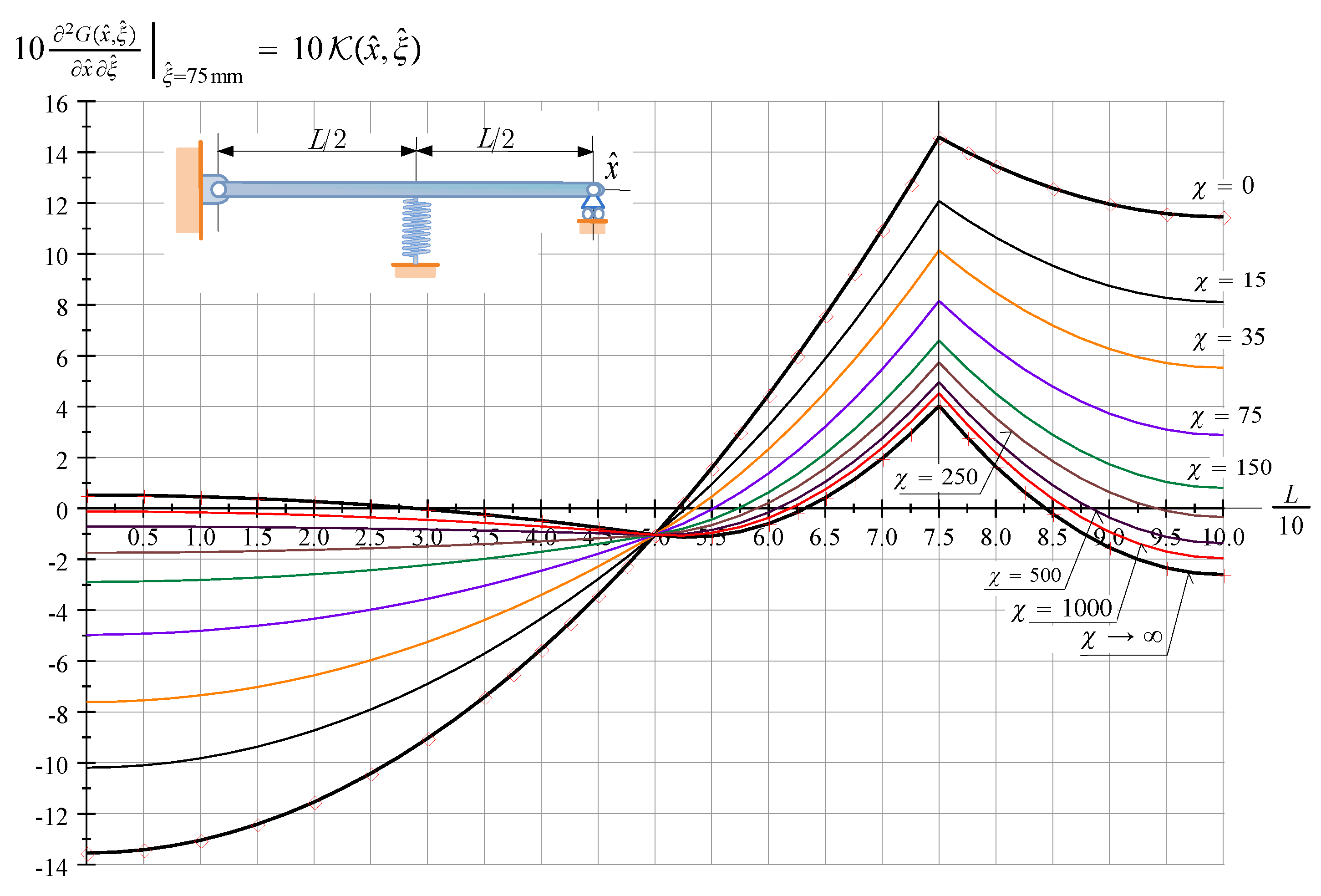
4.2. The Kernel for FssF Beams
4.3. The Kernel for FssP Beams
4.4. The Kernel for PssP Beams
5. Computational Results
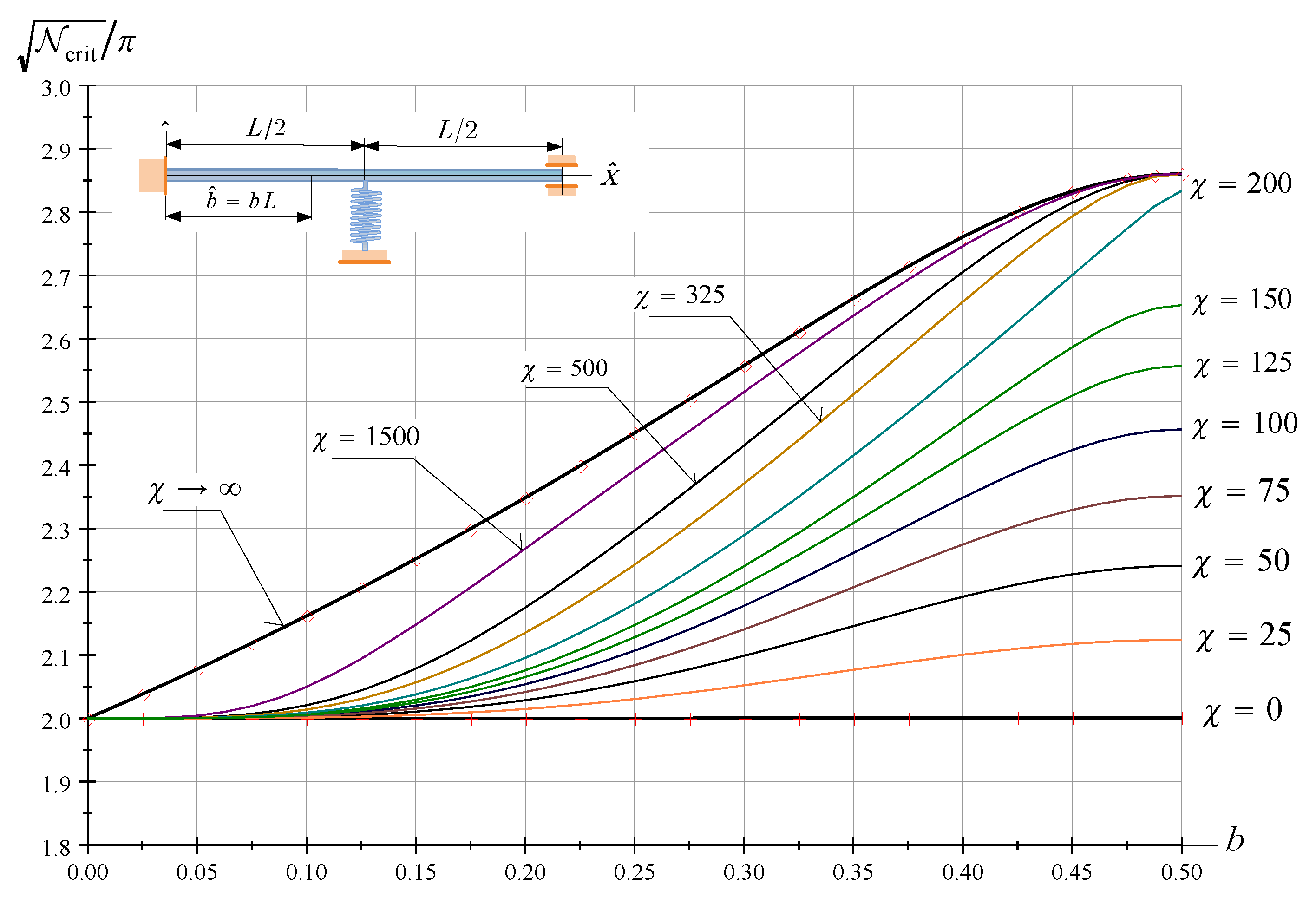
5.1. FssF Beams
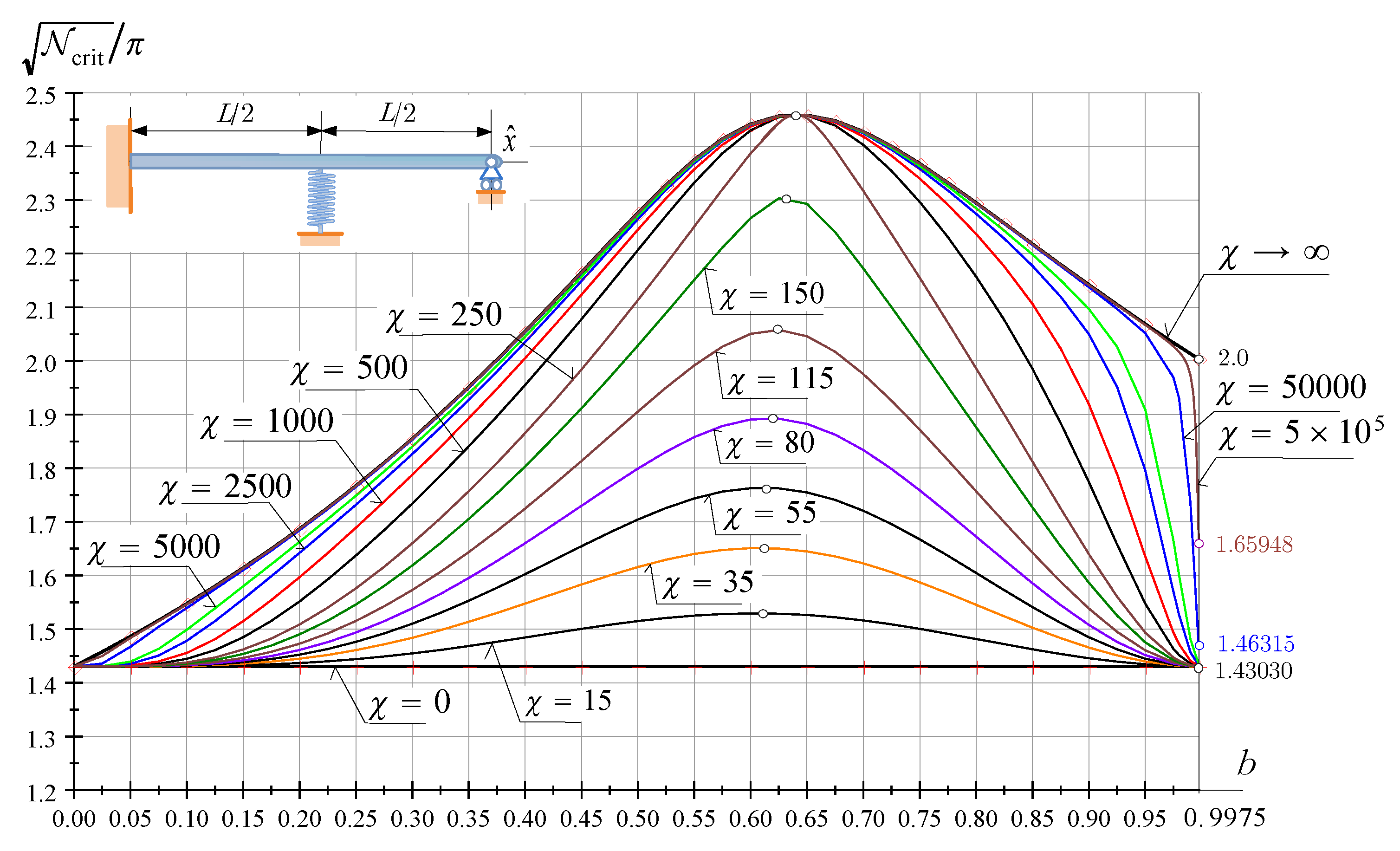
5.2. FssP Beams
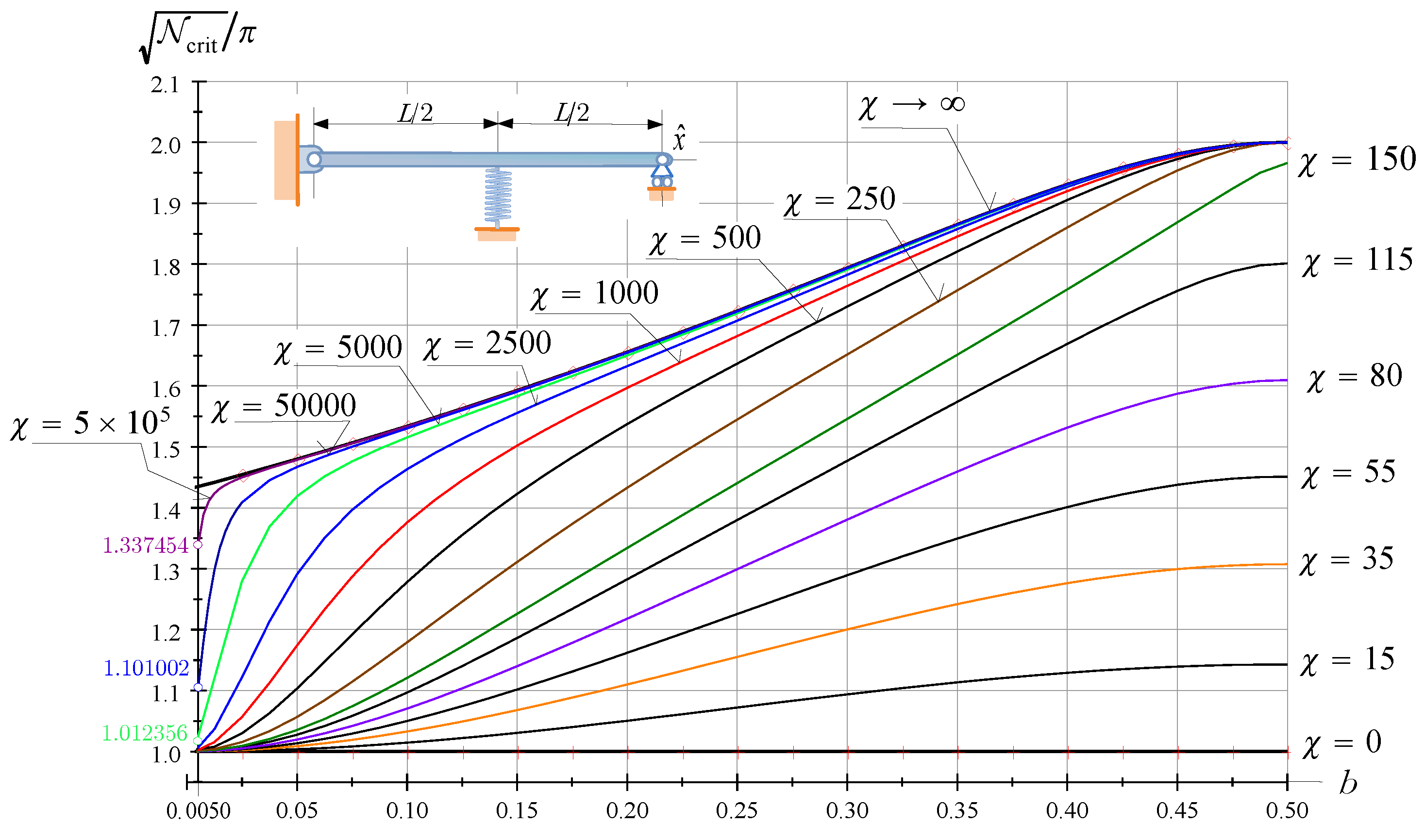
5.3. PssP Beams
6. Conclusions
Author Contributions
Funding
Data Availability Statement
Conflicts of Interest
Appendix A. Limit Cases
Appendix A.1. The Green Function for FrF Beams
Appendix A.2. The Green Function for FrP Beams
Appendix A.3. The Green Function for PrP Beams
Appendix A.4. The Kernel Function for FrF Beams
Appendix A.5. The Kernel Function for FrP Beams
Appendix A.6. The Kernel Function for PrP Beams
Appendix A.7. Characteristic Equations
References
- Jerath, S. Structural Stability Theory and Ppractice: Buckling of Columns, Beams, Plates and Shells; Wiley: Hoboken, NJ, USA, 2020. [Google Scholar]
- Wang, C.M.; Wang, C.Y.; Reddy, J.N. Exact Solutions for Buckling of Structural Members; CRC Press: Boca Raton, FL, USA, 2004. [Google Scholar]
- Lanzoni, L.; Tarantino, A.M. The bending of beams in finite elasticity. J. Elast. 2020, 139, 91–121. [Google Scholar] [CrossRef]
- O’Reilly, O.M.; Peters, D.M. On stability analyses of three classical buckling problems for the elastic strut. J. Elast. 2011, 105, 117–136. [Google Scholar] [CrossRef] [Green Version]
- Murawski, K. Technical Stability of Continuously Loaded Thin-Walled Slender Columns; Lulu Press: Morrisville, NC, USA, 2017. [Google Scholar]
- Murawski, K. Comparison of the known hypotheses of lateral buckling in the elastic-plastic states of thin-walled semi-slender columns. Int. J. Struct. Glass Adv. Mater. Res. 2020, 4, 233–253. [Google Scholar] [CrossRef]
- Murawski, K. Technical stability of very slender rectangular columns compressed by ball-and-socket joints without friction. Int. J. Struct. Glass Adv. Mater. Res. 2020, 4, 186–208. [Google Scholar] [CrossRef]
- Wahrhaftig, A.M.; Magalhães, K.M.M.; Brasil, R.M.L.R.F.; Murawski, K. Evaluation of mathematical solutions for the determination of buckling of columns under self-weight. J. Vib. Eng. Technol. 2020, 4, 233–253. [Google Scholar] [CrossRef]
- Adman, R.; Saidani, M. Elastic buckling of columns with end restraint effects. J. Constr. Steel Res. 2013, 87, 1–5. [Google Scholar] [CrossRef]
- Coşkun, S.B.; Atay, M.T. Determination of critical buckling load for elastic columns of constant and variable cross-sections using variational iteration method. Comput. Math. Appl. 2009, 58, 2260–2266. [Google Scholar] [CrossRef] [Green Version]
- Singh, K.V.; Li, G. Buckling of functionally graded and elastically restrained non-uniform columns. Compos. Part B Eng. 2009, 40, 393–403. [Google Scholar] [CrossRef]
- Khan, Y.; Al-Hayani, W. A nonlinear model arising in the buckling analysis and its new analytic approximate solution. Z. Naturforsch 2013, 68, 355–361. [Google Scholar] [CrossRef]
- Gupta, P.; Kumar, A. Effect of material nonlinearity on spatial buckling of nanorods and nanotubes. J. Elast. 2017, 126, 155–171. [Google Scholar] [CrossRef]
- Pelliciari, M.; Falope, F.O.; Lanzoni, L.; Tarantino, A.M. Theoretical and experimental analysis of the von Mises truss subjected to a horizontal load using a new hyperelastic model with hardening. Eur. J. Mech. A/Solids 2023, 97, 104825. [Google Scholar] [CrossRef]
- Anghel, V.; Mares, C. Numerical integral approaches for buckling analysis of straight beams. UPB Sci. Bull. Ser. D 2020, 82, 227–238. [Google Scholar]
- Virgin, L. Tailored buckling constrained by adjacent members. Structures 2018, 16, 20–26. [Google Scholar] [CrossRef]
- Harvey, P.S.; Virgin, L.N.; Tehrani, M.H. Buckling of elastic columns with second-mode imperfections. Meccanica 2019, 54, 1245–1255. [Google Scholar] [CrossRef]
- Green, G. An Essay on the Application of Mathematical Analysis to the Theories of Electricity and Magnetism; T. Wheelhouse: Notthingam, UK, 1828. [Google Scholar]
- Stakgold, I.; Holst, M. Green’s Functions and Boundary Value Problems; John Wiley & Sons: Hoboken, NJ, USA, 2011. [Google Scholar] [CrossRef]
- Li, X.; Zhao, X.; Li, Y. Green’s functions of the forced vibration of Timoshenko beams with damping effect. J. Sound Vib. 2014, 333, 1781–1795. [Google Scholar] [CrossRef]
- Bocher, M. Boundary problems and Green’s functions for linear differential and difference equations. Ann. Math. 1911–1912, 13, 71–88. [Google Scholar] [CrossRef]
- Collatz, L. Eigenwertaufgaben mit Technischen Anwendungen; Russian Edition in 1968; Akademische Verlagsgesellschaft Geest & Portig K.G.: Leipzig, Germany, 1963. [Google Scholar]
- Collatz, L. The Numerical Treatment of Differential Equations, 3rd ed.; Springer: Berlin/Heidelberg, Germany, 1966. [Google Scholar]
- Obádovics, J.G. On the Boundary and Initial Value Problems of Differental Equation Systems. Ph.D. Thesis, Hungarian Academy of Sciences, Budapest, Hungary, 1967. (In Hungarian). [Google Scholar]
- Szeidl, G. Effect of the Change in Length on the Natural Frequencies and Stability of Circular Beams. Ph.D. Thesis, Department of Mechanics, University of Miskolc, Miskolc, Hungary, 1975. (In Hungarian). [Google Scholar]
- Murty, S.N.; Kumar, G.S. Three point boundary value problems for third order fuzzy differential equations. J. Chungcheong Math. Soc. 2006, 19, 101–110. [Google Scholar]
- Zhao, Z. Solutions and Green’s functions for some linear second-order three-point boundary value problems. Comput. Math. 2008, 56, 104–113. [Google Scholar] [CrossRef] [Green Version]
- Smirnov, S. Green’s function and existence of a unique solution for a third-order three-point boundary value problem. Math. Model. Anal. 2019, 24, 171–178. [Google Scholar] [CrossRef] [Green Version]
- Bouteraa, N.; Benaicha, S. Existence of solution for third-order three-point boundary value problem. Mathematica 2018, 60, 21–31. [Google Scholar] [CrossRef]
- Ertürk, V.S. A unique solution to a fourth-order three-point boundary value problem. Turk. J. Math. 2020, 44, 1941–1949. [Google Scholar] [CrossRef]
- Roman, S.; Stikonas, A. Third-order linear differential equation with three additional conditions and formula for Green’s function. Lith. Math. J. 2010, 50, 426–446. [Google Scholar] [CrossRef]
- Kiss, L.P.; Szeidl, G.; Messaoudi, A. Stability of heterogeneous beams with three supports through Green functions. Meccanica 2022, 57, 1369–1390. [Google Scholar] [CrossRef]
- Baksa, A.; Ecsedi, I. A note on the pure bending of nonhomogeneous prismatic bars. Int. J. Mech. Eng. Educ. 2009, 37, 1108–1129. [Google Scholar] [CrossRef]
- Szeidl, G.; Kiss, L. Green Functions for Three Point Boundary Value Problems with Applications to Beams. In Advances in Mathematics Research; Raswell, A.R., Ed.; Nova Science Publisher, Inc.: Hauppauge, NY, USA, 2009; Chapter 5; pp. 121–161. [Google Scholar]
- Szeidl, G.; Kiss, L.P. Mechanical Vibrations, an Introduction; Foundation of Engineering Mechanics; Springer: Cham, Switzerland, 1971. [Google Scholar] [CrossRef]


| Boundary Conditions | ||
|---|---|---|
| (FssF beam) | (FssP beam) | (PssP beam) |
| Continuity Conditions | ||
| 0.0000 | 2.000000 | 2.000000 | 2.000000 | 2.000000 | 2.000000 |
| 0.0250 | 2.000008 | 2.000013 | 2.000018 | 2.000023 | 2.000028 |
| 0.0500 | 2.000080 | 2.000157 | 2.000233 | 2.000310 | 2.000386 |
| 0.0750 | 2.000383 | 2.000761 | 2.001136 | 2.001509 | 2.001880 |
| 0.1000 | 2.001166 | 2.002313 | 2.003444 | 2.004561 | 2.005663 |
| 0.1250 | 2.002723 | 2.005379 | 2.007972 | 2.010506 | 2.012982 |
| 0.1500 | 2.005355 | 2.010514 | 2.015489 | 2.020289 | 2.024922 |
| 0.1750 | 2.009325 | 2.018181 | 2.026601 | 2.034609 | 2.042232 |
| 0.2000 | 2.014822 | 2.028690 | 2.041678 | 2.053850 | 2.065267 |
| 0.2250 | 2.021935 | 2.042170 | 2.060845 | 2.078091 | 2.094027 |
| 0.2500 | 2.030643 | 2.058561 | 2.083989 | 2.107147 | 2.128241 |
| 0.2750 | 2.040804 | 2.077623 | 2.110792 | 2.140630 | 2.167450 |
| 0.3000 | 2.052156 | 2.098938 | 2.140749 | 2.177991 | 2.211072 |
| 0.3250 | 2.064324 | 2.121912 | 2.173171 | 2.218522 | 2.258424 |
| 0.3500 | 2.076823 | 2.145766 | 2.207159 | 2.261337 | 2.308701 |
| 0.3750 | 2.089075 | 2.169522 | 2.241546 | 2.305276 | 2.360891 |
| 0.4000 | 2.100433 | 2.191993 | 2.274805 | 2.348745 | 2.413589 |
| 0.4250 | 2.110217 | 2.211797 | 2.304954 | 2.389443 | 2.464612 |
| 0.4500 | 2.117777 | 2.227448 | 2.329532 | 2.424019 | 2.510233 |
| 0.4750 | 2.122562 | 2.237538 | 2.345833 | 2.447969 | 2.543998 |
| 0.5000 | 2.124201 | 2.241031 | 2.351573 | 2.456659 | 2.556943 |
| 0.0000 | 2.000000 | 2.000000 | 2.000000 | 2.000000 | 2.000000 | 2.000000 |
| 0.0250 | 2.000033 | 2.000042 | 2.000067 | 2.000100 | 2.000293 | 2.038216 |
| 0.0500 | 2.000462 | 2.000613 | 2.000990 | 2.001511 | 2.004361 | 2.077889 |
| 0.0750 | 2.002249 | 2.002979 | 2.004767 | 2.007183 | 2.019289 | 2.119074 |
| 0.1000 | 2.006750 | 2.008884 | 2.013983 | 2.020605 | 2.049702 | 2.161815 |
| 0.1250 | 2.015401 | 2.020078 | 2.030899 | 2.044229 | 2.094262 | 2.206145 |
| 0.1500 | 2.029394 | 2.037888 | 2.056787 | 2.078661 | 2.148228 | 2.252082 |
| 0.1750 | 2.049491 | 2.063007 | 2.091798 | 2.122924 | 2.207134 | 2.299619 |
| 0.2000 | 2.075983 | 2.095515 | 2.135248 | 2.175238 | 2.268186 | 2.348715 |
| 0.2250 | 2.108766 | 2.135051 | 2.186031 | 2.233702 | 2.330019 | 2.399278 |
| 0.2500 | 2.147465 | 2.181004 | 2.242947 | 2.296665 | 2.392061 | 2.451142 |
| 0.2750 | 2.191547 | 2.232672 | 2.304889 | 2.362820 | 2.454057 | 2.504040 |
| 0.3000 | 2.240399 | 2.289358 | 2.370903 | 2.431136 | 2.515766 | 2.557558 |
| 0.3250 | 2.293366 | 2.350419 | 2.440155 | 2.500707 | 2.576781 | 2.611080 |
| 0.3500 | 2.349744 | 2.415267 | 2.511842 | 2.570559 | 2.636388 | 2.663708 |
| 0.3750 | 2.408718 | 2.483339 | 2.585016 | 2.639404 | 2.693437 | 2.714177 |
| 0.4000 | 2.469216 | 2.554051 | 2.658291 | 2.705314 | 2.746205 | 2.760765 |
| 0.4250 | 2.529572 | 2.626716 | 2.729274 | 2.765312 | 2.792309 | 2.801259 |
| 0.4500 | 2.586620 | 2.700418 | 2.793376 | 2.814985 | 2.828768 | 2.833058 |
| 0.4750 | 2.633089 | 2.773688 | 2.841720 | 2.848596 | 2.852393 | 2.853522 |
| 0.5000 | 2.652952 | 2.833793 | 2.860604 | 2.860604 | 2.860604 | 2.860604 |
| 0.0000 | 1.430302 | 1.430302 | 1.430302 | 1.430302 | 1.430302 |
| 0.0500 | 1.430334 | 1.430377 | 1.430420 | 1.430473 | 1.430547 |
| 0.1000 | 1.430784 | 1.431422 | 1.432052 | 1.432831 | 1.433905 |
| 0.1500 | 1.432544 | 1.435455 | 1.438280 | 1.441695 | 1.446273 |
| 0.2000 | 1.436662 | 1.444720 | 1.452328 | 1.461255 | 1.472769 |
| 0.2500 | 1.443950 | 1.460773 | 1.476177 | 1.493662 | 1.515280 |
| 0.3000 | 1.454692 | 1.484013 | 1.510111 | 1.538821 | 1.572915 |
| 0.3500 | 1.468509 | 1.513634 | 1.552947 | 1.595125 | 1.643523 |
| 0.4000 | 1.484348 | 1.547702 | 1.602312 | 1.660025 | 1.724640 |
| 0.4500 | 1.500535 | 1.583160 | 1.654563 | 1.729929 | 1.813437 |
| 0.5000 | 1.514927 | 1.615748 | 1.704260 | 1.799175 | 1.905547 |
| 0.5500 | 1.525206 | 1.640163 | 1.743538 | 1.857971 | 1.991783 |
| 0.6000 | 1.529367 | 1.651044 | 1.762835 | 1.890806 | 2.050418 |
| 0.6500 | 1.526294 | 1.645008 | 1.755043 | 1.882616 | 2.046060 |
| 0.7000 | 1.516169 | 1.622456 | 1.720727 | 1.833762 | 1.975444 |
| 0.7500 | 1.500463 | 1.587353 | 1.667434 | 1.758843 | 1.871752 |
| 0.8000 | 1.481573 | 1.545450 | 1.604616 | 1.672479 | 1.757022 |
| 0.8500 | 1.462350 | 1.502853 | 1.540969 | 1.585485 | 1.642410 |
| 0.9000 | 1.445718 | 1.465619 | 1.484801 | 1.507815 | 1.538331 |
| 0.9500 | 1.434358 | 1.439708 | 1.444994 | 1.451512 | 1.460475 |
| 0.9750 | 1.431330 | 1.432696 | 1.434058 | 1.435753 | 1.438115 |
| 0.9800 | 1.430961 | 1.431838 | 1.432713 | 1.433804 | 1.435326 |
| 0.9900 | 1.430467 | 1.430687 | 1.430907 | 1.431182 | 1.431566 |
| 0.9975 | 1.430312 | 1.430326 | 1.430340 | 1.430357 | 1.430381 |
| 0.0000 | 1.430302 | 1.430302 | 1.430302 | 1.430302 | 1.43030 |
| 0.0500 | 1.430674 | 1.430833 | 1.431353 | 1.432366 | 1.43519 |
| 0.1000 | 1.435700 | 1.437868 | 1.444538 | 1.455748 | 1.47845 |
| 0.1500 | 1.453609 | 1.461967 | 1.484671 | 1.514784 | 1.55600 |
| 0.2000 | 1.490195 | 1.508606 | 1.551816 | 1.596797 | 1.64233 |
| 0.2500 | 1.546037 | 1.576049 | 1.637247 | 1.689125 | 1.73202 |
| 0.3000 | 1.618623 | 1.659962 | 1.734342 | 1.787809 | 1.82642 |
| 0.3500 | 1.705053 | 1.756927 | 1.840447 | 1.892859 | 1.92721 |
| 0.4000 | 1.803191 | 1.865196 | 1.955048 | 2.004906 | 2.03510 |
| 0.4500 | 1.911581 | 1.984124 | 2.077841 | 2.123440 | 2.14901 |
| 0.5000 | 2.028652 | 2.113167 | 2.206504 | 2.244631 | 2.26416 |
| 0.5500 | 2.150917 | 2.250231 | 2.332179 | 2.357130 | 2.36848 |
| 0.6000 | 2.266076 | 2.386936 | 2.429884 | 2.437159 | 2.44005 |
| 0.6500 | 2.293059 | 2.452225 | 2.457446 | 2.457895 | 2.45806 |
| 0.7000 | 2.172303 | 2.316725 | 2.402885 | 2.418421 | 2.42438 |
| 0.7500 | 2.026359 | 2.154562 | 2.296332 | 2.339839 | 2.35800 |
| 0.8000 | 1.876349 | 1.986250 | 2.157401 | 2.236818 | 2.27423 |
| 0.8500 | 1.726880 | 1.812434 | 1.985291 | 2.106331 | 2.17705 |
| 0.9000 | 1.586370 | 1.639609 | 1.773783 | 1.919260 | 2.04977 |
| 0.9500 | 1.475409 | 1.493344 | 1.547757 | 1.635968 | 1.79607 |
| 0.9750 | 1.442131 | 1.447093 | 1.463185 | 1.493419 | 1.57070 |
| 0.9800 | 1.437921 | 1.441141 | 1.451681 | 1.471908 | 1.52642 |
| 0.9900 | 1.432224 | 1.433044 | 1.435766 | 1.441151 | 1.45684 |
| 0.9975 | 1.430422 | 1.430474 | 1.430646 | 1.430990 | 1.43201 |
| = 50,000 | = 500,000 | |||
| 0.0000 | 1.430302 | 1.430302 | 1.430302 | 1.430302 |
| 0.0500 | 1.439304 | 1.467133 | 1.483508 | 1.486263 |
| 0.1000 | 1.498693 | 1.539600 | 1.546449 | 1.547261 |
| 0.1500 | 1.579860 | 1.609894 | 1.613513 | 1.613924 |
| 0.2000 | 1.662822 | 1.684347 | 1.686682 | 1.686943 |
| 0.2500 | 1.748836 | 1.765158 | 1.766854 | 1.767044 |
| 0.3000 | 1.840403 | 1.853428 | 1.854753 | 1.854900 |
| 0.3500 | 1.939021 | 1.949752 | 1.950830 | 1.950950 |
| 0.4000 | 2.045077 | 2.053978 | 2.054864 | 2.054962 |
| 0.4500 | 2.157153 | 2.164302 | 2.165007 | 2.165085 |
| 0.5000 | 2.270140 | 2.275295 | 2.275799 | 2.275855 |
| 0.5500 | 2.371795 | 2.374598 | 2.374870 | 2.374900 |
| 0.6000 | 2.440857 | 2.441527 | 2.441591 | 2.441598 |
| 0.6500 | 2.458107 | 2.458144 | 2.458148 | 2.458148 |
| 0.7000 | 2.426022 | 2.427372 | 2.427501 | 2.427515 |
| 0.7500 | 2.363057 | 2.367247 | 2.367649 | 2.367693 |
| 0.8000 | 2.284880 | 2.293734 | 2.294583 | 2.294677 |
| 0.8500 | 2.198218 | 2.215921 | 2.217618 | 2.217805 |
| 0.9000 | 2.096723 | 2.137438 | 2.141358 | 2.141792 |
| 0.9500 | 1.909498 | 2.051914 | 2.067177 | 2.068868 |
| 0.9750 | 1.665896 | 1.969510 | 2.027310 | 2.033900 |
| 0.9800 | 1.600374 | 1.929960 | 2.016812 | 2.027035 |
| 0.9900 | 1.481535 | 1.736193 | 1.865164 | 2.013432 |
| 0.9975 | 1.433728 | 1.463150 | 1.659478 | 2.003187 |
| 0.0050 | 1.000038 | 1.000089 | 1.000139 | 1.000203 | 1.000291 |
| 0.0250 | 1.000946 | 1.002203 | 1.003454 | 1.005009 | 1.007171 |
| 0.0500 | 1.003744 | 1.008664 | 1.013501 | 1.019434 | 1.027537 |
| 0.0750 | 1.008283 | 1.018999 | 1.029356 | 1.041818 | 1.058417 |
| 0.1000 | 1.014401 | 1.032695 | 1.050019 | 1.070410 | 1.096801 |
| 0.1250 | 1.021899 | 1.049184 | 1.074473 | 1.103551 | 1.140070 |
| 0.1500 | 1.030560 | 1.067907 | 1.101790 | 1.139857 | 1.186254 |
| 0.1750 | 1.040153 | 1.088335 | 1.131176 | 1.178259 | 1.234011 |
| 0.2000 | 1.050443 | 1.109986 | 1.161977 | 1.217974 | 1.282501 |
| 0.2250 | 1.061192 | 1.132414 | 1.193647 | 1.258436 | 1.331245 |
| 0.2500 | 1.072159 | 1.155206 | 1.225725 | 1.299237 | 1.380002 |
| 0.2750 | 1.083106 | 1.177960 | 1.257790 | 1.340055 | 1.428676 |
| 0.3000 | 1.093790 | 1.200274 | 1.289427 | 1.380600 | 1.477247 |
| 0.3250 | 1.103973 | 1.221726 | 1.320183 | 1.420549 | 1.525707 |
| 0.3500 | 1.113416 | 1.241869 | 1.349530 | 1.459481 | 1.574002 |
| 0.3750 | 1.121889 | 1.260218 | 1.376823 | 1.496781 | 1.621959 |
| 0.4000 | 1.129173 | 1.276257 | 1.401272 | 1.531525 | 1.669148 |
| 0.4250 | 1.135072 | 1.289461 | 1.421934 | 1.562324 | 1.714591 |
| 0.4500 | 1.139416 | 1.299330 | 1.437770 | 1.587206 | 1.756046 |
| 0.4750 | 1.142077 | 1.305442 | 1.447778 | 1.603709 | 1.788296 |
| 0.5000 | 1.142973 | 1.307513 | 1.451208 | 1.609538 | 1.801390 |
| 0.0050 | 1.000380 | 1.000632 | 1.001263 | 1.002520 | 1.006254 |
| 0.0250 | 1.009316 | 1.015351 | 1.029852 | 1.056549 | 1.121698 |
| 0.0500 | 1.035409 | 1.056708 | 1.103187 | 1.174045 | 1.290759 |
| 0.0750 | 1.074091 | 1.114340 | 1.191978 | 1.286865 | 1.396462 |
| 0.1000 | 1.120924 | 1.179364 | 1.278177 | 1.375881 | 1.463389 |
| 0.1250 | 1.172332 | 1.245932 | 1.355211 | 1.445158 | 1.513286 |
| 0.1500 | 1.225865 | 1.310985 | 1.422771 | 1.501934 | 1.555706 |
| 0.1750 | 1.280037 | 1.373333 | 1.482749 | 1.551418 | 1.594801 |
| 0.2000 | 1.334066 | 1.432842 | 1.537309 | 1.596787 | 1.632513 |
| 0.2250 | 1.387633 | 1.489886 | 1.588239 | 1.639912 | 1.669810 |
| 0.2500 | 1.440701 | 1.545030 | 1.636849 | 1.681877 | 1.707165 |
| 0.2750 | 1.493394 | 1.598853 | 1.684026 | 1.723276 | 1.744759 |
| 0.3000 | 1.545916 | 1.651863 | 1.730301 | 1.764355 | 1.782554 |
| 0.3250 | 1.598500 | 1.704442 | 1.775890 | 1.805074 | 1.820303 |
| 0.3500 | 1.651374 | 1.756798 | 1.820677 | 1.845096 | 1.857524 |
| 0.3750 | 1.704736 | 1.808878 | 1.864149 | 1.883732 | 1.893431 |
| 0.4000 | 1.758730 | 1.860203 | 1.905266 | 1.919853 | 1.926867 |
| 0.4250 | 1.813415 | 1.909478 | 1.942270 | 1.951800 | 1.956240 |
| 0.4500 | 1.868675 | 1.953769 | 1.972551 | 1.977382 | 1.979566 |
| 0.4750 | 1.923800 | 1.987051 | 1.992816 | 1.994141 | 1.994726 |
| 0.5000 | 1.966030 | 2.000000 | 2.000000 | 2.000000 | 2.000000 |
| = 50,000 | = 500,000 | |||
| 0.0050 | 1.012356 | 1.101002 | 1.337454 | 1.432062 |
| 0.0250 | 1.196323 | 1.408628 | 1.449777 | 1.454511 |
| 0.0500 | 1.367709 | 1.467128 | 1.478710 | 1.479979 |
| 0.0750 | 1.447720 | 1.500308 | 1.505839 | 1.506440 |
| 0.1000 | 1.497758 | 1.530319 | 1.533634 | 1.533994 |
| 0.1250 | 1.537763 | 1.560180 | 1.562432 | 1.562676 |
| 0.1500 | 1.574108 | 1.590676 | 1.592328 | 1.592507 |
| 0.1750 | 1.609223 | 1.622078 | 1.623355 | 1.623493 |
| 0.2000 | 1.644166 | 1.654485 | 1.655507 | 1.655618 |
| 0.2250 | 1.679429 | 1.687905 | 1.688743 | 1.688833 |
| 0.2500 | 1.715212 | 1.722274 | 1.722971 | 1.723046 |
| 0.2750 | 1.751529 | 1.757450 | 1.758033 | 1.758096 |
| 0.3000 | 1.788237 | 1.793189 | 1.793676 | 1.793729 |
| 0.3250 | 1.825015 | 1.829106 | 1.829507 | 1.829551 |
| 0.3500 | 1.861331 | 1.864623 | 1.864946 | 1.864981 |
| 0.3750 | 1.896371 | 1.898902 | 1.899150 | 1.899176 |
| 0.4000 | 1.928968 | 1.930770 | 1.930946 | 1.930964 |
| 0.4250 | 1.957555 | 1.958677 | 1.958786 | 1.958798 |
| 0.4500 | 1.980206 | 1.980750 | 1.980803 | 1.980809 |
| 0.4750 | 1.994896 | 1.995041 | 1.995055 | 1.995056 |
| 0.5000 | 2.000000 | 2.000000 | 2.000000 | 2.000000 |
Disclaimer/Publisher’s Note: The statements, opinions and data contained in all publications are solely those of the individual author(s) and contributor(s) and not of MDPI and/or the editor(s). MDPI and/or the editor(s) disclaim responsibility for any injury to people or property resulting from any ideas, methods, instructions or products referred to in the content. |
© 2023 by the authors. Licensee MDPI, Basel, Switzerland. This article is an open access article distributed under the terms and conditions of the Creative Commons Attribution (CC BY) license (https://creativecommons.org/licenses/by/4.0/).
Share and Cite
Kiss, L.; Messaoudi, A.; Szeidl, G. Stability of Heterogeneous Beams with Three Supports—Solutions Using Integral Equations. Appl. Mech. 2023, 4, 254-286. https://doi.org/10.3390/applmech4010015
Kiss L, Messaoudi A, Szeidl G. Stability of Heterogeneous Beams with Three Supports—Solutions Using Integral Equations. Applied Mechanics. 2023; 4(1):254-286. https://doi.org/10.3390/applmech4010015
Chicago/Turabian StyleKiss, László, Abderrazek Messaoudi, and György Szeidl. 2023. "Stability of Heterogeneous Beams with Three Supports—Solutions Using Integral Equations" Applied Mechanics 4, no. 1: 254-286. https://doi.org/10.3390/applmech4010015