1. Introduction
Topology optimization methods aim to find an optimum distribution of solid material and voids inside a defined design space [
1,
2]. The topology is optimized with respect to a set of objective and constraint functions in one or more load cases. An expensive trial and error based development can be avoided by such a cost and time efficient structural optimization [
3,
4]. For single-objective optimization a variety of specialized methods were developed based on classical numerical optimization [
4,
5] with the ability to solve optimization problems with billions of design variables [
6].
A feasible design proposition must be a one-piece structure with geometrical features that can be machined with reasonable effort by milling, casting or additive manufacturing. Therefore, smoothness is required to a certain degree. Topology optimization methods are prone to a number of numerical instabilities. Checkerboard structures occur in simple implementations of topology optimization methods. A pattern of alternating solid and void elements shows significantly greater stiffness per mass than any other structure. Apart from that, non-uniqueness or non-existence of optimum mass distributions can lead to a strong dependence of the result on the chosen discretization. This mesh dependence, like checkerboard structures, is not providing feasible design propositions. There exists a manifold of efficient and effective approaches to achieve a binary distribution of the design variables [
5,
7]. Modern approaches to structural optimization also consider effects that arise from uncertainties of the optimization conditions [
8,
9,
10,
11].
Multi-objective optimization aims to find a set of solutions to a problem that each cannot be outperformed with respect to all considered objectives. Such a solution is called non-dominated. A set of trade-off solutions is called a Pareto front with each member of the set being a Pareto-optimal solution. Knowledge of the Pareto front leads to more specific insights about the design problem in comparison to single-objective optimization [
12,
13,
14,
15,
16]. Gradient-based approaches to multi-objective optimization use scalarization schemes, e.g., weighting [
17] or transformation of objectives to constraints [
18,
19] in order to explore the Pareto front. In comparison, non-gradient approaches, such as the evolutionary algorithm presented in this work, inherently explore objective space without the need for a priori definition of weighting schemes. Recently, a posteriori approaches to bi-objective structural optimization with adaptive objective weighting have been applied successfully [
20,
21,
22]. Other recent approaches include the use of deep learning [
23] and specialized non-gradient approaches [
24]. Recently an evolutionary three-objective beam topology optimization method has been reported [
25]. In this light, we will now present a method to search for optimum material distribution in a continuum domain considering more than three objectives and constraints without a priori weighting scheme.
Evolutionary algorithms are a population based meta-heuristic. During every iteration (generation) of the optimization, new parameter sets (members of a population) are generated and their performance is evaluated with respect to objectives and constraints. The population of the subsequent generation (offspring) is then generated such, that well-performing members of the previous generation (parents) are more likely to pass on their parameters (genes) to members of the subsequent generation. Performance of a gene is evaluated via a fitness function that takes into account the optimization goals and constraints. Evolutionary algorithms are used for multi-objective topology optimization [
26,
27,
28,
29] and have demonstrated the ability to provide a set of near-application trade-off solutions [
30,
31,
32].
In this work we present a topology optimization approach that relies on finite element calculations to evaluate the optimization objectives such that we find a solution that minimizes multiple objective functions under multiple constraints. The optimization formula is
where the
is the vector of design variables, namely the material density of a given spatial discrete domain and
r is the relative mass as defined later. The physical equilibrium conditions for elasticity and thermal conductivity are
and
, respectively, with the state variable fields displacement
and temperature
T. The global stiffness and conductivity matrices are
K and
and the external forces or fluxes are
and
.
The presented optimization approach relies on finite element calculations to evaluate the optimization objectives as given in Equation (
1). The optimization can be integrated into an optimization and design procedure [
8]. While the finite element meshes used will be small in terms of usual engineering problems, the number of finite element analyses to be carried out will be the predominant source of hardware limitations. In order to be able to solve near-application problems, a significant reduction of the computational effort is essential [
33,
34]. As the complexity of evolutionary multi-objective optimization algorithms cannot be directly reduced, computational effort can only be reduced by a constant factor. Wall time is reduced by parallel evaluation of the objective functions and by finite element modeling techniques, such as exploiting symmetries.
2. Non-Sorting Genetic Algorithm II
The Non-Sorting Genetic Algorithm II (NSGA-II) has proven to be a well suited for multi-objective optimization [
35] and especially multi-objective topology optimization [
26,
27,
28,
29]. An evolutionary algorithm was chosen because of its general applicability to multi-physics optimization [
36]. The objective functions and constraints are evaluated by a finite element solver based on
z88 (
https://en.z88.de/manuals/ (accessed on 1 November 2022)) solving linear isotropic elasticity and stationary thermal conduction. The input for such a calculation is a finite element mesh consisting of connected elements with a consecutive numbering. For practical reasons at least one element is fixed to remain solid e.g., at sites where loads are applied.
A binary gene encoding is used such that every bit in the gene corresponds to the density of a single finite element. The elements are either solid (1) or void (0). Offspring is generated from two members of the parental generation that each were selected from the fitter of two randomly chosen members in a tournament selection [
37]. To enforce constraints during the tournament, a member that violates a constraint always loses against a member that does not. The recombination of the parental genes is performed by a two point cross-over operation with a probability of 0.99. The genes are subsequently subjected to bit-flip mutations with an average of one flip per gene [
38].
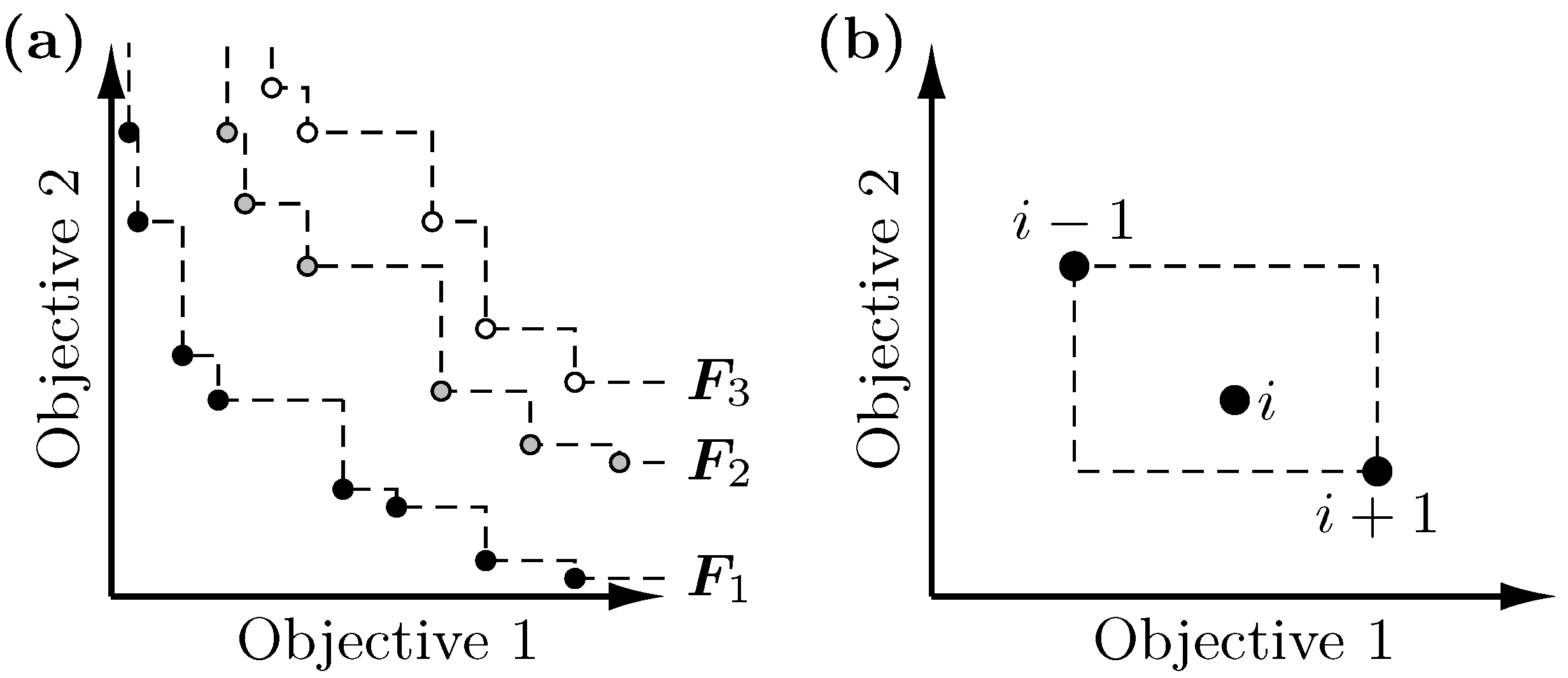
Figure 1 shows the two steps that NSGA-II uses to assign fitness. It is crucial to assign better fitness to members of the population that are not dominated by another member [
39]. In
Figure 1a it is shown how NSGA-II allocates every parent to a set (front)
, where
i is the rank of a solution. The Pareto front is
. The second front
is defined as the set of solutions that would be non-dominated if the Pareto front would have been removed from the offspring population. This allocation is repeated for
until all solutions are allocated to a front [
35]. Pareto elements have a rank of 1, members of
have rank 2 and so on. The efficient non-dominated sorting algorithm to allocate ranks is given in [
35].
Figure 1a shows the assignment of ranks for a set of solutions in objective space.
Figure 1b shows the concept of the crowding distance for a set of three solutions. It is a measure for the distribution density of solutions inside each front. For the
i-th solution it is determined by adding up the distances between its closed neighbors when sorted according to each objective. Preferring solutions with a larger crowding distance may lead to a more equally densely populated Pareto front. The solutions with minimum or maximum objective values are assigned an infinite crowding distance in order to preserve them [
35].
Rank and crowding distance make up the fitness function used in NSGA-II. In order to compare two solutions during tournament, the so-called crowded-comparison operator
is introduced. Its definition is as follows: A
B if the rank of A is lower than the rank of B. If both have equal ranks, A
B if the crowding distance of A is larger than B’s [
35].
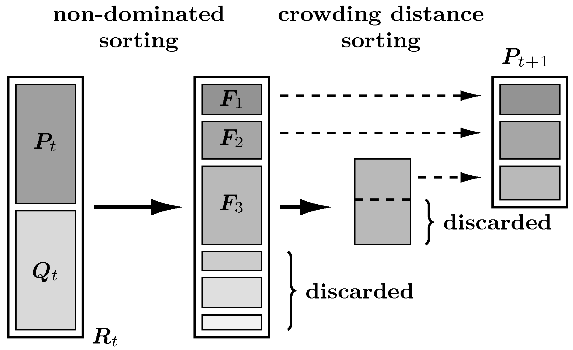
Figure 2 shows the procedure to generate a new parental generation
in NSGA-II after the first population is initialized randomly. From the parental population
an offspring population
is generated. Both populations are then merged into a combined population
in order to preserve the best solutions. All members of the combined population are then assigned ranks and crowding distances. The combined population is sorted according to the crowded-comparison operator and subsequently truncated to fit the defined population size by removing the less fit half of the population [
35]. Note that constraints are only considered during the generation of the offspring population
. Genes that violate constraints are less likely to be passed on. To ensure genetic diversity, members that violate constraints are not explicitly discarded during the generation of
.
3. Genotype-Phenotype Mapping
A multi-stage genotype-phenotype mapping is used to ensure feasible solutions and to decrease computational effort. The central idea behind this approach is to map the search-space to a so called solution space in a way that the size of the space is reduced and an additional constraint is introduced [
40,
41]. Even though there exists one parameter in the gene for every finite element in the structure, the gene is not directly used as a material distribution for the finite element solver. The binary gene is mapped to a finite element mesh by a multi-stage procedure acting as a further geometrical constraint to the optimization. This solution repair technique used as a constraint handling method is a comparable projection from the space of solutions to a subspace of feasible solutions [
42,
43]. A two-stage process to remove excess material is used for the design of 2D auxetic materials [
44].
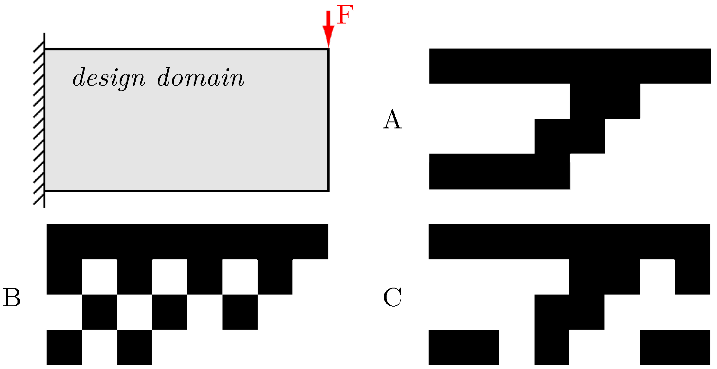
Figure 3 shows three binary solutions A, B and C to a simple design problem with a coarse discretization. B shows checkerboard structures and C shows arbitrary geometrical features and unconnected material floating in space. Both solutions are not feasible results for engineering purposes. A might be a more feasible design. Solution C performs considerably worse than A, however, it contains interesting geometrical features that should not be discarded or be assigned a bad fitness.
There are two ways to tackle the presented complications: instead of simply discarding C, its performance can be significantly improved by small changes in parameter space, and instead of accepting B as an optimal solution one might prefer solution A. Even though this means worse results in objective space, solution A is more near-net shape than the other two and is therefore better suited as a design recommendation. This means that for application both, parameter and objective space, cannot be viewed independently when evaluating multi-objective optimization results.
The above considerations show that unfeasible solutions must be avoided. In order to improve performance of the evolutionary algorithm one might want to not discard the solutions but to improve them. By the proposed genotype-phenotype mapping, several parameter combinations generated by genetic recombination and mutation are mapped to one feasible material distribution. The used problem-specific genotype-phenotype mapping is presented in detail in the following sections.
3.1. Feasibility Filtering
Solutions generated by probabilistic operators as in an evolutionary algorithm show arbitrary, noisy features. The goal of a topology optimization is to obtain organically smooth structures which we obtain by step-wise filling of holes and removal of outstanding material.
In order to be able to determine an element’s role inside the structure, it is necessary to obtain information about its surrounding. Initially, for every element inside the mesh a list of its neighboring elements (neighbors) is created. The binary encoding allows to easily classify any finite element as either solid or void. In order to avoid bias by the element numbering the filter is implemented such that the remove and fill operations are carried out cohesively after every step. Fixed elements are restored after every step that removes solid elements. As the filtering described in this section leads to structures that seem to be more feasible design suggestions for an engineer, the filtering will henceforth be referred to a as feasibility filtering.
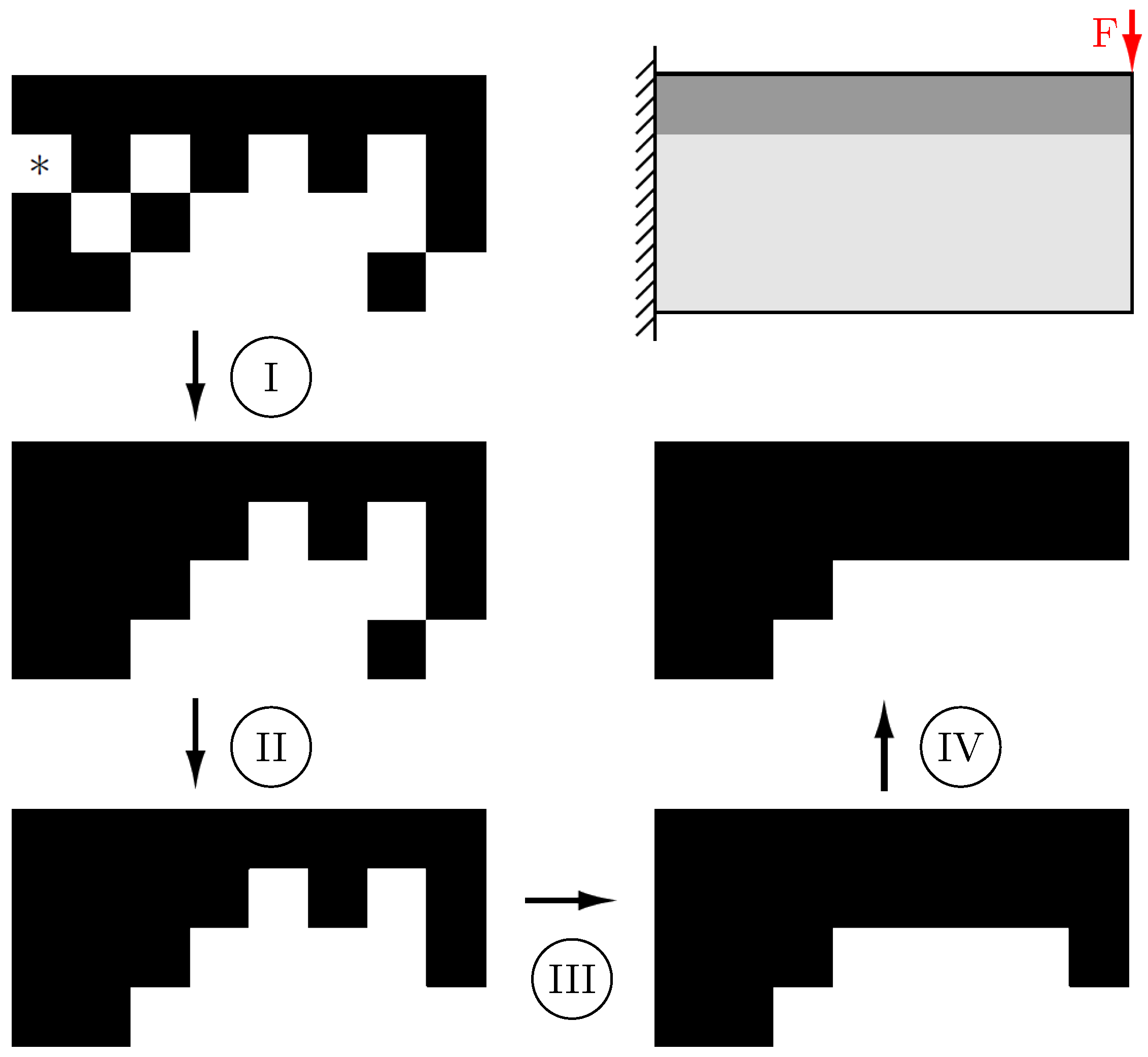
Figure 4 shows the consecutive steps of the filtering process. In the first step all void elements that are surrounded on all sides by solid elements are filled. Therefore, the number of solid neighbors is compared to the maximum number of neighbors counted earlier. An exception is made for elements to which boundary conditions were applied. Any surface with boundary conditions is treated as another solid neighbor. This ensures connection of the structure to applied loads and bearings. The following steps are similar to the first one. In the second step all solid elements that are not connected to another solid element over at least one surface are removed. Again, surfaces with boundary conditions are considered as a solid neighbor. The third and forth step fill holes that are surrounded by solid material on all but one side and remove solid elements that are connected to other elements over one side only, respectively. A fifth step (not shown in
Figure 4) is introduced for three-dimensional structures where void elements that are surrounded by four solid elements are filled.
3.2. Removal of Isolated Material
The solution to a mechanical design problem must be a single continuous body. Additional parts of unconnected material floating in space are observed when genes are generated by recombination and mutation. This isolated material leads to overestimation of the volume, which may result in underrating the fitness of a member. In order to obtain a light-weight, compact structure, all unconnected material must be removed. Here we describe an approach to remove material that is not connected to any fixed element.
Connections of solid elements to fixed domains are determined using a maze-solving strategy similar to Trémaux’s algorithm [
45]. The basic idea is that from any element inside the main structure there exists a continuous path through solid elements to a fixed element. If such a path does not exist, the elements are not connected to the main structure and can therefore be removed. The deterministic algorithm presented here will try all possible links. If it eventually reaches a fixed element all elements that were part of the path will be flagged as keep and will therefore not be removed. If all possible paths were tried and no fixed element was encountered, all elements in the path will be flagged delete. The algorithm starts at the lowest numbered solid element that is not fixed. After the first path is flagged either keep or delete, another starting point is to be determined. Again, the lowest numbered solid element without any flag is chosen and the procedure is repeated until either an element with a fixed or keep flag is encountered or a delete flag has to be set. The procedure ends when all solid elements are flagged. Subsequently, all parameters with a delete flag are set to 0 and therefore removed from the structure.
The algorithm to remove isolated material is depicted in Algorithm 1. A list of every element’s neighbors has been generated already for the feasibility filtering. Every element in the mesh is assigned a counter that is initialized to be the number of its solid neighbors. The paths are found by step-wise moving from an element to one of its neighbors. Every time the current position is changing to another element, that element is added to a set path and the counter of the element is lowered by 1. The neighbor to move to is the one that has the highest counter. If multiple elements share the highest counter, the one with the lowest element numbering is chosen. It is only possible to move to elements whose counter is not zero. If no neighbor fulfills this requirement anymore, all paths from that starting point have been tried and every element in the path set receives a delete flag.
| Algorithm 1 Removal of isolated material |
![Applmech 03 00080 i001]() |
3.3. Ground Element Filtering
Ground Element Filtering is a technique exploiting surface spline interpolation for projecting density distributions from a coarsely discretized mesh to another mesh of higher resolution [
46]. The coarse mesh is the parameter mesh that corresponds to the gene of a member and the finer finite element mesh will be used during the evaluation of the objective functions. The technique can be used to avoid checkerboard structures and to reduce the size of the gene. Even though the projection of a structure to a finer mesh does not improve the resolution of the structure, it does improve the results of the finite element analysis used as objective functions as it refines the spatial discretization [
47]. Furthermore, structures of elements only connected over their edge nodes are avoided, which is especially beneficial for thermal calculations. Using a coarse parameter mesh reduces the size of the gene and thus the computational effort of the optimization. The following description of the Ground Element Filtering process for binary density distributions is based on [
46,
48,
49]. Similar approaches are used with gradient based topology optimization strategies to ensure a binary distribution of the material density [
50,
51].
The parameter mesh consists of
m elements and the finer mesh consists of
elements. First, a real-valued density distribution
on the finer mesh is computed from the binary density distribution of the coarse mesh
as
where
is the Euclidean distance between two element’s volume centroids
. Centroids of elements of the finer mesh are indicated by an asterisk. A binary density distribution
is obtained by
with
.
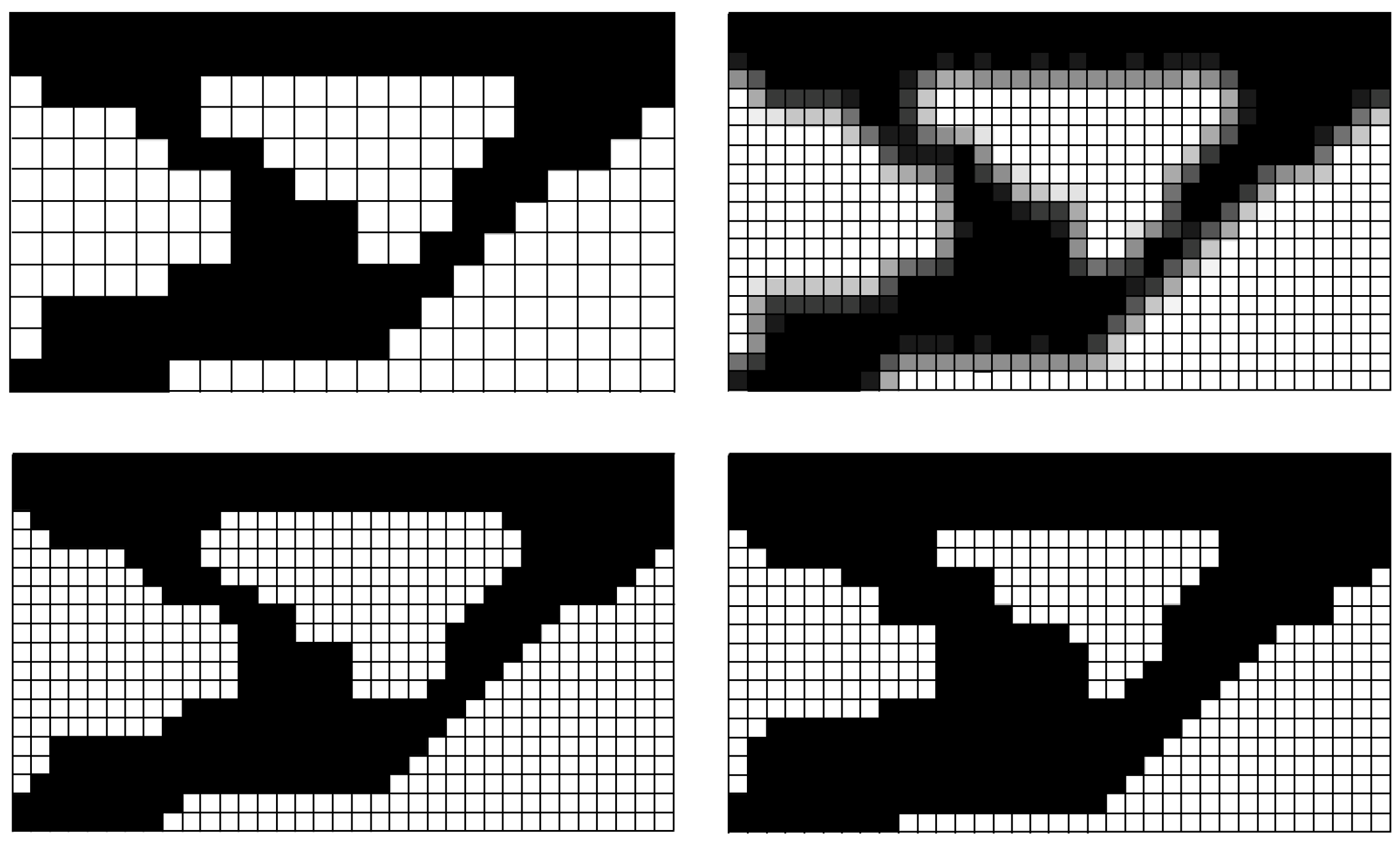
Figure 5 shows the real-value density distribution and two meshes with a binary distribution derived from a binary distribution on a coarse mesh. Higher values of
lead to a bulkier structure [
46]. Henceforth,
will be 0.4. This compensates for the fact that the feasibility filtering already generates bulkier structures as it forbids elements that are only connected to another element over their edge-nodes. In the presented genotype-phenotype mapping framework the Ground Element Filtering has two important tasks. The Ground Element Filtering ensures that resulting geometries are independent of anisotropies introduced by the choice of the base mesh. Any mesh can be mapped to another if they are bounded by the same surfaces. The two meshes do not have to be homogeneous and can consist of different elements. Ground Element Filtering also decouples the resolution of the structural features that are optimized from the mesh resolution required by the finite element solver.
As there is no a priori way to determine an adequate value of
, various preliminary tests may have to be conducted. This circumstance is tackled by the prior application of feasibilty filtering. In Equation (
2), it is necessary to invert an
matrix. Matrix inversion is computationally extensive due to high algorithmic complexity. This must be kept in mind when applying this method to large meshes.
3.4. Generation of a Structure from a Gene
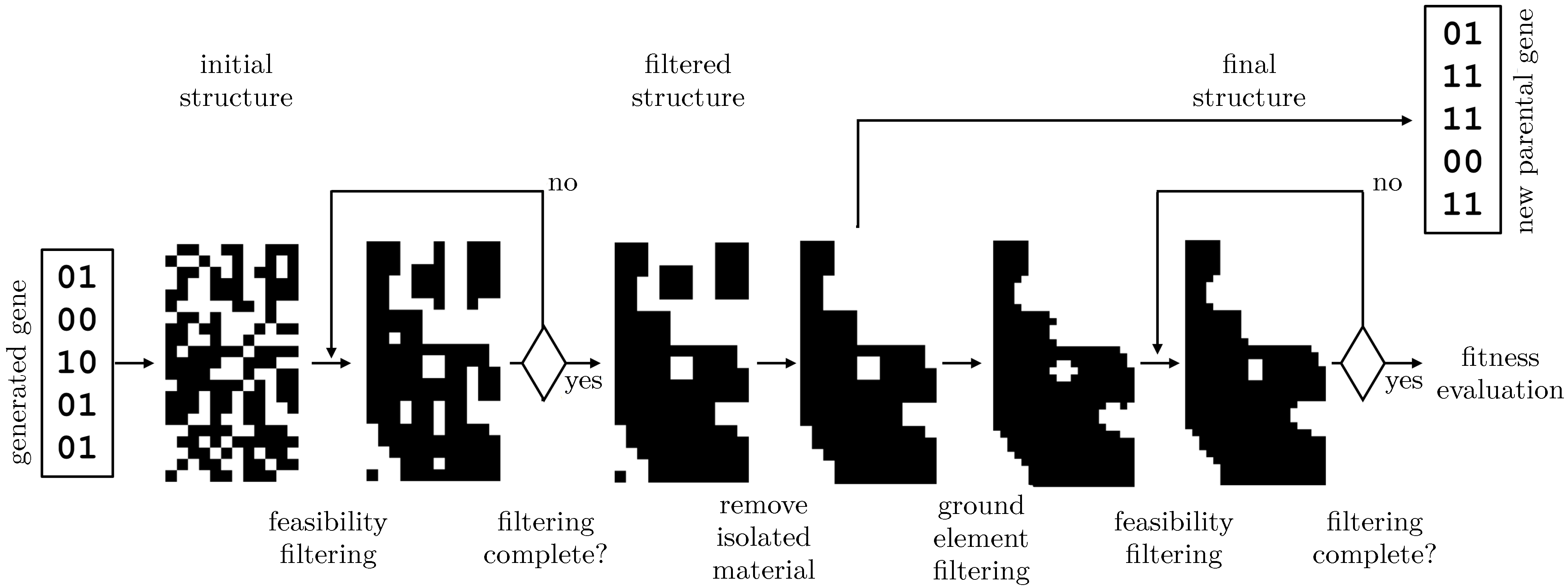
Figure 6 shows all stages of the genotype-phenotype mapping applied to a random parameter set. The feasibility filter is repeatedly applied to the coarse parameter mesh until the structure is no longer influenced by the filtering. This suppresses long outgrowths of material. Subsequently, isolated material is removed and Ground Element Filtering is used. Additional multi-stage feasibility filtering steps are applied to the fine finite element mesh in order to avoid artifacts from non-optimal Ground Element Filtering parameters. The application of the mapping is a strict geometric constraint to the optimization. The genotype-phenotype mapping generates a feasible structure from a gene and provides a binary element density distribution on a finite element mesh. The gene will be overwritten by the filtered structure before the Ground Element Filtering in order to pass on the feasible structure to subsequent generations rather than the initial noisy gene.
Note that the presented approach is not limited to use with NSGA-II or any evolutionary algorithm but can be applied whenever comparable problems are solved by probabilistic generation of binary density distributions. From the underlying finite element mesh and the binary density distribution, a 3D STL model can be derived for subsequent use in an engineering desing process.
4. Results
We define a design problem in terms of a geometric restriction (design domain) that is discretized by finite elements and load cases both mechanical and thermal. The load cases are defined by respective loads and boundary conditions. The objectives and constraints are functions of the calculated displacement, stress and temperature fields. All of the objective functions are chosen such that they are to be minimized. The relative volume
r is a further objective function. It is defined by the ratio of the volume of solid material to the volume of the design domain. For a homogeneous mass density
r is also the relative mass. All lengths are given in units of
L, stress is normalized by the elasticity modulus
E and temperature is normalized by
T. Elasticity and stationary thermal conduction are linear, so the absolute values of the loads do not influence the optimum shapes and are therefore not explicitly given. The Poisson’s ratio of the considered material is always 0.27. The population size was chosen to be higher than the number of parameter considered [
52] and the optimization was terminated after 100 generations without change in the Pareto front as there is no general abortion criterion for an evolutionary algorithm [
53].
From the last population all found non-dominated solutions that do not violate a constraint were chosen as feasible design propositions. The presented extensive genotype-phenotype mapping generates large, smooth meshes for the finite element solver. The objective functions are qualitative measures for the performance of the found solutions but still depend strongly on the resolution and surface quality of the generated finite element mesh. Quantitative results can be obtained by application of a smoothing procedure [
54] and subsequent remeshing with a higher resolution. The computational effort of such a procedure would be significantly higher and yet we expect no different solutions in parameter space by such a refined procedure.
4.1. Mechanical Two-Dimensional Problems
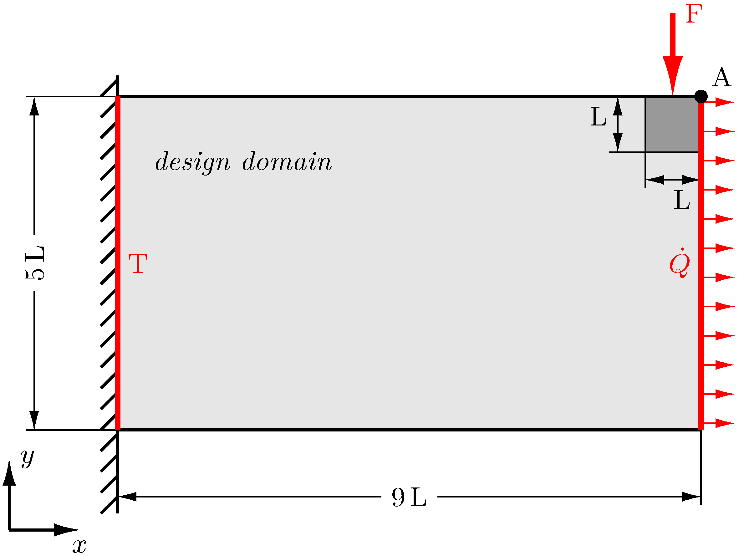
Figure 7 shows a rectangular beam design domain with mechanical and thermal loading conditions. The finite element mesh consists of 700 uniform elements and 243 binary parameters were used. Fixed elements are shaded and a point A is defined at which displacement and thermal boundary conditions are evaluated. The left side of the beam is fixed to the wall and on the right side a mechanical force
F is applied. On the wall the temperature
T is given and at the right side of the beam a uniform heat-flow
is cooling the beam.
Figure 8 shows sets of optimization results to the problem given in
Figure 7 in objective space after 120 generations with a population size of 300. Five sets were obtained each in independent runs with either full genotype-phenotype mapping enabled (blue) or only Ground Element Filtering enabled (red) to ensure comparability of the objective functions. The first objective function is the relative volume
r defined as
where
is the binary density distribution of the fine mesh and
is the volume of the
n-th finite element in the mesh. The second objective function is the absolute nodal displacement of point A in
y-direction
taken directly from the finite element calculation and normalized by the length
L. The relative volume was constraint to
and the maximum von Mises stress is restricted to be lower than 0.003
E. The maximum stress is evaluated among all elements with non-zero density and is also taken from the output of the finite element solver. To provide material-independent data the stress is normalized by the elastic modulus
E.
Both approaches show scattering of the approximated Pareto front typical for stochastic meta-heuristics in multi-objective optimization. The fronts are densely populated in every case and with respective to both objectives. Towards a larger relative volume the population density of the set rises. The number of non-dominated solutions that do not violate constraints is 30–55 with genotype-phenotype mapping and 14–43 without genotype-phenotype mapping enabled. The superior performance of the optimizer with enabled genotype-phenotype mapping is clearly visible when the dominance of the found solutions is compared. Apart from one single solution all solutions found with genotype-phenotype mapping enabled dominate the solutions found without genotype-phenotype mapping even though the parameter space is drastically reduced. The optimizer with disabled genotype-phenotype mapping was not able to find solutions with where as enabled genotype-phenotype mapping provides solutions in every run. The genotype-phenotype mapping lets the optimizer find more better perfoming solutions in a wider range of both objective functions.
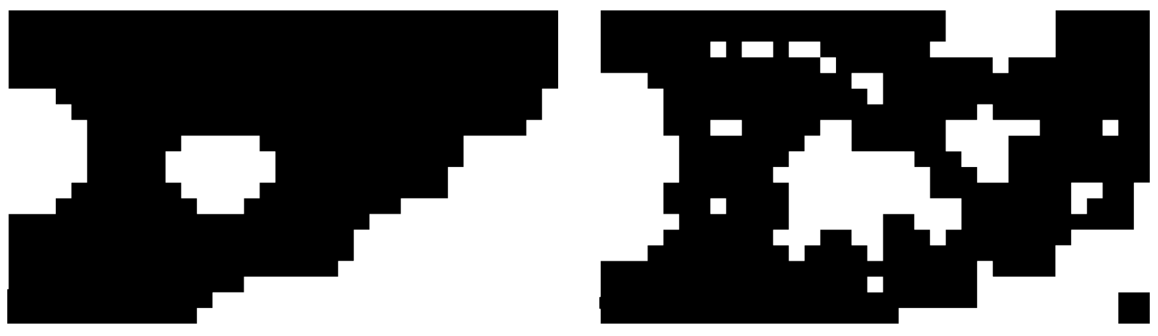
Figure 9 shows the influence of the genotype-phenotype mapping parameter space. Both presented solutions were members of an approximated Pareto front after 120 generations obtained in two independent optimization runs with a population size of 300. Both have a relative volume of 0.7. In one case the genotype-phenotype mapping was used as described in the previous section. During the other run the filtering procedure and the removal of isolated material was bypassed. Ground Element Filtering was used in both cases to ensure comparability of the two structures. The filtered structure shows smooth outlines and provides a feasible starting point for engineering design compared to the structure that was found without filtering. In the same time the presented mapping approach can accelerate the optimization procedure by effectively converting unfeasible solutions to a set of feasible solutions. An optimization approach without the genotype-phenotype mapping will require not only more generated members but also additional geometrical constraints to find comparably suited solutions.
The unfiltered structure is bulkier than the filtered one, even though it has the same relative volume. This is due to the many small holes that were generated. Moreover, some material is not connected to the beam, which leads to a wrong position of the solution in objective space. Both of these issues are addressed directly by the mapping. It may be possible to generate a smoother structure by a more fitting choice of , but there is no general method to determine this factor a priori. The filtering procedure described in this work diminishes the influence of poorly chosen while still benefiting from the advantages of the Ground Element Filtering. As the same computational effort is required to obtain the two presented structures the benefit of a specific genotype-phenotype mapping becomes apparent. We are able to obtain substantially better results in terms of engineering design application from the presented filtering technique with negligible additional effort.
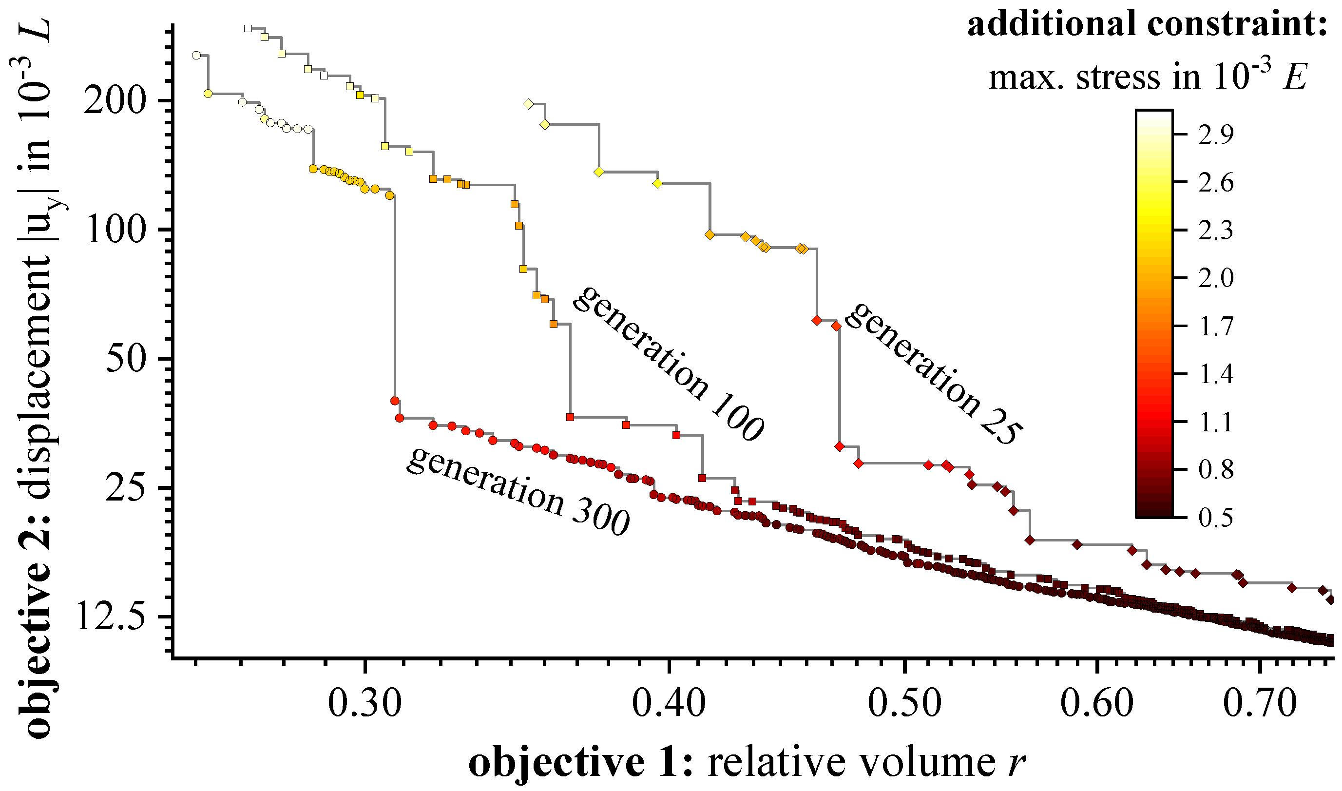
Figure 10 shows the temporal development of the found Pareto fronts. Given are the sets of obtained non-dominated solutions in objective space after 25, 100 and 300 generations. The additional stress constraint is indicated by colors. The population size is 300 and the sets consist of 36, 117 and 203 non-dominated members that do not violate any constraint, respectively.
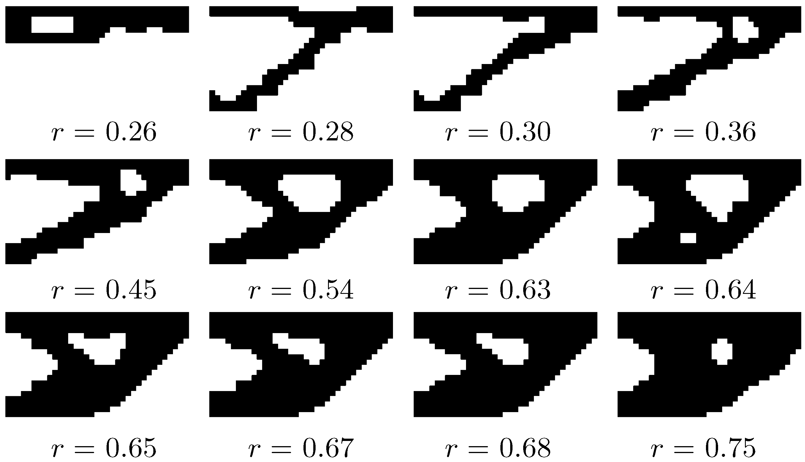
Figure 11 shows twelve optimized solutions to the design problem of
Figure 7. The solution are taken from a single front presented in
Figure 10 after 300 generations. The first solution with the least relative volume fundamentally distinguishes from the others because it is basically a horizontal beam with a lengthy hole close to the supporting wall. The next heavier solutions consist of a horizontal beam and a diagonal supporting beam. The fourth and fifth structure show a different topology and an additional support structure. The heaviest solutions are rather similar to each other and only the thickness of the structure seems to increase.
4.2. Thermo-Mechanical Problems
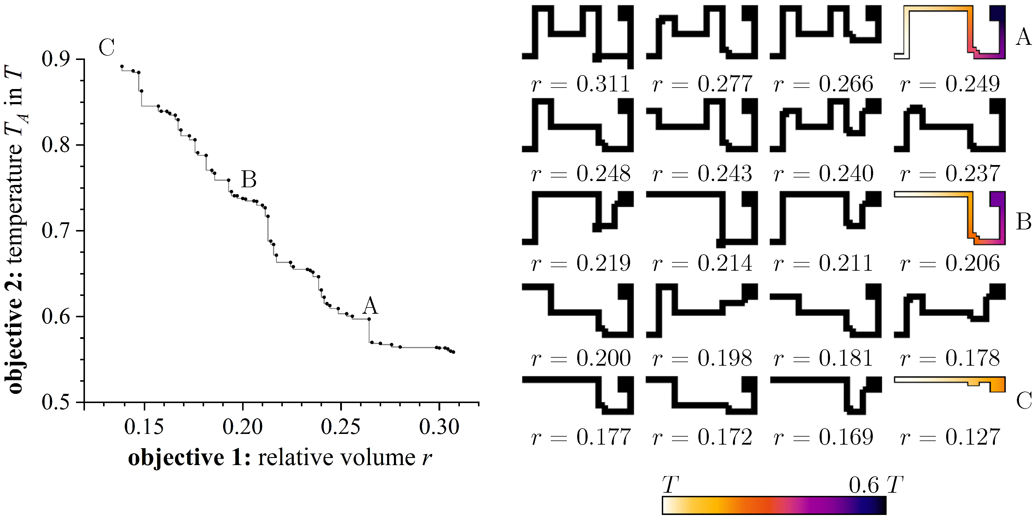
Figure 12 shows 20 solutions to the thermal design problem shown in
Figure 7 found after 1000 generations and with a population size of 300. The nodal temperature in point A and the relative volume
are to be minimized. The problem formulation can be interpreted as finding the optimal connecting structure between a heat drain and a surface that is to be cooled.
All found structures are thin lines that resemble printed circuit board tracks with a width of two elements. The lightest structure is a simple connection between the two surfaces. The structure with the lowest contact temperature is showing two distinct geometrical features. First, the whole heat drain is covered in material to maximize the heat transfer rate. The second feature is a meandering structure of the connection. All structures shown are path-shaped so the meandering leads to a longer path and thus the thermal resistance of the structure rises. Over the course of the Pareto set of solutions the meandering decreases in both amplitude and frequency while minimizing the volume. Single solutions show spots at which the width of the connection is more than two elements. This is probably due to a inadequately set Ground Element Filtering parameter . The structures seem circuit board-like because of the rectangular structures. No predominant diagonal structures were found in any of the optimized solutions. This is an indicator for an anisotropy caused by either the mesh or the genotype-phenotype mapping. Assuming no geometrical constraints, better performing solutions could have been found by carrying meandering even further. This is an example for solutions that converge towards a microstructure if meshes are continuously refined. The coarse parameter mesh imposes a geometrical constraint by setting a minimum size for any geometrical feature. In the present case this has a positive effect for application because it forces solutions to stay machinable.
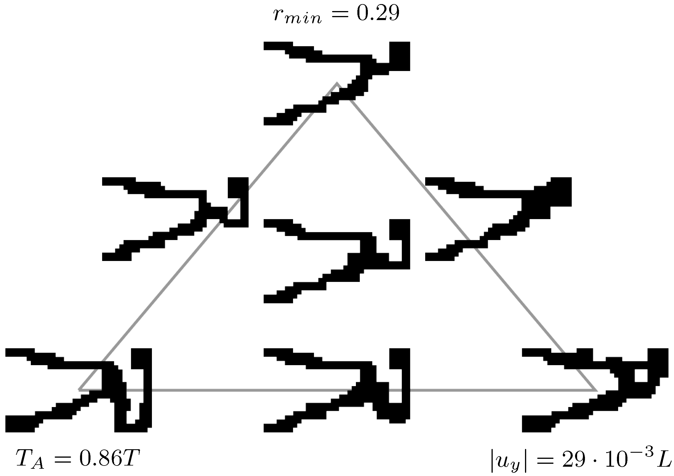
Figure 13 shows seven solutions to the design problem shown in
Figure 7 found after 1000 generations and with a population size of 300. The contact temperature and displacement in point
A as well as the relative volume
are to be minimized. The maximum von Mises stress is restricted to
and the displacement is restricted to
. This is an optimization with respect to three objective functions and three constraints in two load cases.
The presented solutions represent single-objective optima, trade-offs between the single-objective optima and a trade-off between all three objectives. Analogous to the results in
Figure 12, one can see that, in order to minimize the contact temperature, meandering structures and full contact with the right edge are favorable. The structure itself distinguishes significantly from the results presented in
Figure 12 because multiple mechanical constraints are to be taken into account. The stiffest solution resembles the solutions presented in
Figure 11, but no similar solution was found because another constraint is imposed.
From this set of optimized results it is possible to obtain information about what geometrical features influence the objectives. The trade-off solutions presented in
Figure 13 illustrate that the geometrical feature’s influence decreases when the importance of another objective is increased.
4.3. Mechanical Three-Dimensional Problems
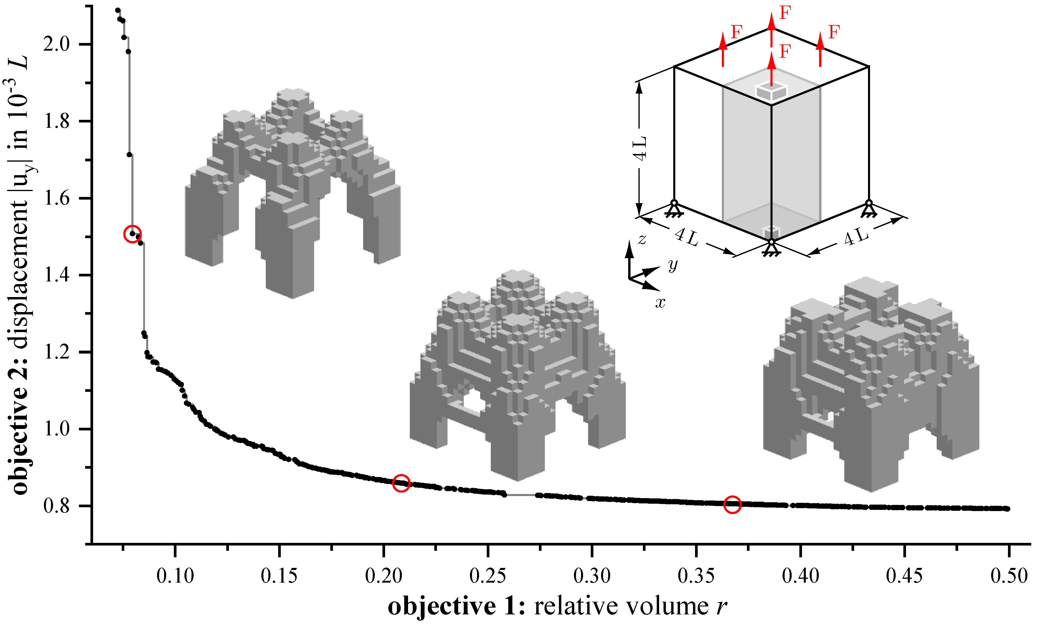
Figure 14 shows a three-dimensional design problem with three optimized results. The design domain is a cube with four of its edges fixed and four point loads
F on the opposite side of the cube [
55]. Due to this symmetry, the design domain is chosen to be only one fourth of the cube with fixed elements at the load sites and at the fixed points. Objectives are the displacement at the loading site and the relative volume
. The maximum stress is constraint to be
. The finite element mesh consists of 2000 uniform elements and the gene consists of 427 bits. This is the largest structure optimized in this work. The symmetric loading conditions will disclose spurious anisotropies of the optimization procedure.
The optimum structure for this design problem is described as a quadropod solution with solid legs transferring the point loads to the nearest supports and additional material interconnecting the legs that was obtained on a mesh of
elements [
55]. This was not a multi-objective optimization. However, similar results were obtained by NSGA-II. Four leg-like connections between the fixed elements and interconnecting material between neighboring legs can be observed with the interconnections being in the upper part of the design space. Over the whole permitted range of
r, changes of the structures mostly consist of further thickening of the structure and larger interconnections.
The cubic design domain holds further symmetries that were not exploited. The three presented structures show a somewhat additional symmetry that was not a priori imposed to the system. This is an indicator for solutions close to optimal structures. When talking about additional unprescribed symmetries and similar shapes, one has to keep in mind the characteristics of the evolutionary optimizer used. Due to the probabilistic generation of the parameters slight unevenness can hardly be avoided.
5. Discussion
One might argue that the presented filtering procedure leads to loss of randomness or reduced diversity of the population, effects that are detrimental to any evolutionary algorithm. In the scope of this work we were always able to find extensive sets of non-dominated solutions with a densely populated Pareto front. The stability of NSGA-IIand the careful consideration of constraints in the presented optimization scheme is sufficient to find solutions close to the global optima even with such a strong additional constraint as the presented genotype-phenotype mapping. For all results given in this work the population size and number of generations were chosen near to the acceptable minimum.
The implementation of the feasibility filtering of course implies a priori knowledge of engineering design with linear elasticity and stationary heat conduction. The filtering procedure presented here is not universal with respect to physical effects that might be considered. For example, long outgrowth of material is very advantageous once surface effects, such as convection, come into play. This is a mere demonstration of the capability of a specific genotype-phenotype mapping for topology optimization in engineering design.
The optimization scheme presented in this work offers the potential to provide insights in the complex relationship between structural features and feasibility for engineering application. It can be understood as a first step in computer aided design and that results in deeper understanding of the tackled design problem. Dense sets of near-optimum design propositions considering multiple objectives and constraints derived from different physical models are found. The presented method has potential in application way beyond the discussed matter of this work. The optimization scheme itself is not limited to three objectives and constraints. However, there might be approaches that are more suited for a larger number of objectives.
6. Conclusions
We developed a tool for multi-objective topology optimization using the evolutionary algorithm NSGA-II. A specific genotype-phenotype mapping ensures optimized structures to be of practical value for engineering design. Probabilistically generated binary material distributions are iteratively smoothed, isolated material is removed and the structure is projected on a finer mesh.
We find dense sets of optimized solutions considering three independent objectives and three additional constraints without a priori definition of objective weighting schemes. Evaluation of objectives and constraints are based on linear elastic deformation and stationary heat transfer calculations. Structures with up to 2000 design variables were optimized.
The described genotype-phenotype mapping effectively avoids checkerboard structures and ensures feasibility of the generated structures. Anisotropy due to the underlying discretization of the design space is reduced when the discretization is chosen appropriately.
The filtering procedure efficiently improves unfeasible structures while not diminishing the crucial genetic diversity, leading to significantly improved performance. The proposed methodology allows to find dense sets of feasible design proposition with no further assumptions about their position in objective space. The basic methodology is not limited to the number of objectives and constraints used in this work.
The presented optimization procedure is beneficial for engineering design as an early-stage tool. Sets of Pareto solutions found during optimization provide detailed insights into the relation between distinct geometrical features and performance in objective space.
Author Contributions
Conceptualization, F.S. and K.D.; methodology, F.S.; software, F.S. and K.D.; validation, F.S.; formal analysis, F.S.; investigation, F.S.; resources, F.S. and K.D.; writing—original draft preparation, F.S.; writing—review and editing, F.S. and K.D.; visualization, F.S.; supervision, K.D.; project administration, K.D.; funding acquisition, K.D. All authors have read and agreed to the published version of the manuscript.
Funding
This work was funded by the European Union via the European Regional Development Fund (ERDF).
Data Availability Statement
The open source finite element code is available at
https://en.z88.de/download-z88os/ (accessed on 1 November 2022). The optimization code and data are available from the corresponding author on reasonable request.
Conflicts of Interest
The authors declare that they have no conflict of interest.
Abbreviations
The following abbreviations are used in this manuscript:
| NSGA-II | Non-Sorting Genetic Algorithm II |
References
- Bendsøe, M.P.; Kikuchi, N. Generating optimal topologies in structural design using a homogenization method. Comput. Methods Appl. Mech. Eng. 1988, 71, 197–224. [Google Scholar] [CrossRef]
- Bendsøe, M.P. Optimal shape design as a material distribution problem. Struct. Optim. 1989, 1, 193–202. [Google Scholar] [CrossRef]
- Eschenauer, H.A.; Olhoff, N. Topology Optimization of Continuum Structures: A Review. Appl. Mech. Rev. 2001, 54, 331–390. [Google Scholar] [CrossRef]
- Bendsøe, M.P.; Sigmund, O. Topology Optimization: Theory, Methods, and Applications, 2nd ed.; Springer: Berlin/Heidelberg, Germany, 2004. [Google Scholar]
- Sigmund, O.; Petersson, J. Numerical Instabilities in Topology Optimization: A Survey on Procedures Sealing with Checkerboards, Mesh-dependencies and Local Minima. Struct. Multidiscip. Optim. 1998, 16, 68–75. [Google Scholar] [CrossRef]
- Aage, N.; Andreassen, E.; Lazarov, B.S.; Sigmund, O. Giga-voxel computational morphogenesis for structural design. Nature 2017, 550, 84–86. [Google Scholar] [CrossRef] [Green Version]
- Suzuki, K.; Kikuchi, N. A homogenization method for shape and topology optimization. Comput. Methods Appl. Mech. Eng. 1991, 93, 291–318. [Google Scholar] [CrossRef] [Green Version]
- Wang, L.; Zhao, X.; Liu, D. Size-controlled cross-scale robust topology optimization based on adaptive subinterval dimension-wise method considering interval uncertainties. Eng. Comput. 2022, 38, 5321–5338. [Google Scholar] [CrossRef]
- Wang, L.; Liu, Y.; Li, M. Time-dependent reliability-based optimization for structural-topological configuration design under convex-bounded uncertain modeling. Reliab. Eng. Syst. Saf. 2022, 221, 108361. [Google Scholar] [CrossRef]
- Li, Z.; Wang, L.; Luo, Z. A feature-driven robust topology optimization strategy considering movable non-design domain and complex uncertainty. Comput. Methods Appl. Mech. Eng. 2022, 401, 115658. [Google Scholar] [CrossRef]
- Wang, L.; Liu, Y.; Wang, X.; Qiu, Z. Convexity-oriented reliability-based topology optimization (CRBTO) in the time domain using the equivalent static loads method. Aerosp. Sci. Technol. 2022, 123, 107490. [Google Scholar] [CrossRef]
- Obayashi, S.; Sasaki, D. Self-organizing map of pareto solutions obtained from multiobjective supersonic wing design. In Proceedings of the 40th AIAA Aerospace Sciences Meeting & Exhibit, Reno, NV, USA, 14–17 January 2002; p. 991. [Google Scholar]
- Branke, J. (Ed.) Multiobjective Optimization: Interactive and Evolutionary Approaches; Springer: Berlin, Germany, 2008. [Google Scholar]
- Oyama, A.; Nonomura, T.; Fujii, K. Data mining of Pareto-optimal transonic airfoil shapes using proper orthogonal decomposition. J. Aircr. 2010, 47, 1756–1762. [Google Scholar] [CrossRef]
- Miettinen, K. Nonlinear Multiobjective Optimization; Springer Science & Business Media: Cham, Switzerland, 2012; Volume 12. [Google Scholar]
- Deb, K.; Sindhya, K.; Hakanen, J. Multi-objective optimization. In Decision Sciences; Sengupta, R.N., Gupta, A., Dutta, J., Eds.; CRC Press: Boca Raton, FL, USA, 2016. [Google Scholar]
- Koski, J. Multicriteria truss optimization. In Multicriteria Optimization in Engineering and in the Sciences; Springer: Cham, Switzerland, 1988; pp. 263–307. [Google Scholar]
- Das, I.; Dennis, J.E. Normal-boundary intersection: A new method for generating the Pareto surface in nonlinear multicriteria optimization problems. SIAM J. Optim. 1998, 8, 631–657. [Google Scholar] [CrossRef] [Green Version]
- Messac, A.; Ismail-Yahaya, A.; Mattson, C.A. The normalized normal constraint method for generating the Pareto frontier. Struct. Multidiscip. Optim. 2003, 25, 86–98. [Google Scholar] [CrossRef]
- Sato, Y.; Izui, K.; Yamada, T.; Nishiwaki, S. Pareto frontier exploration in multiobjective topology optimization using adaptive weighting and point selection schemes. Struct. Multidiscip. Optim. 2017, 55, 409–422. [Google Scholar] [CrossRef]
- Sato, Y.; Yaji, K.; Izui, K.; Yamada, T.; Nishiwaki, S. Topology optimization of a no-moving-part valve incorporating Pareto frontier exploration. Struct. Multidiscip. Optim. 2017, 56, 839–851. [Google Scholar] [CrossRef]
- Sato, Y.; Yaji, K.; Izui, K.; Yamada, T.; Nishiwaki, S. An optimum design method for a thermal-fluid device incorporating multiobjective topology optimization with an adaptive weighting scheme. J. Mech. Des. 2018, 140, 031402. [Google Scholar] [CrossRef]
- Doi, S.; Sasaki, H.; Igarashi, H. Multi-objective topology optimization of rotating machines using deep learning. IEEE Trans. Magn. 2019, 55, 7202605. [Google Scholar] [CrossRef]
- Guirguis, D.; Hamza, K.; Aly, M.; Hegazi, H.; Saitou, K. Multi-objective topology optimization of multi-component continuum structures via a Kriging-interpolated level set approach. Struct. Multidiscip. Optim. 2015, 51, 733–748. [Google Scholar] [CrossRef]
- Lim, J.; You, C.; Dayyani, I. Multi-objective topology optimization and structural analysis of periodic spaceframe structures. Mater. Des. 2020, 190, 108552. [Google Scholar] [CrossRef]
- Deb, K.; Goel, T. A hybrid multi-objective evolutionary approach to engineering shape design. In Proceedings of the International Conference on Evolutionary Multi-Criterion Optimization, Zurich, Switzerland, 7–9 March 2001; Springer: Cham, Swizterland, 2001; pp. 385–399. [Google Scholar]
- Aguilar Madeira, J.F.; Rodrigues, H.; Pina, H. Multi-Objective Optimization of Structures Topology by Genetic Algorithms. Adv. Eng. Software 2005, 36, 21–28. [Google Scholar] [CrossRef]
- Kunakote, T.; Bureerat, S. Multi-Objective Topology Optimization using Evolutionary Algorithms. Eng. Optim. 2011, 43, 541–557. [Google Scholar] [CrossRef]
- Peña, S.I.V.; Rionda, S.B.; Aguirre, A.H. Multiobjective Shape Optimization Using Estimation Distribution Algorithms and Correlated Information. In Proceedings of the International Conference on Evolutionary Multi-Criterion Optimization, Guanajuato, Mexico, 9–11 March 2005; Springer: Cham, Swizterland, 2005; pp. 664–676. [Google Scholar]
- Bureerat, S.; Srisomporn, S. Optimum Plate-Fin Heat Sinks by using a Multi-Objective Evolutionary Algorithm. Eng. Optim. 2010, 42, 305–323. [Google Scholar] [CrossRef]
- Kanyakam, S.; Bureerat, S. Multiobjective Optimization of a Pin-Fin Heat Sink Using Evolutionary Algorithms. J. Electron. Packag. 2012, 134, 021008. [Google Scholar] [CrossRef]
- Kanyakam, S.; Bureerat, S. Multiobjective Evolutionary Optimization of Splayed Pin-Fin Heat Sink. Eng. Appl. Comput. Fluid Mech. 2014, 5, 553–565. [Google Scholar] [CrossRef] [Green Version]
- Tai, K.; Prasad, J. Target-matching test problem for multiobjective topology optimization using genetic algorithms. Struct. Multidiscip. Optim. 2007, 34, 333–345. [Google Scholar] [CrossRef]
- Cardillo, A.; Cascini, G.; Frillici, F.S.; Rotini, F. Multi-objective topology optimization through GA-based hybridization of partial solutions. Eng. Comput. 2013, 29, 287–306. [Google Scholar] [CrossRef]
- Deb, K.; Pratap, A.; Agarwal, S.; Meyarivan, T. A Fast and Elitist Multiobjective Genetic Algorithm: NSGA-II. IEEE Trans. Evol. Comput. 2002, 6, 182–197. [Google Scholar] [CrossRef] [Green Version]
- Sigmund, O. On the usefulness of non-gradient approaches in topology optimization. Struct. Multidiscip. Optim. 2011, 43, 589–596. [Google Scholar] [CrossRef]
- Mitchell, M. An Introduction to Genetic Algorithms; MIT Press: Cambridge, MA, USA, 2001. [Google Scholar]
- Harvey, I. Artificial Evolution: A Continuing SAGA. Lect. Notes Comput. Sci. 2001, 2217, 94–109. [Google Scholar]
- Zitzler, E.; Thiele, L. Multiobjective Evolutionary Algorithms: A Comparative Case Study and the Strength Pareto Approach. IEEE Trans. Evol. Comput. 1999, 3, 257–271. [Google Scholar] [CrossRef] [Green Version]
- Banzhaf, W. Genotype-phenotype-mapping and neutral variation—A case study in genetic programming. In Proceedings of the International Conference on Parallel Problem Solving from Nature, Jerusalem, Israel, 8–14 October 1994; Springer: Cham, Switzerland, 1994; pp. 322–332. [Google Scholar]
- Keller, R.E.; Banzhaf, W. Genetic programming using genotype-phenotype mapping from linear genomes into linear phenotypes. In Proceedings of the 1st Annual Conference on Genetic Programming, Stanford, CA, USA, 28–31 July 1996; MIT Press: Cambridge, MA, USA, 1996; pp. 116–122. [Google Scholar]
- Salcedo-Sanz, S. A survey of repair methods used as constraint handling techniques in evolutionary algorithms. Comput. Sci. Rev. 2009, 3, 175–192. [Google Scholar] [CrossRef]
- Krawiec, K. Metaheuristic design pattern: Candidate solution repair. In Proceedings of the Companion Publication of the 2014 Annual Conference on Genetic and Evolutionary Computation, Vancouver, BC, Canada, 12–16 July 2014; pp. 1415–1418. [Google Scholar]
- Borovinšek, M.; Novak, N.; Vesenjak, M.; Ren, Z.; Ulbin, M. Designing 2D auxetic structures using multi-objective topology optimization. Mater. Sci. Eng. A 2020, 795, 139914. [Google Scholar] [CrossRef]
- Even, S.; Even, G.; Karp, R.M. (Eds.) Graph Algorithms, 2nd ed.; Cambridge University Press: Cambridge, UK, 2012. [Google Scholar]
- Bureerat, S.; Limtragool, J. Structural Topology Optimisation using Simulated Annealing with Multiresolution Design Variables. Finite Elem. Anal. Des. 2008, 44, 738–747. [Google Scholar] [CrossRef]
- Fenner, R.T. Finite Element Methods for Engineers, 2nd ed.; Imperial College Press: London, UK, 2013. [Google Scholar]
- Bureerat, S.; Boonapan, A.; Kunakote, T.; Limtragool, J. Design of Compliance Mechanisms using Topology Optimisation. In Proceedings of the 19th Conference of Mechanical Engineering Network of Thailand, Phuket, Thailand, 19–21 October 2005; pp. 421–427. [Google Scholar]
- Bureerat, S.; Limtragool, J. Performance Enhancement of Evolutionary Search for Structural Topology Optimisation. Finite Elem. Anal. Des. 2006, 42, 547–566. [Google Scholar] [CrossRef]
- Guest, J.K. Topology optimization with multiple phase projection. Comput. Methods Appl. Mech. Eng. 2009, 199, 123–135. [Google Scholar] [CrossRef]
- Wang, F.; Lazarov, B.S.; Sigmund, O. On projection methods, convergence and robust formulations in topology optimization. Struct. Multidiscip. Optim. 2011, 43, 767–784. [Google Scholar] [CrossRef]
- Alander, J.T. On Optimal Population Size of Genetic Algorithms. In Proceedings of the Comp Euro ’92. Computer Systems and Software Engineering, Hague, The Netherlands, 4–8 May 1992; pp. 65–70. [Google Scholar]
- Sigmund, O.; Maute, K. Topology Optimization Approaches. Struct. Multidiscip. Optim. 2013, 6, 1031–1055. [Google Scholar] [CrossRef]
- Deese, K.; Geilen, M.; Rieg, F. A Two-step Smoothing Algorithm for an Automated Product Development Process. Int. J. Simul. Model. (IJSIMM) 2018, 17, 308–317. [Google Scholar] [CrossRef]
- Olhoff, N.; Ronholt, E.; Scheel, J. Topology Optimization of Three-Dimensional Structures using Optimum Microstructures. Struct. Optim. 1998, 16, 1–18. [Google Scholar] [CrossRef]
| Publisher’s Note: MDPI stays neutral with regard to jurisdictional claims in published maps and institutional affiliations. |
© 2022 by the authors. Licensee MDPI, Basel, Switzerland. This article is an open access article distributed under the terms and conditions of the Creative Commons Attribution (CC BY) license (https://creativecommons.org/licenses/by/4.0/).


