Article

On the Countering of Free Vibrations by Forcing: Part I—Non-Resonant and Resonant Forcing with Phase Shifts

by
Luiz M. B. C. Campos
and
Manuel J. S. Silva
*,†
CCTAE, IDMEC, LAETA, Instituto Superior Técnico, Universidade de Lisboa, Av. Rovisco Pais 1, 1049-001 Lisboa, Portugal
*
Author to whom correspondence should be addressed.
These authors contributed equally to this work.
Appl. Mech. 2022, 3(4), 1352-1384; https://doi.org/10.3390/applmech3040078
Submission received: 29 September 2022 / Revised: 23 November 2022 / Accepted: 29 November 2022 / Published: 3 December 2022
(This article belongs to the Special Issue Feature Papers in Applied Mechanics)

Abstract

:
The question addressed is whether the free oscillations of a continuous system can be suppressed, or at least the total energy reduced, by applying external forces, using as example the linear undamped transverse oscillations of a uniform elastic string. The non-resonant forcing at an applied frequency, distinct from all natural frequencies, does not interact with the normal modes, whose energy is unchanged, and adds the energy of the forced oscillation, thus increasing the total energy, that is the opposite of the result being sought. The resonant forcing at an applied frequency, equal to one of the natural frequencies, leads to an amplitude growing linearly with time, and hence the energy is growing quadratically with time, implying an increase in total energy after a sufficiently long time. A reduction in total energy is possible over a short time, say over the first period of oscillation, by optimizing the forcing. In the case of a concentrated force, by optimizing its magnitude and location, the total energy with forcing in one period is reduced by a modest maximum of 2% relative to the free oscillation alone. The conclusion is similar for several concentrated forces. In the case of a continuously distributed force, by optimizing the spatial distribution, it is possible to reduce the energy of the total oscillation to one-fourth of that of the free oscillation over the first period of vibration. This shows that continuously distributed forces are more effective at vibration suppression than point forces.

1. Introduction

The research in the present paper relates to the active suppression of (a) acoustic oscillations and (b) vibrations of beams. Concerning the first topic (a) of acoustic oscillations, the simplest one-dimensional case is the classical problem of sound propagation in ducts [1,2,3,4,5,6,7], including active noise reduction [8,9]. The extensions include the acoustics of ducts of generally varying cross-section that is studied most simply for quasi-one-dimensional propagation [10,11,12], when the wavelength is larger than the transverse dimensions of the duct; in this case, the classical wave equation is replaced by the horn wave equation, for which a variety of solutions exist [13,14,15,16,17,18,19,20,21,22,23,24]. An extension including mean flow is the quasi-one-dimensional propagation of sound in a duct of varying cross-section [25,26,27,28,29,30,31]. A different extension, without flow, is the acoustics of curved [32,33,34,35,36,37,38,39,40,41,42,43,44,45,46,47] or twisted [48] tubes. The applications of duct acoustics include the noise of jet engines and air conditioning systems.
The topic (b) of vibration of beams is based on the classic Bernoulli [49] and Euler [50] theory that is a standard introductory subject in textbooks on elasticity [51,52,53,54,55,56,57,58,59] and leads to the phenomenon of buckling [60], which has been considered in several conditions: (i) geometric and material non-linearities [61,62]; (ii) in combination with shear [63,64] that is more significant for thin-walled beams [65,66,67,68,69]; (iii) constraints [70,71,72], such as hyper or non-local elasticity [73,74]; (iv) vibrations [75,76], that can be excited by unsteady applied forces [77,78,79,80,81,82,83], leading to control problems [84]; (v) steady mechanical [85] or thermal [86,87,88] effects; and (vi) vibrations of tapered beams [89,90,91,92,93,94,95,96,97,98,99,100,101,102,103,104,105], with multiple applications like airplane wings and flexible aircraft and helicopters [106,107,108,109,110,111,112,113,114,115]. The applications include active vibration suppression [116,117,118,119,120].
There are generic topics applicable to active vibration suppression [121] independent of specific application. The active suppression of (a) noise is based on (A) boundary or radiation conditions introducing sound waves with opposite phase. The active suppression (b) of vibration of beams is based on (B) forcing by applied forces and/or moments either concentrated or continuously distributed or a superposition of both. The contrast between the two approaches suggests an hybrid case concerning the active suppression of transverse oscillations of an elastic string, instead of (A) superimposing oscillations with opposite phase through the boundary using (B) forcing by concentrated or distributed forces. The hybrid case is investigated by considering whether the energy of free transverse oscillations of an elastic string can be reduced by forcing. The ( α ) undamped and ( β ) damped cases are described by different equations, namely the ( α ) classical wave equation and ( β ) the wave-diffusion or telegraph equation. This suggests considering ( α ) the undamped case first in the present paper (part I) to assess the interaction of free and forced oscillations, including non-resonant and resonant cases; the additional effects of damping ( β ) are considered in a follow-on paper (part II).
Thus the transverse oscillations of an elastic string are used as a sample case on the use of forcing for active suppression of material vibration. There are two cases to be considered [122], depending on whether the forcing is (II) or not (I) at a natural frequency of the undamped system. Assuming the free oscillation of the system, at its natural frequency (or frequencies), the forcing at any other, non-resonant frequency (case I) will increase the total energy, because the energy of the forced vibration adds to that of the free vibration. Thus, no vibration suppression will occur, unless forcing is applied at the natural frequency, leading to the resonant case (case II). Concerning the remaining second case (case II), with resonance: (i) the free oscillations are sinusoidal, with constant amplitude; (ii) the forced resonant oscillation is sinusoidal with amplitude increasing linearly with time; (iii) the total, free plus forced, oscillation, has amplitude varying with time. It is clear that the oscillation cannot be totally suppressed, and the total energy will eventually increase. Thus, the question can be modified: for how long can the energy of oscillation of an undamped system be prevented from increasing by optimizing the resonant forcing relative to the free oscillation? This is the basic question addressed in the present paper.
In this introduction, different problems have been identified by distinct symbols: (i) acoustic oscillations (a) and vibrations of beams (b); (ii) active partial or total suppression introducing opposite oscillations from sources or through the boundaries (A) or by forcing with applied forces and moments (B); (iii) models without ( α ) and with ( β ) damping; (iv) cases of non-resonant (I) or resonant (II) forcing. An additional criterion (v) would be forcing by point or continuous forces. With this classification, the part I of the paper concerns the transverse oscillations of an elastic string (a), forced by point or continuous forces (B), including non-resonant (I) and resonant (II) cases, without damping ( α ), with damping ( β ) being deferred to part II. The applications are undamped systems described by the classical wave equation (part I) and damped systems described by the wave-diffusion or telegraph equation (part II). The wave equation applies to acoustic, elastic and electromagnetic waves, and damping effects can be thermal conduction or radiation, viscosity, electrical resistance and mass diffusion. The theory of oscillations applies not only to continuous systems, but also to discrete systems such as: (i) mechanical oscillators consisting of masses, springs, dampers and forcing actuators; (ii) electrical circuits consisting of inductors, capacitors and resistors powered by batteries; (iii) analogous circuits in acoustics, hydraulics and other fields.
The question of vibration suppression is answered by an exact, analytical solution, for the “simplest” vibrating system and forcing: (i) the transverse vibrations of an elastic string fixed at both ends; (ii) resonant forcing by a single or several concentrated forces or a distributed force; (iii) minimization of the energy over the first period of oscillation. After outlining the problem (Section 1), the method of solution is presented as follows: calculation of the free oscillations, as a superposition of natural modes, and of the response to a concentrated force, in non-resonant cases (Section 2); calculation of the total (kinetic plus elastic) energy density, averaged over a period, for free, forced and combined oscillations (Section 3), showing that the energy adds in the non-resonant case, but not in the resonant case; thus, the energy integrated over the length of the string can be minimized with regard to the magnitude of the force, to the position where it is applied or both simultaneously (Section 4). In this way, the total energy can be reduced marginally (by less 2%), by optimum forcing, over the first period, but not much longer, as shown (Section 5) by plotting the total oscillation and its energy over a period for optimal and non-optimal forcing conditions. The case of several concentrated forces at different locations is equivalent to a single overall force and location (Section 6), and leads to the same result. In the case of a continuously distributed force (Section 7), it is shown that it is possible to reduce the total energy of the oscillation over the first period by to at best one-fourth of the energy of the free oscillation. This requires an optimal choice of the forcing, as concerns spatial distribution and amplitude relative to the free oscillation, and shows (Section 8) that continuously distributed forces are more effective vibration suppressors than point forces.
This kind of analysis could be applied to more general vibrating systems [1,2,3,4,5,6,7,123,124].

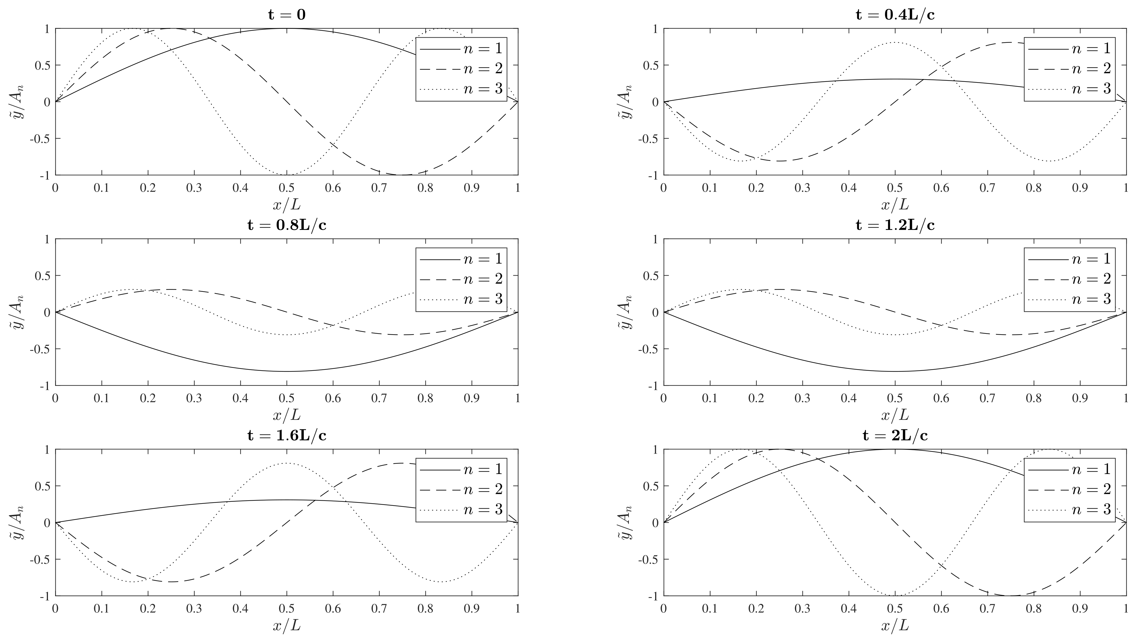
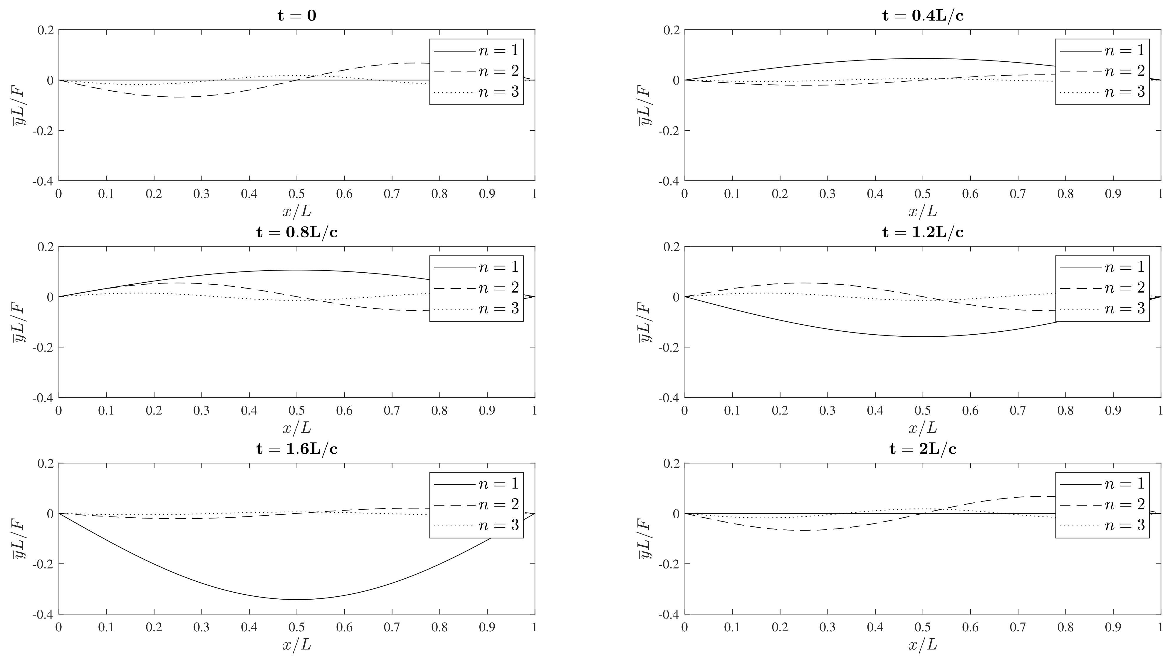
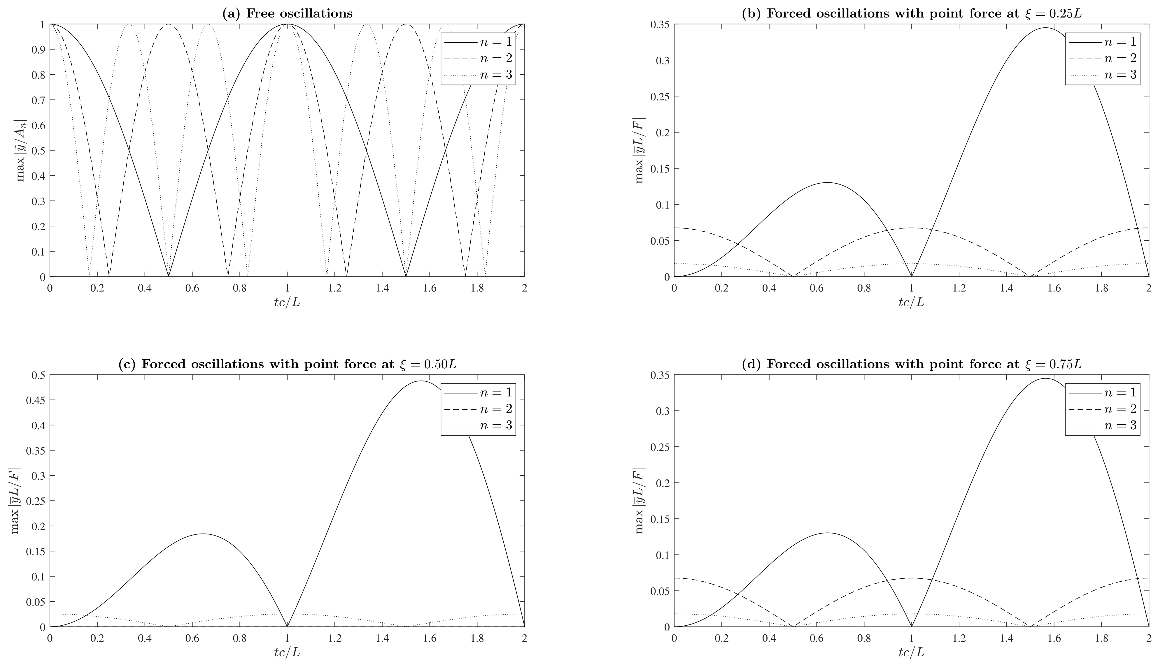
2. Free Oscillations and Forcing by Concentrated Force

Consider the linear free vibrations of an elastic string that are described by the classical wave equation:
2 y ˜ x 2 1 c 2 2 y ˜ t 2 = 0 ,
with wave speed c specified by:
c T ρ ,
where ρ is the mass density per unit length and T is the tangential tension, both assumed to be constant. The string is fixed at the two ends at x = 0 and x = L :
y ˜ 0 , t = 0 = y ˜ L , t .
The transverse displacement is given by a superposition of normal spatial modes,
y n x = sin n π x L ,
with sinusoidal oscillations in time:
y ˜ x , t = n = 1 y n x P n cos n π c t L + Q n sin n π c t L .
The last solution is obtained with the method of separation of variables t and x. The amplitudes are determined by the initial deflection:
y ˜ x , 0 = n = 1 P n sin n π x L ,
and initial velocity:
y ˜ t x , 0 = π c L n = 1 n Q n sin n π x L ,
of the string at time t = 0 . From the sine series (4a) and (4b) follows that the coefficients P n and Q n are specified respectively by the initial displacement:
P n = 2 L 0 L y ˜ x , 0 sin k n x d x ,
and initial velocity:
Q n = 2 π c n 0 L y ˜ t x , 0 sin k n x d x ,
where k n denotes the wavenumber of the mode n:
k n n π L .
The corresponding wavelength is:
λ n 2 π k n = 2 L n .
The wave period is:
τ n λ n c = 2 L n c ,
and the frequency is:
ω n 2 π τ n = n π c L = k n c .
The partial amplitudes P n , Q n may be replaced by the amplitude A n and phase α n :
P n = A n cos α n ,
Q n = A n sin α n ,
with inverses:
A n = P n 2 + Q n 2 1 / 2 ,
tan α n = Q n P n .
In particular, if the string has no deformation at the initial time, y ˜ x , 0 = 0 , then P n = 0 or equivalently α n = π / 2 . In contrast, if the string is released without velocity, y ˜ / t x , 0 = 0 , then Q n = 0 and therefore α n = 0 . Substituting (7a) and (7b) in (3b), the total oscillation is given by
y ˜ x , t = n = 1 A n sin k n x cos ω n t α n .
The phase α n of each mode may be eliminated by changing time to:
t = t α n ω n ,
so that:
cos ω n t α n = cos ω n t .
Thus there is no loss of generality in the following figures to set α n = 0 , since this is equivalent to a time shift.
The Figure 1 shows the dimensionless amplitudes, y ˜ / A n , of the free oscillations for the first three natural frequencies, n = 1 , 2 , 3 . The plots show the oscillations along the string as a function of the dimensionless coordinate, x / L . In the case of Figure 1, the string is released without velocity, therefore Q n = 0 = α n and A n = P n . Otherwise, if the string is released with some velocity, then α n 0 and that case is equivalent to a time shift (9a), implying (9b), of the plots in the Figure 1. According to (8), once the value of time shift α n is defined, the shape of the string is dependent on the dimensionless parameter x / L , and for each natural frequency it is plotted at six different times:
t = 0.0 , 0.4 , 0.8 , 1.2 , 1.6 , 2.0 L / c .
The total deformation of the string is the sum of all the contributions of each natural mode of shape (for each value of n). The deformation is dominated by the natural modes with larger values of A n (in modulus). That influence depends only on the initial deflection, that is, on the shape of the string at the initial time.
The Figure 1 illustrates the shape of the string at six equally spaced times between t = 0 and t = 2 L / c . Each term of y ˜ is proportional to cos ω n t that is a periodic function. Its period is given by (6c). Consequently, the first mode of deformation has period equal to 2 L / c . Considering the second mode, the lowest period is 2 L / 2 c = L / c , implying that the 2 L / c is also a period of the second mode. Generally, each mode of deformation of frequency ω n has the lowest period equal to 2 L / n c (increasing the mode of deformation n, the period decreases) and therefore, multiplying it by n, 2 L / c is also the period of each mode. That is the reason why the Figure 1 illustrates the deformation from the initial time t = 0 until the instant t = 2 L / c because it is the period of each mode of deformation (note that the plots are the same for the two instants). In particular, for n = 2 the string made two complete oscillations, and for n = 3 the string made three complete oscillations, at the final instant t = 2 L / c . The Figure 1 shows that the string is always fixed at the two ends for any mode of deformation all the time. Furthermore, for each mode n, the string has n peaks and n 1 nodes (not counting both ends of the string). These nodes and peaks remain at the same positions all the time due to the separation of variables t and x in the solution. According to the Figure 1, the plots are the same for the instants t = 0.4 L / c and t = 1.6 L / c . The temporal dependence of the oscillation y ˜ is cos ω n t and because cos t 1 = cos 2 L / c t 1 for any instant t 1 , the free oscillation has the property y ˜ x , t = y ˜ x , 2 L / c t . The plots are also the same when t = 0.8 L / c and t = 1.2 L / c for the same reasons. However, the direction of the movement of the oscillation, that is determined by y ˜ / t , is not the same. For example, at the instant t = 0.4 L / c , the string of the first natural mode oscillation ( n = 1 ) is moving downwards while the same string at the instant t = 1.6 L / c is moving upwards.
Consider next the vibrations caused by a force, of frequency ω and amplitude F, concentrated at the point x = ξ :
2 y ¯ x 2 1 c 2 2 y ¯ t 2 = F δ x ξ cos ω t + β ,
where δ is the Dirac delta function [125,126], that can be used to represent a concentrated force. The time dependence of the concentrated force is sinusoidal with applied frequency ω ; this is one term of the representation by a Fourier series of any function of time with bounded fluctuation [127]. In (11) was introduced a phase shift β of the forced oscillation generally distinct from the phase shift α n of the free oscillations (8), that is determined through the Equation (7d) by the initial conditions (5a) and (5b). The response will have the same frequency and the same phase shift as the applied force:
y ¯ x , t = B x cos ω t + β ,
leading to the differential equation:
d 2 B d x 2 + ω c 2 B x = F δ x ξ ,
that can be solved by expanding the Dirac delta function in sine series in the interval 0 , L :
δ x ξ = n = 1 a n sin n π x L .
This assumes that mathematically F is repeated at all ξ + n L positions with n = 1 , 2 , 3 , , and with reversed sign F at ξ m L with m = 0 , 1 , 2 , , so that it specifies an odd function of x, with sine series (13a) with coefficients:
a n = 2 L 0 L δ x ξ sin n π x L d x = 2 L sin n π ξ L .
Substituting (13b) in (13a) follows that the Dirac delta function is represented by the Fourier sine series:
δ x ξ = 2 L n = 1 sin n π ξ L sin n π x L .
Then, substituting the function δ x ξ in (12b), with k ω / c , leads to:
d 2 B d x 2 + k 2 B = 2 F L n = 1 sin k n x sin k n ξ ,
and suggests the solution:
B x = n = 1 b n sin k n x ,
leading to the condition:
k 2 k n 2 b n = 2 F L sin k n ξ .
Substituting (15b) in (15a) and then in (12a), the forced oscillations are given by
y ¯ x , t = 2 F L cos ω t + β n = 1 1 k 2 k n 2 sin k n ξ sin k n x ,
for wavenumber k outside resonance, k k n , and for all n = 1 , , .
In the resonant case, k = k m for some integer m, hence the m-th term of (16) would appear to be infinite. This is physically absurd, because the oscillation cannot have infinite amplitude or energy. It is the result of mathematical error, namely dividing (15b) by zero, k 2 k m 2 = 0 , when k = k m . Thus, the m-th term of (16) is invalid as a solution of (14) if k = k m or ω = ω m . To find a valid solution in this case [122,128], the Equation (15b) is rewritten with the time dependence:
ω 2 ω m 2 b m cos ω m t + β = 2 F c 2 L sin k m ξ cos ω m t + β .
Differentiating with regard to ω m to both sides of (17) leads to:
ω 2 ω m 2 b m t sin ω m t + β 2 ω m b m cos ω m t + β = 2 F c 2 L sin k m ξ t sin ω m t + β ,
and letting ω tending to ω m yields:
b m cos ω m t + β = F c 2 ω m L sin k m ξ t sin ω m t + β .
Using the last equality (19) in the m-th term of (15a) and (15b), while the remaining terms n m are unchanged, leads to the forced response:
y ¯ x , t = F k m 2 L sin k m ξ sin k m x ω m t sin ω m t + β + 2 F L n = 1 n m k m 2 k n 2 1 sin k n ξ sin k n x cos ω m t + β ,
consisting of oscillations of constant amplitude at all wavenumbers k n k m , except k m , for which the amplitude increases linearly with time.
The Figure 2 shows the modified amplitudes, y ¯ L / F (it is not dimensionless), of the forced oscillations for the first three natural frequencies, n = 1 , 2 , 3 . As in the Figure 1, the plots shown the oscillations along the string as a function of the dimensionless coordinate, x / L . According to (20), and bearing in mind (6a), the position x appears always divided by L, in the dimensionless coordinate x / L . The total deformation of the string due to the external force is the sum of all the contributions of each natural mode of shape (for each value of n). The first three contributions are plotted in the Figure 2. In contrast with the free oscillation, the force F contributes equally to each deformation plotted in the Figure 2 for each value of n (and to the contributions not depicted in Figure 2 for n 4 ) because forcing by an impulse in (13a) is equivalent to “white noise”. The total forced deformation is obtained summing each deformation and then multiplying it by F / L . Also, in contrast to the free oscillations, the forced oscillations do not depend on boundary conditions, that is, on the coefficients P n and Q n . In the Figure 2, it is assumed that the point force applied at ξ = 0.25 L . Consequently, the term sin k n ξ that appears in the solution is equal to sin n π / 4 . The forced frequency of the excitation is equal to the first natural mode of free oscillation, that is, the figure is obtained with ω m = ω 1 = π c / 2 L ( m = 1 ). Consequently, at the initial time ( t = 0 ), the string remains horizontal ( y ¯ = 0 ) for the first mode of deformation ( n = 1 ) because, according to (20), the resonant term is proportional to the time. Moreover, the Figure 2 is obtained with β = 0 , which corresponds to a maximum amplitude of the oscillatory applied force at the initial time, according to the right-hand side of (11). The plots would be similar with β 0 , since β only introduces a phase shift to the results. Therefore, the plots of the Figure 2 can be obtained with β 0 , but for times distinct than those indicated above each plot of the figure. The exception is the resonant term because it also depends on the term ω m t .
The Figure 2 shows the string at six times between t = 0 and t = 2 L / c , the same as in the Figure 1. Each term of y ¯ is proportional to cos ω t that is a periodic function. Its period is 2 π / ω and in the particular case of Figure 2 is equal to 2 π / ω 1 = 2 L / c . For that reason, the Figure 2 illustrates the deformation from the initial time t = 0 until the instant t = 2 L / c because it is the period of all modes of deformation (note that the plots are the same for the two instants, although the deformation of the resonant mode, n = 1 , is not periodic because it is proportional to ω m t .). As opposed to the free oscillations, the period of each mode of oscillation is the same and it depends only on the frequency ω of the force. This was already imposed by the solution in (12a). However, in the resonant mode, when the frequency of the force is equal to one of the natural frequencies of the free oscillation, the resonant term is not periodic because the oscillation grows linearly with ω m t .
As in the free oscillations, the Figure 2 shows that the string is always fixed at the two ends for any mode of forced deformation all the time. Furthermore, for each mode n, the string has n peaks and n 1 nodes (not counting both ends of the string). These nodes and peaks remain at the same positions all the time due to the separation of variables t and x in the solution. Moreover, the nodes and peaks of the forced oscillations are at the same position as those of free oscillations. Therefore, all the terms of forced oscillations have the same properties as the free oscillations (the only difference is the period of the oscillations as explained before). The only exception is in the resonant term where the amplitude of oscillation increase with time due to the term ω m t . Another property in common with free oscillations is that the plots of the non-resonant forced oscillations are the same for the instants t = 0.4 L / c and t = 1.6 L / c . The temporal dependence of the oscillation y ¯ is again cos ω t + β and therefore theses oscillations have the property y ¯ x , t = y ¯ x , 2 π / ω t , or in particular case of the Figure 2, y ¯ x , t = y ¯ x , 2 L / c t . However, as in the free oscillations, the direction of the movement of the oscillation, that is determined by y ¯ / t , is not the same. The plots of the non-resonant oscillations are also the same when t = 0.8 L / c and t = 1.2 L / c for the same reasons. This property does not hold with the resonant term due to the term ω m t (in the Figure 2, the resonant oscillation is the plot of n = 1 ). It should also be noted that the resonant and non-resonant oscillations have phases in quadrature, hence when the non-resonant oscillation has maximum amplitude, the resonant oscillation has zero deformation, and vice-versa. This can be changed using the phase shift β in the forced oscillation, for example β = α n + π / 2 would bring the free and forced oscillations in phase.
The total oscillation, that is free plus forced oscillation:
y x , t = y ˜ x , t + y ¯ x , t ,
is given, for ω ω n , by:
y x , t = n = 1 sin k n x A n cos ω n t α n + 2 F L k 2 k n 2 1 sin k n ξ cos ω t + β ,
in the absence of resonance, and, for ω = ω m , by:
y x , t = n = 1 n m sin k n x A n cos ω n t α n + 2 F L k m 2 k n 2 1 sin k n ξ cos ω m t + β + sin k m x A m cos ω m t α m + F k m 2 L sin k m ξ ω m t sin ω m t + β ,
in the presence of resonance. Note that even in the case of zero phase shift, α n = 0 = β , in neither case the forced oscillation can exactly cancel the free oscillation, because: (i) in the non-resonant case (22) the frequencies ω ω n are different; (ii) in the resonant case (23) the frequency is the same ( ω = ω m in the last term), but the amplitudes are different, since it is constant for the free oscillation, but is increasing linearly with time for the forced oscillation.
The plots (a) of the Figure 3 show the maximum amplitude (in modulus) of the free oscillations over time for the first three natural modes of oscillation, n 3 . The other three plots of the Figure 3 show the maximum amplitude (in modulus) of the forced oscillations, each one for a different location of the applied force. In all three plots, the frequency of the force is equal to the first natural mode of the free oscillation, that is, ω = ω 1 = π c / L . Therefore, the plots for n = 1 represent the maximum amplitude of the resonant term. The Figure 3 shows the results for the instants between t = 0 and t = 2 L / c because 2 L / c is the period of all free oscillations. Since 2 L / c is also the period of the applied force, the forced oscillations also have the same period. Note that in these plots, there is no phase shift of the free oscillations and applied force, α n = 0 = β . If α n 0 , there is a phase shift on the result of n mode of oscillation, visualized in the plots (a) of the Figure 3. Setting β 0 introduces a phase shift on all n non-resonant modes of forced oscillations, while on the m resonant mode, the plot is also modified, but not with a phase shift due to the term ω m t .
The maximum amplitude of the free oscillations over time has also an oscillatory behaviour. Indeed, the maximum amplitudes over time can be deduced from (8), knowing the parameters α n and A n , and assuming the maximum value for sin k n x , equal to 1. Consequently, the maximum amplitude of free oscillations, for each mode of vibration n, is proportional to cos ω n t α n . Therefore, the maximum amplitude can reach the value A n when t = L k / n c + L α n / n c π with k being a natural number. The number of times the maximum amplitude of the free oscillations occurs is greater when the value of n is decreased because the period of the oscillations is lower. These conclusions are similar when α n 0 .
The oscillatory behaviour is also present in the forced oscillations over time. The times at which the maximum amplitude occurs depend on the frequency of the applied force, not on its location, as shown in the Figure 3 for β = 0 . In this situation, all the non-resonant terms have maximum amplitude when t = k π / ω (in this case, when t = L k / c ) with k being a natural number. The maximum amplitudes occur when the applied oscillatory force is also maximum. Indeed, this result can be deduced from (22) assuming cos ω t = ± 1 . For the non-resonant oscillations, the maximum amplitude is greater when k n approaches the value k from the applied force (in the case of Figure 3, the greatest amplitudes of non-resonant forced oscillations are for n = 2 because it is the mode of oscillation that is closest to the frequency of the applied force n = 1 ). However, this property is not always true due to the value sin k n ξ . For instance, when the force is applied at the middle of the beam, ξ = 0.5 L , the non-resonant oscillation for n = 2 is null (therefore, the oscillation for n = 3 is greater). This exception results from (23) for the second term ( n = 2 ), knowing that sin k 2 ξ = 0 . The Figure 3 also shows that the maximum amplitudes of the resonant term (in this case for n = 1 ) increases over time because of the term ω m t in (23). Also, the maximum amplitudes of the non-resonant oscillations happen when the resonant oscillation is zero, because when cos ω t = ± 1 , then sin ω t = 0 . The maximum amplitudes of the resonant oscillation occur when sin ω t + ω t cos ω t = 0 . These conclusions are similar when β 0 .
Next is investigated to what extent the forced oscillation can be used to reduce the energy of the free oscillation.

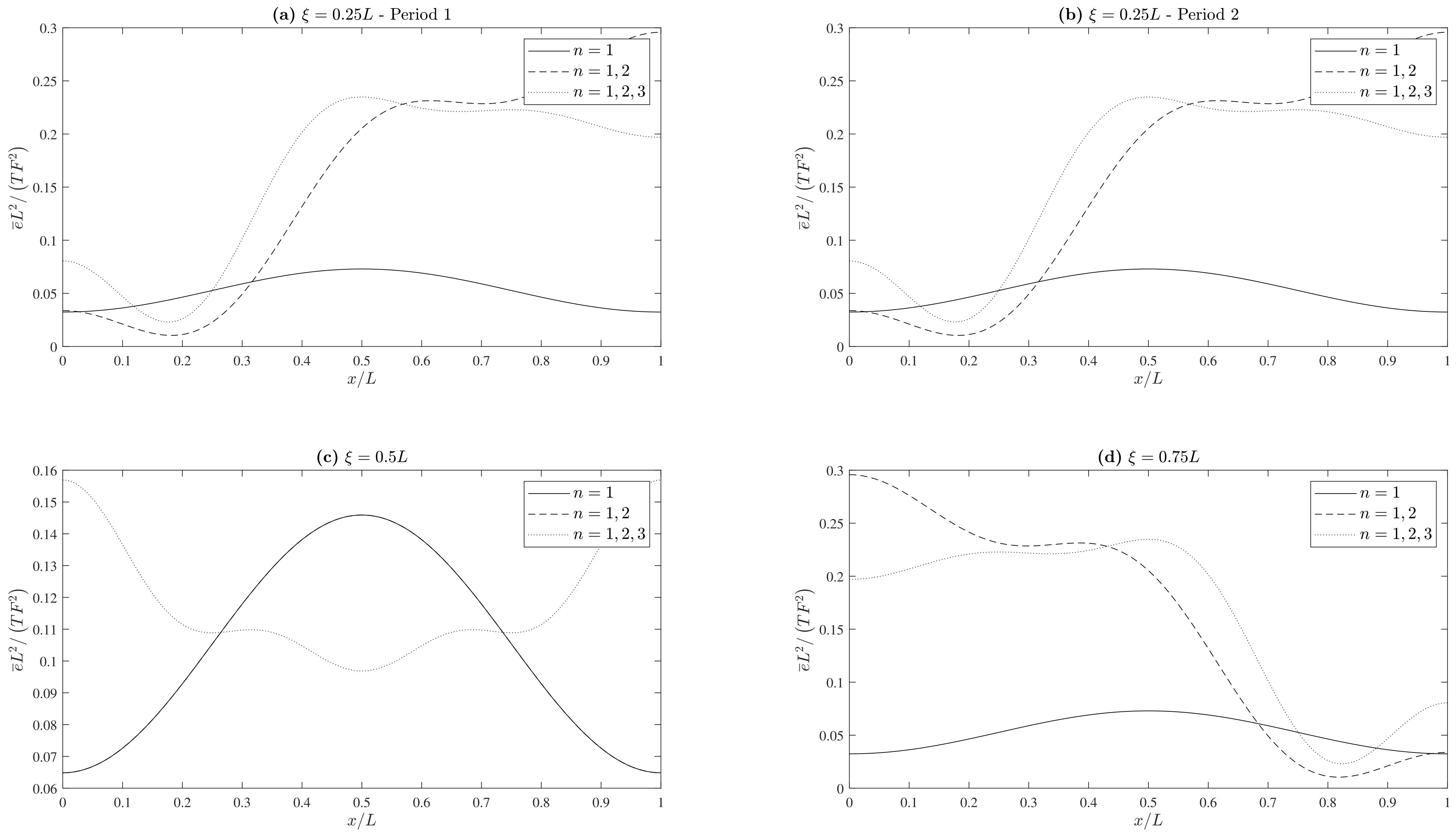
3. Minimization of Total (Kinetic Plus Elastic) Energy

The time average over a period τ is defined by:
f ω t 1 τ 0 τ f ω t d t ,
and can be reduced to an integration along a unit circular arc, assuming the period τ as 2 π / ω , specified by:
0 t < τ = 2 π / ω 0 θ ω t < ω τ = 2 π ,
in the integral:
f θ = 1 2 π 0 2 π f θ d θ
The total energy density per unit length averaged over a period is:
e ˜ x = ρ 2 y ˜ x , t t 2 + T 2 y ˜ x , t x 2 ,
where the kinetic energy involves the mass density per unit length ρ and the elastic energy involves the tangential tension T. For a free oscillation with displacement (8), each mode n of vibration has period equal to τ = 2 π / ω n , as in (6d). The velocity has a mean square over a period given by:
y ˜ x , t t 2 = n = 1 r = 1 A n A r ω n ω r sin k n x sin k r x sin ω n t α n sin ω r t α r ,
and the strain has a mean square over a period given by:
y ˜ x , t x 2 = n = 1 r = 1 = A n A r k n k r cos k n x cos k r x cos ω n t α n cos ω r t α r .
The average over a period of the product of sines and cosines with different phases is given by (A1) and (A2) in the Appendix A:
sin ω n t α n sin ω r t α r = 1 2 δ n r = cos ω n t α n cos ω r t α r
where δ n r is the identity matrix. Thus the average kinetic energy is given by
e ˜ k = ρ 2 y ˜ x , t t 2 = ρ 4 n = 1 ω n A n 2 sin 2 k n x ,
and the average elastic energy is given by
e ˜ e = T 2 y ˜ x , t x 2 = T 4 n = 1 k n A n 2 cos 2 k n x .
Using the wave speed (1a) in ρ ω n 2 = ρ k n c 2 = T k n 2 , the total energy per unit length of string, which is the sum of average kinetic and elastic energies, is constant:
E ˜ 4 e ˜ x T = 4 e ˜ k x + 4 e ˜ e x T = n = 1 A n k n 2 > 0 ,
for the free oscillation.
The Table 1 shows the total energy density of the free oscillations along the string averaged over one period, for the first four modes of the vibration n. In this case, the total energy is constant along the string, not depending on explicit values of position x. The results of the Table 1 are obtained from (29) which follows from the mean square velocity (28a) and the mean square strain (28b). To obtain the mean squares, the values of sin ω n t α n sin ω r t α r and cos ω n t α n cos ω r t α r were needed. The time averages of the product of sines and cosines are calculated over a period in Appendix A; the period of both functions for the time average, sin ω n t α n sin ω r t α r and cos ω n t α n cos ω r t α r , is 2 L / c for any combination of the values n and r (although in some cases the lowest period is L / c or even lower). The phase shifts α n and α r do not change the period of both functions. Therefore, in the Table 1, the first period is from t = 0 until t = 2 L / c , the second period is from t = 2 L / c to t = 4 L / c , and so on.
As indicated by the Equation (29), the energy density is constant along the string for each mode of free oscillation n. The energy density increases with n because A n appears to the square in (29). Also modes with larger A n in modulus, A n , contribute more to the energy. For the same value of A n , modes of higher order n contribute more to the energy because k n increases with n in the respective energy density. Another property is that the contribution of each mode of oscillation n to the energy density is independent of the other modes of oscillation. Therefore, it is possible to show in a tabular form the contribution to the energy for each mode of oscillation separately, as outlined in the Table 1. The energy remains unchanged when the oscillations advance one period, because the time averages have the same values, so the results in the Table 1 are the same for different periods. Hence, the period used to perform the time average is irrelevant in the evaluation of the energy density of free oscillations.
The total energy averaged over a period for the forced oscillation is given by:
e ¯ x = 1 2 ρ y ¯ x , t t 2 + 1 2 T y ¯ x , t x 2 ,
leading by (12a) to:
e ¯ x = 1 4 ρ ω 2 B x 2 + 1 4 T d B d x 2 .
To obtain the last result, one of the intermediate steps is to evaluate the time averages of sin 2 ω t + β and cos 2 ω t + β because, according to (12a), the forced oscillation is proportional to cos ω t + β . The period of both functions is 2 π / ω (although the lowest period is π / ω ), noting that the phase shift of the applied force β does not change the period. Both time averages are equal to 1 / 2 , as shown in Appendix A. Using (15a) in (31), it follows that the energy of forced oscillations is:
E ¯ 4 e ¯ x T = k 2 n = 1 b n sin k n x 2 + n = 1 k n b n cos k n x 2 .
In the non-resonant case, where the frequency of the force ω is not equal to any of the natural frequencies of the free oscillation ω n , the Equation (15b), for which k k n , leads to:
E ¯ = k 2 2 F L n = 1 1 k 2 k n 2 sin k n ξ sin k n x 2 + 2 F L n = 1 k n k 2 k n 2 sin k n ξ cos k n x 2 > 0 ,
showing that the total energy density of the forced oscillation (33) is not constant along the string, unlike for the free oscillation (29), although both are positive. Moreover, the external force supplies energy to all forced n modes of oscillation, in contrast with the free oscillations, where in some n modes the contribution to the energy is zero when A n = 0 .
The Figure 4 shows the energy density of the forced oscillations along the string averaged over some period, for the first tree modes of the vibration n. The results of the Figure 4 are obtained from (33). Contrary to the free oscillations, the energy of forced oscillations for a certain mode n is coupled to the energy of all other modes of oscillation, as deduced from (33). It is not possible to plot the energy for a single mode of oscillation, in contrast to the Table 1 in which the energy values are indicated for each mode separately. Therefore, in the Figure 4: the solid line represents the contribution of the first mode of oscillation, n = 1 ; the dashed line corresponds to the first two modes of oscillation, n = 1 and n = 2 combined, as if the two series in (33) was truncated after the second term; the dotted line is obtained with the same two series truncated after the third term, n = 1 to n = 3 . As explained before, the period τ in which the time averages were performed is 2 π / ω . Hence, in the Figure 4, specifically in the plots (a) and (b), the period 1 is from t = 0 until t = 2 π / ω and the period 2 is from t = 2 π / ω until t = 4 π / ω .
As indicated by the Equation (33), the energy density is not constant along the string and exhibits an almost oscillatory behaviour. The plots also show that using only the first three terms in the series of (33) is not accurate to represent the energy density and therefore more terms of the series should be used, although some properties can be verified. The contribution of each mode of oscillation n to the forced energy density is coupled to all the other modes of oscillation. Similar to the free oscillations, the energy remains unchanged when the forced oscillations advance one period, hence the plots (a) and (b) of the Figure 4 are the same for different periods. Consequently, the period used to perform the time average is also irrelevant in the evaluation of the energy density of forced oscillations (that is the reason why, in the plots (c) and (d), the period number is not stated because they are equal whatever the period). This property holds for any location ξ and frequency ω of the applied force.
Concerning the total energy of the total or combined (free plus forced) oscillation:
e x = 1 2 ρ y x , t t 2 + 1 2 T y x , t x 2 ,
since in the outside resonance the frequencies are different with ω ω n , the cross-products of sines and cosines have zero average over a period if the ratio of ω to some natural frequency ω n is equal to a rational number, recalling (A3) to (A5) in the Appendix A:
cos ω n t α n cos ω t + β = 0 = sin ω n t α n sin ω t + β ,
and the energy is the sum of the parts due to the free and forced oscillations:
e x = e ˜ x + e ¯ x
with:
E = 4 e x T = E ˜ + E ¯ > E ˜ .
If the frequency of the force ω is not equal to some rational number times the natural frequency ω n , the functions cos ω n t α n cos ω t + β and sin ω n t α n sin ω t + β may not be periodic and consequently their time averages to evaluate the integral in (24a) may result in a non-zero value. In that case, an additional term appear on the right-hand side of (36a) that represents the coupling between free and forced oscillations. Anyway, if starting with a free vibration consisting of normal modes, forcing at any other frequency will only serve to increase the energy. Thus, if the energy of the free oscillation can be reduced at all, it must be through forcing at a natural frequency, which then leads to resonance. It is investigated next whether it is feasible or not to prevent energy growth at an undamped resonance condition, and for how long.
Concerning forcing at a natural frequency with ω = ω m , for all terms n m , the functions cos ω n t α n cos ω m t α m and sin ω n t α n sin ω m t α m are always periodic (Appendix A) with τ = 2 L / c (it may not be the lowest period). Therefore, the result (35) holds when ω = ω m for certain m. Consequently, forcing at a natural frequency, for all terms n m , leads to the same result (22) as before, that is, the energies of the free and forced oscillations add up to (36b). Hence can be singled out for further analysis only the resonant term, specifically the second term on the right-hand side of (23), that is:
y m x , t = sin k m x A m cos ω m t α m + F k m 2 L sin k m ξ ω m t sin ω m t + β ,
and the subscript m can be omitted in the sequel, corresponding to the change of notation k m , ω m , A m , α m k , ω , A , α , which cannot cause any confusion henceforth.
The total energy (kinetic plus elastic) of the total (free plus forced) resonant oscillation, for the resonant mode n = m , written explicitly in (37), is:
2 e m ρ = y m x , t t 2 + c 2 y m x , t x 2 .
It involves two terms: the first term, evaluated for the first period, is:
y m x , t x 2 = k 2 cos 2 k x A 2 cos 2 ω t α F k 2 L 2 + F k 2 L 2 sin 2 k ξ ω t 2 sin 2 ω t + β + 2 A F k 2 L sin k ξ ω t cos ω t α sin ω t + β F k 2 L 2
and the second term, also evaluated for the first period, is:
y m x , t t 2 = ω 2 sin 2 k x A 2 sin 2 ω t α F k 2 L 2 + F k 2 L 2 sin 2 k ξ sin ω t + β + ω t cos ω t + β 2 2 A F k 2 L sin k ξ sin ω t α sin ω t + β + ω t cos ω t + β F k 2 L 2 .
In the last two equations appear the following averages over a period 2 π / ω = 2 L / m c evaluated in Appendix A as (A6) to (A14). The first result,
cos 2 ω t α = 1 2 = sin 2 ω t α ,
is independent of the period (for instance, if the integral in (24a) is evaluated from t = 2 L / m c to t = 4 L / m c , the last result would be equal). Since the last result is independent of the period, the last time average can be evaluated from t = 0 to t = 2 π / ω because τ = 2 π / ω is always a period of the function, regardless the value of α . In the calculation of the energy of forced resonant oscillations, the following averages over a period are also needed:
ω t cos ω t α sin ω t + β = π 2 sin α + β 1 4 cos β α ,
ω t 2 sin 2 ω t + β = 2 π 2 3 π 2 sin 2 β 1 4 cos 2 β ,
sin ω t + β + ω t cos ω t + β 2 = 1 2 + 2 π 2 3 + π 2 sin 2 β 1 4 cos 2 β ,
sin ω t α sin ω t + β + ω t cos ω t + β = cos α + β 2 cos β α 4 π 2 sin α + β .
These last results are only valid for the first “period”, that is, when the integral (24a) is evaluated from t = 0 to t = 2 π / ω . Indeed, none of the last functions to do the time average are periodic functions, due to the term ω t . However, the results are deduced assuming τ = 2 π / ω . Substitution of (40a) to (40e) in the total resonant energy Equation (38) shows that the total energy, averaged over the first period, depends on phase values and on position, in the resonant case:
2 e m x ρ ω 2 = A 2 2 + F k 2 L 2 sin 2 k ξ 2 π 2 3 + 1 2 sin 2 k x A F 2 k 2 L sin k ξ cos β α cos 2 k x + 2 cos α + β sin 2 k x 2 π sin α + β F 2 k 2 L 2 sin 2 k ξ cos 2 β + 2 π sin 2 β cos 2 k x .
The phase α of the free oscillation can be set to zero by suitable choice of initial time. The total energy of the free plus forced resonant oscillation has four terms on the right-hand side of (41): (i) the first is the energy of the free oscillation; (ii) in the second term adds to the total energy, and is independent of the phases α and β ; (iii) the third term, when α = 0 , the factor in square brackets is simplified to cos β 2 π sin β , and hence this term does not have a fixed sign, but reduces the total energy most for the forcing phase shift β = 2 arctan 2 π / 1 + 1 + 4 π 2 , when the factor in square brackets is 1 + 4 π 2 ; (iv) the fourth term does not depend on the phase of free oscillations, does not have a fixed sign and the reduction of the total energy due to that term depends not only on the phase β , but also on the value k x . Choosing the phases α = 0 and β = 0 , the total energy is simplified to:
2 e m x ρ ω 2 = A 2 2 + 2 π 2 3 F 2 k 2 L 2 sin 2 k ξ 8 π 2 3 cos 2 k x A F 2 k 2 L sin k ξ .
The Figure 5 shows the energy density of the total resonant oscillation (37) along the string averaged over one period, for the resonant mode of oscillation n = m . For the first period, the plots (a) of the Figure 5 are obtained from (42). The only difference to the other periods are the results of the time averages in (40b) to (40e). Independently of the period, the energy of the resonant oscillation e m has always three terms (as in (42) for the first period). One term is proportional to A 2 and represents the free oscillation for the resonant mode of oscillation n = m . It is represented by the solid lines in the Figure 5. As usual with free oscillations, it is constant along the string and does not change with the period. A second term is proportional to F 2 / L 2 and is due to the forced oscillation in the resonant mode. It corresponds to the dashed lines. As usual with forced oscillations, it is not constant along the string and has an oscillatory term, not dominant because cos 2 k x 1 8 π 2 / 3 26.32 in (42). It also changes with the period because of the time averages (40b) to (40e) that appear in this contribution. The last term is proportional to A F / L and corresponds to the dotted lines. This term represents the coupling between free and forced oscillations in the resonant energy. It is constant along the string and does not change with the period when α = 0 = β as in the Figure 5. It is the only negative term in the energy e m . Otherwise, all the terms are proportional to k 2 and therefore are dependent on the square of the frequency of the force ω 2 . Therefore, for different frequencies of the force, the numeric values would be different, but the shape of the plots (constant for the solid and dotted lines; oscillatory for the dashed line) are unchanged.
Bearing in mind that (42) is the resonant energy density, or energy per unit length, for α = 0 = β , the total resonant energy for the string of length L:
G F , ξ = 2 ρ ω 2 L 0 L e m x d x ,
is given by:
G = 1 2 A 2 + 2 π 2 3 F k 2 L 2 sin 2 k ξ A F 2 k 2 L sin k ξ .
The term “total” energy has been used with three distinct meanings: (i) kinetic plus elastic energies; (ii) energy of the total or combined oscillation, that is free plus forced oscillation; (iii) energy of the string, that is energy density integrated over its length. The function (44), to be optimized, is the “total” energy in all of these three senses, that is the kinetic plus elastic energy density, averaged over one period, for the free plus forced resonant oscillation, integrated along the length of the string. This total energy should be minimized, by optimizing the magnitude F and location ξ of the force; the aim is to check whether, due to the presence of resonant forcing, the total resonant energy over the first period (44), can be made smaller than the energy A 2 / 2 of the free oscillation in the first term.

4. Optimization of Strength and Location of Forcing Effect

Consider first the dependence of the total energy (44), with respect to the magnitude F of the applied force. The latter F = F + is chosen so as to minimize the energy:
G F + = 0 , 2 G F + 2 > 0 .
From (44) it follows that the energy does have a minimum with respect to the magnitude of the force:
2 G F 2 = 4 π 2 3 k 4 L 2 sin 2 k ξ > 0 ;
equating to zero:
G F = sin k ξ 4 π 2 F 3 k 4 L 2 sin k ξ A 2 k 2 L ,
specifies the magnitude of the optimal force:
F + = 3 8 π 2 k 2 L A csc k ξ ,
which minimizes the total energy:
G + G F + , ξ = 1 2 A 2 1 3 16 π 2 .
This optimal result does not depend on the point of application of the force. Compared with the energy of the free oscillation:
G 0 = 1 2 A 2 ,
optimal forcing at resonance provides a very small reduction of energy:
G + G 0 = 1 3 16 π 2 = 0.981 ,
of less than 2%, over the first period. Since resonant forcing causes an oscillation of amplitude increasing with time, it is clear that even with optimal forcing, the total energy will exceed that of the free vibration, for a time span slightly longer than a period. Thus, active suppression of a normal mode by a resonant point force can be achieved very marginally, for a time span of at most one period.
It is shown next that the total energy has a maximum with respect to the point of application ξ of the concentrated force:
G ξ ± = 0 , 2 G ξ ± 2 < 0 .
Substituting (44) in the first condition of optimization (51) leads to:
0 = G ξ = F k L cos k ξ A 2 + 4 π 2 3 F k 2 L sin k ξ .
There are two sets of stationary values: one coincident with (48):
sin k ξ + = 3 8 π 2 A k 2 L F + ,
and one different:
cos k ξ = 0 .
Since the minimization with regard to F did not depend on ξ in (49), it may be expected that the second set (53b) is not a minimum. Indeed, from (44) or (52), it follows that:
2 G ξ 2 = A F 2 L sin k ξ + 4 π 2 3 F k L 2 1 2 sin 2 k ξ .
In particular for the second set of roots (53b), it implies sin k ξ = ± 1 , and the second condition of optimization (51) leads to:
2 G ξ 2 ξ = ξ = F 2 L ± A 8 π 2 3 F k 2 L < 0 ;
the last expression is negative for − sign and also for + sign with F > 3 / 8 π 2 k 2 L A in (48), so the second condition of (51) is met. For the first set of roots (53a):
2 G ξ 2 ξ = ξ + = 1 3 2 π F k L 2 3 k A 4 π 2 = 4 π 2 3 k 2 L 2 F 2 3 k 2 L A 8 π 2 2 < 0 ,
so the second condition of (51) is met again. Thus, the case F = F + is a minimum at constant ξ , but ξ = ξ ± is a maximum at constant F. The maximum ξ = ξ at constant F in (53b) would correspond in (48) to:
F = 3 k 2 L A 8 π 2 csc k ξ = ± 3 k 2 L A 8 π 2 .
The minimum for F in (48) with ξ fixed, and the maximum for ξ in (53a) and (53b) with F fixed, are particular cases of the general case when both F and ξ can vary.
The most general approach is to regard the total energy (44) as a joint function of magnitude F and location ξ of the applied force, so that the conditions of stationarity are:
G F = 0 , G ξ = 0 ,
and the second-order differential is:
d 2 G = 2 G F 2 d F 2 + 2 G ξ 2 d ξ 2 + 2 2 G F ξ d F d ξ .
The second-order differential specifies (i) a global minimum if it is positive, (ii) a maximum if it is negative, and (iii) an inflexion or higher-order extremum if it is zero. Since G is (a) maximum (51) with regard to ξ at fixed F and (b) minimum (45) with regard to F at fixed ξ , this suggests the case (iii) of inflexion or higher-order extremum, with the condition
Δ 2 G / F 2 2 G / F ξ 2 G / F ξ 2 G / ξ 2 = 0 .
The condition (59) involves a cross-derivate which can be evaluated from (47) leading to:
2 G F ξ = cos k ξ 8 π 2 F 3 k 3 L 2 sin k ξ A 2 k L .
The second order derivatives of (44) in (46), (54) and (60) are given, for the case (48)≡(53a), which includes (56) by:
2 G F 2 ξ = ξ + = 3 A 4 π F 2 ,
2 G ξ 2 ξ = ξ + = 1 3 2 π F k L 2 3 k A 4 π 2 ,
2 G F ξ ξ = ξ + = ± A 2 k L 1 3 k 2 L A 8 π 2 F 2 1 / 2 .
It can be checked that the determinant is zero,
Δ = 2 G F 2 2 G ξ 2 2 G F ξ 2 = 0 ,
confirming (59).
The Figure 6 provides an overview of the total resonant energy, given by (44), in the plane of the parameters F / L and ξ / L , the last one between 0 and 1. The values of the contour lines result from the difference between the resonant energy and the free oscillation energy, that is, G A 2 / 2 , for the first period. It means that the value 0 of the contour plot happens when the forced resonant energy is zero, in other words, when the total resonant energy equals only the free oscillation energy, G = A 2 / 2 . The values of the contour plots depend also on the explicit value of A, because of the third term of (44). In this case, the Figure 6 is obtained setting A = 1 . Each plot corresponds to a different resonant frequency. For example, the plots (a) of the Figure 6 corresponds to the frequency of the applied force ω equal to the first natural frequency of the free oscillation, ω 1 . The thick red line highlights the combination of the values of the parameters F / L and ξ / L for a minimum possible resonant energy G.
Although the resonant energy depends on the two parameters F and ξ simultaneously, according to (44), the parameters are combined only in the form F sin k ξ . The resonant energy can be interpreted as a quadratic equation of the combined parameter F sin k ξ , that is, G = c 1 F sin k ξ 2 + c 2 F sin k ξ + c 3 with c 1 > 0 . Consequently, the minimum of the value of the resonant energy G is given by F sin k ξ = c 2 / 2 c 1 which corresponds to the Equation (48) and to the thick red lines presented in the Figure 6. The figure shows therefore that the minimum value of the resonant energy can be obtained with a force applied at any position of the string, except at the points where sin k x = 0 . In those positions, regardless the value of the applied force F, the resonant energy equals the free oscillation energy, G = A 2 / 2 , the same effect as if there is no applied force, F = 0 . The contour values, as mentioned before, depend on the value of A; the minimum value of G, according to (49), also depends on the value of A. Furthermore, due to the thick red lines of the Figure 6, there are infinite combinations of the values of both parameters to get the minimum possible resonant energy. Observing the red lines, to reduce the resonant energy, the point force must be applied at a position where cos k x = 0 if it is intended that the force has the lowest possible value. For instance, when ω = ω 1 , the best position to apply a force is at the middle of the string. The worst locations to apply a force are in the vicinity of the positions where sin k x = 0 that are the ends of the string. The number of these best or worst locations to apply a force increases with the resonant frequency.

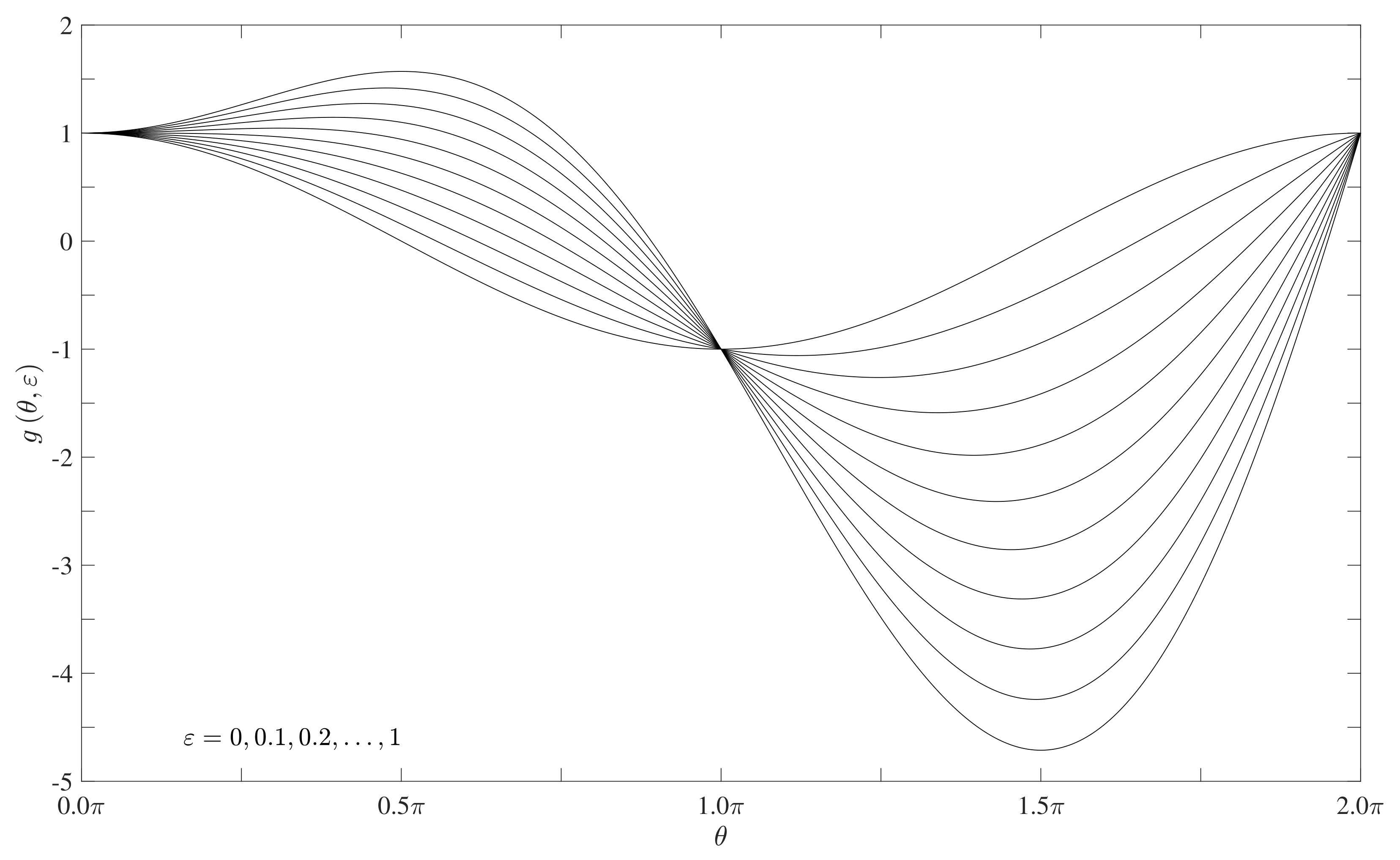
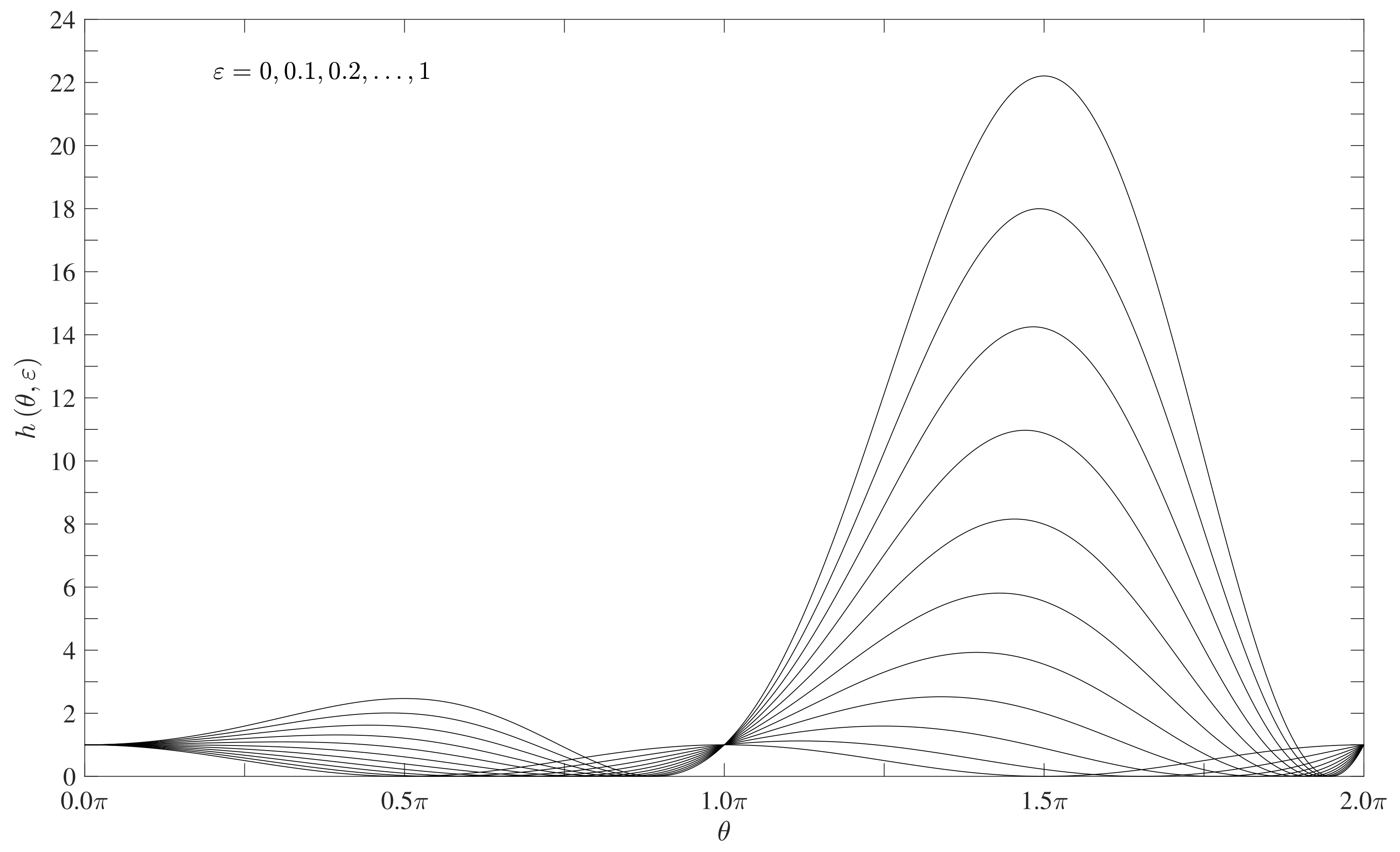
5. Oscillation and Energy for Optimal and Non-Optimal Forcing

The free vibrations of an elastic string consist of a superposition of normal modes. The question addressed in the present paper is whether forcing can be used to suppress totally normal modes, or failing that, at least reduce the energy of the total free plus forced oscillation relative to the energy of the free oscillation alone. Clearly, forcing at a frequency distinct from all natural frequencies will not do: it does not couple to the free motion, and just increases the total energy. Forcing at a natural frequency will cause resonance, that is an amplitude increasing linearly with time, for the forced vibration:
y ¯ x , t = F k 2 L sin k ξ sin k x ω t sin ω t ,
compared to the free vibration:
y ˜ x , t = A sin k x cos ω t .
The total energy over the first period can be marginally reduced (48) if:
F = ε 0 A k 2 L csc k ξ ,
with:
ε 0 3 8 π 2 = 0.038 ,
but for longer time spans it will be increased by any choice of the magnitude of the forcing. The preceding result holds optimizing the magnitude F of the forcing at a fixed location.
The total or combined oscillation is given by:
y x , t y ˜ x , t + y ¯ x , t = sin k x A cos ω t + F k 2 L sin k ξ ω t sin ω t ,
which can be written in the form:
y x , t = A sin k x g θ , ε
with the independent variable θ defined by θ ω t in (24b) and the other independent variable ε as:
ε F / A k 2 L sin k ξ ,
leading to:
g θ , ε cos θ + ε θ sin θ ,
where all the time dependence appears in (66c). The Equation (67) gives an indication of the energy:
h θ , ε g θ , ε 2 .
The functions g and h are plotted respectively in Figure 7 and Figure 8 for small values of ε around ε 0 in (64b):
ε = 0.00 , 0.01 , 0.02 , 0.03 , ε 0 , 0.04 , 0.05 , 0.06 , 0.07 , 0.08 , 0.09 , 0.10 ;
the thick line corresponds to ε 0 and leads to the oscillation (in Figure 7) with the smallest energy or area below the curve in Figure 8. For larger values of ε :
ε = 0.0 , 0.1 , 0.2 , 0.3 , 0.4 , 0.5 , 0.6 , 0.7 , 0.8 , 0.9 , 1.0 ,
the resonance dominates the total oscillation even in the first period, leading to large amplitude (in Figure 9) and energy (in Figure 10).
The conclusion that the energy of the combined oscillation cannot be kept below the energy of the free oscillation, for much longer than a period, applies to a single concentrated force. Use of several concentrated forces or a distributed force would be possible also, and is investigated next.

6. Forcing by Multiple Concentrated Forces

In the case of M forces F m concentrated at the points x = ξ m with m = 1 , , M , the undamped resonant response (63a) would be replaced by:
y ¯ x , t = 1 k 2 L sin k x ω t sin ω t m = 1 M F m sin k ξ m .
This is equivalent by (63a) to a single force F concentrated at ξ , such that:
F sin k ξ = m = 1 M F m sin k ξ m .
Thus, the conclusions are the same, for instance, regarding (64a), the energy over the first wave period can be marginally reduced if:
m = 1 M F m sin k ξ m = ε 0 A k 2 L ,
where A is the amplitude of the free oscillation (63b) and ε 0 is the constant (64b). The difference between (72) and (64a) is that there is a greater choice of pairs F m , ξ m . A further case deserves investigation, namely that of continuously distributed forces.

7. Optimization of Continuously Distributed Forces

In the case of an applied force, which is harmonic in time, with frequency ω and continuously distributed in space, the forced wave Equation (11) is replaced by:
2 y ¯ x 2 1 c 2 2 y ¯ t 2 = f x cos ω t ,
which has a solution (12a), where B x satisfies:
d 2 B d x 2 + k 2 B = f x .
If the spatial force distribution f x is a function of bounded fluctuation in 0 x L , it has [129] a Fourier series representation:
f x = f 0 + n = 1 f n cos k n x + f n sin k n x .
A solution of (74) may be sought as a series:
B x = n = B n x ,
in which the terms satisfy:
d 2 B 0 d x 2 + k 2 B 0 = f 0 ,
d 2 B n d x 2 + k 2 B n = f n cos k n x ,
d 2 B n d x 2 + k 2 B n = f n sin k n x ,
with given f n , k and k n .
In the non-resonant case k k n , the solution of (77a) to (77c) is a sinusoidal oscillation with constant amplitude, for all terms in (78b) and (78c) with n 0 :
B 0 = f 0 / k 2 ,
B n x = f n k 2 k n 2 cos k n x ,
B n x = f n k 2 k n 2 sin k n x ,
except for the term n = 0 in (78a) that is constant. In the case of resonance, k = k m for some m, the solution may be obtained as in (17) to (20), that is differentiating the numerator and denominator with regard to k n , leading to:
B m x = f m 2 k m x sin k m x ,
B m x = f m 2 k m x cos k m x .
The first boundary condition of (2) is not satisfied by (78b), and the second boundary condition is not satisfied by (79b) in general, implying:
f m = f 0 = f 1 = = f m 1 = f m + 1 = f m + 2 = = 0 ,
as restrictions on the applied force (75), that simplifies to:
f x = f m cos k m x + n = 1 n m f n sin k n x .
The forced response of the string is:
B x = f m 2 k m x sin k m x + n = 1 n m f n k 2 k n 2 sin k n x .
Taking a free oscillation of the form (63b), it cannot be suppressed for the same reasons as before: (i) if n m , the last terms on the right-hand side of (82) have a different wavenumber; (ii) if the wavenumber coincides, k = k m , the first term on the right-hand side of (82) shows that the undamped resonance has a growing amplitude which cannot be matched to the remaining term of (82), that is the total, free (63b) plus forced (first term on the right-hand side of (82)) oscillation is:
y * x , t = A + f 2 k x sin k x cos ω t ,
where the index m is again suppressed for brevity, f m , k m , ω m f , k , ω .
As in (36a) and (38), the energy of the total oscillation per unit length of string is given by:
2 E * x ρ y * t 2 + c 2 y * x 2
where the time averages (24a) are evaluated readily, by (A6) and (A7), after substituting (83) into (84), leading to:
2 E * x ρ = ω 2 2 A + f 2 k x 2 sin 2 k x + k 2 c 2 2 A + f 2 k x cos k x + f 2 k 2 sin k x 2 ,
which can be simplified to:
2 E * x ρ = ω 2 2 A + f 2 k x 2 + f 2 k 2 2 sin 2 k x + f 2 k 2 A + f 2 k x sin 2 k x .
The total energy over the length of the string is defined as in (43), namely:
G * f 2 ρ ω 2 L 0 L E * x d x ,
and substitution of (86) in (87) leads to two integrals: (i) the first integral uses k L = 2 π :
f 2 8 k 4 L 0 L sin 2 k x d x = f 2 16 k 4 ;
(ii) the second integral uses β = k x :
1 2 L 0 L f 2 k x f 2 k 2 sin 2 k x d x = f 2 8 k 5 L 0 2 π β sin 2 β d β = π f 2 8 k 5 L = f 2 16 k 4 .
Since (88a) and (88b) add to zero, the total energy over the length of the string (87) follows
G * f = A 2 2 + A f L 4 k + f 2 L 2 24 k 2 .
The total energy has a minimum, since the second order derivative of G * is positive. That minimum corresponds to d G * / d f = 0 leading to the applied force
f * = 3 k A L ,
or in dimensionless form,
f * L 2 A = 3 k L = 6 π .
The minimum energy is:
G * f * = A 2 8 = 1 4 G 0 ,
25% of the energy of oscillation, that is a 75% reduction. Thus, choosing the continuously distributed force (90a) leads, by (82), to a resonant oscillation:
y ¯ x , t = f * 2 k x sin k x cos ω t = 3 2 A x L sin k x cos ω t ;
the latter adds to the free oscillation, to produce a combined oscillation,
y x , t = A 1 3 2 x L sin k x cos ω t ,
which reduces the energy by a factor 0.25 in (91), which is the lowest (because the second derivative is negative) attainable value. This value is lower than the obtainable (50b) with single (48) or multiple (72), (64b) point forces.

8. Conclusions

The question addressed in the present paper is whether the linear undamped free vibrations of an elastic string can be suppressed, or at least their total energy reduced, by using external applied forces concentrated or distributed along its length. The linear undamped free vibrations of an elastic string consist of the superposition of a fundamental mode and harmonics, and two cases are considered, namely the applied frequency of the external forces: (case I) does not coincide with any natural frequency, for non-resonant forcing; (case II) coincides with one of the natural frequencies for resonant forcing. The two cases are quite distinct because: (I) non-resonant forcing has constant amplitude and energy; (II) resonant forcing has amplitude increasing linearly with time, and hence energy increasing quadratically with time, until non-linear effects come into play.
Starting with (I) non-resonant forcing at an applied frequency distinct from all natural frequencies: (i) the energy, that is the sum of kinetic and elastic energies, in constant both for the (a) linear undamped free oscillation and for the (b) linear forced non-resonant oscillation; (ii) the applied frequency being distinct from all natural frequencies, there is no interaction with the free oscillations, whose energy remains the same; (iii) the forced non-resonant oscillation adds a constant energy, so the total energy of free plus forced oscillation is larger than the energy of the free oscillation alone; (iv) this is the reverse of the result sought, and thus non-resonant forcing cannot decrease and instead increases the total energy when superimposed on free oscillations. Thus, if it is possible at all to reduce the energy of free oscillations, it can only be through (II) resonant forcing using either (IIa) concentrated or (IIb) distributed forces, that can be optimized to minimize the total energy.
The reduction of the total energy of oscillation by resonant forcing is possible with two limitations: (i) it applies only to the free oscillation whose natural frequency coincides with the applied frequency, and has no effect on all the other modes; (ii) since the energy of the resonant forced oscillation increases quadratically with time, it will ultimately dominate the total energy over a sufficiently long time, so that total energy reduction is possible only over a short initial time, say the first period of oscillation. Thus, the question being addressed can be rephrased: can the resonant forcing reduce the total energy over the first period of oscillation? Although the answer is “yes” in both cases, the result is quite different for (IIa) concentrated and (IIb) distributed applied forces, using optimization in each case.
In the case (IIa) of single or multiple point forces, the total energy over the first period of oscillation, relative to the free oscillation, can be reduced by a maximum of no more than 2% by resonant forcing at an applied frequency equal to the natural frequency. The less than 2% reduction is a minimum of the total energy obtained by optimizing the magnitude of the applied concentrated force at a fixed location. Since the energy of the forced resonant oscillation increases quadratically with time, this small reduction is quickly overwhelmed beyond the first period of oscillation. The case (IIb) is rather more favourable, since by optimizing the magnitude and spatial variation of the continuously distributed force applied along the length of the string, the resonant forcing reduces the total energy over the first period of oscillation by 75% relative to the free oscillation alone. Since the energy of the forced oscillation increases quadratically with time, it becomes dominant for times moderately beyond one period. These results exclude the effects of damping, that is present in many practical situations, and is considered in the follow-on paper (part II).

Author Contributions

Conceptualization, L.M.B.C.C.; Methodology, L.M.B.C.C. and M.J.S.S.; Software, M.J.S.S.; Formal analysis, L.M.B.C.C. and M.J.S.S.; Investigation, L.M.B.C.C. and M.J.S.S.; Resources, L.M.B.C.C.; Writing—original draft, L.M.B.C.C.; Writing—review and editing, L.M.B.C.C. and M.J.S.S.; Visualization, M.J.S.S. All authors have read and agreed to the published version of the manuscript.

Funding

This work was supported by the Fundação para a Ciência e Tecnologia (FCT), Portugal, through Institute of Mechanical Engineering (IDMEC), under the Associated Laboratory for Energy, Transports and Aeronautics (LAETA), whose grant numbers are SFRH/BD/143828/2019 to M. J. S. Silva and UIDB/50022/2020.

Institutional Review Board Statement

Not applicable.

Informed Consent Statement

Not applicable.

Data Availability Statement

Not applicable.

Conflicts of Interest

The authors declare no conflict of interest.

Appendix A. Averages over a Period

Several averages over a period (24a) to (24b) were used in the text. In all cases, the period τ of the function to be integrated must be determined.
(i) To evaluate the relation (27), the period of the function sin ω n t α n sin ω r t α r has to be determined. The period of the trigonometric function sin ω n t α n is 2 π / ω n = 2 L / n c while the period of sin ω r t α r is 2 L / r c . Generally, the product of the two functions does not result in a periodic function. In this case, 2 L / c is a period of both functions and therefore 2 L / c is also a period of the multiplication of both (however, this does not imply that 2 L / c is the lowest period; in some cases, the lowest period is L / c ). For that reason, the value of τ in (24a) is 2 L / c for any combination of the values of n and r. The integrals in (27) are then given by:
sin ω n t α n sin ω r t α r = 1 2 cos ω n ω r t + α r α n + 1 2 cos ω n + ω r t α r α n = 1 2 δ n r ,
cos ω n t α n cos ω r t α r = 1 2 cos ω n + ω r t α n α r + 1 2 cos ω n ω r t + α r α n = 1 2 δ n r .
where δ n r is the identity matrix. This result follows from the fact that when ω n ω r , the time average is zero, otherwise it is cos α r α n / 2 . But in this last case, when ω r = ω n , meaning the same mode of oscillation, then α r = α n , and so the result is simplified to 1 / 2 .
(ii) In (35), the time averages are:
cos ω t + β cos ω n t α n = 1 2 cos ω + ω n t + β α n + 1 2 cos ω ω n t β α n = 0 ,
sin ω t + β sin ω n t α n = 1 2 cos ω ω n t + β + α n 1 2 cos ω + ω n t + β α n = 0 ,
assuming that ω / ω n = p / q is a rational number so that cos ω ω n t is a periodic function with period:
τ = 2 π ω ω n = 2 π ω n 1 p / q ± 1 = τ n q p ± q .
Generally, let τ 1 be a period of f t and let τ 2 be a period of g t . Suppose that there are two positive integers c 1 and c 2 such that c 1 τ 1 = c 2 τ 2 = τ . Then, the product of the two functions is also a periodic function. The period is τ . On the other hand, if it is not possible to get the positive integers c 1 and c 2 , maybe the function f t g t is not periodic. For example, if f t is sin ω n t α n and has τ 1 = 2 π / ω n = n π c / L as a period, and g t is sin ω t + β and has τ 2 = 2 π / ω as a period, then f t g t is a periodic function if c 1 2 π / ω = c 2 2 π / ω n (meaning that ω / ω n must be equal to a rational number) or equivalently if ω = n c 2 / c 1 π c / L . In this case, if the period of ω n is 2 L / n c , then 2 L / c is also a period of the same function, regardless of the value of n. Consequently, sin ω t sin ω n t is a periodic function if ω = c 2 / c 1 π c / L or if ω L / π c = c 2 / c 1 . The period of the product of both functions is τ = c 1 τ 1 = c 1 π c / L = c 2 τ 2 = c 2 2 π / ω .
(iii) The time averages evaluated in (i) can be simplified when ω n = ω r ω and α n = α r α , leading to the time averages (40a) given by:
sin 2 ω t α = 1 2 ,
cos 2 ω t α = 1 2 ,
where (A6) and (A7) follow from (A1) and (A2) respectively with n = r ;
(iv) The function in (40b) is not periodic due to the term ω t . In this case, it is assumed that τ = 2 π / ω . With this assumption, this last result depends on which “period” the integration is evaluated. For instance, if the limits of the integral are 2 π and 4 π , the result of the integration would not be the same. Using a trigonometric identity and the integration by parts, the time average for the first “period” is equal to:
ω t cos ω t α sin ω t + β = 1 2 π 0 2 π θ cos θ α sin θ + β d θ = 1 4 π 0 2 π θ sin α + β sin α β 2 θ d θ = π 2 sin α + β 1 4 cos β α .
(v) in (40c), the integration for the first period is given by:
ω t 2 sin 2 ω t + β = 1 4 π 0 2 π θ 2 1 cos 2 θ + 2 β d θ = 2 π 2 3 I ,
with
I 1 4 π 0 2 π θ 2 cos 2 θ + 2 β d θ = π 2 sin 2 β + 1 4 cos 2 β .
To evaluate the integral I, it was performed another integration by parts. Substituting (A10) in (A9) gives:
ω t 2 sin 2 ω t + β = 2 π 2 3 π 2 sin 2 β 1 4 cos 2 β .
(vi) The time average (40d), from t = 0 to t = 2 π / ω (the function is not periodic), is given by:
sin ω t + β + ω t cos ω t + β 2 = sin 2 ω t + β + ω t 2 cos 2 ω t + β + 2 ω t sin ω t + β cos ω t + β = 1 2 + 2 π 2 3 + π 2 sin 2 β 1 4 cos 2 β ,
using (A6) for the first time average and (A8) for the third time average, both with α = β . The second time average is obtained similarly to (A9), knowing that cos 2 θ + β = 1 + cos 2 θ + 2 β , so the time average of ω t 2 cos 2 ω t + β is equal to 2 π 2 / 3 + I .
(vii) In (40e), knowing that:
sin ω t α sin ω t + β = 1 2 cos α + β 1 2 cos β α + 2 ω t = 1 2 cos α + β ,
the time average is equal to:
sin ω t α sin ω t + β + ω t cos ω t + β = 1 2 cos α + β π 2 sin α + β 1 4 cos β α ,
where were used (A13) and (A8) with the transformation α β and β α .

References

  1. Strutt, J.W.; Lindsay, R.B. The Theory of Sound, 2nd ed.; Dover Publications, Inc.: New York, NY, USA, 1945; Volume 1–2. [Google Scholar]
  2. Morse, P.M.; Ingard, K.U. Theoretical Acoustics; International Series in Pure and Applied Physics; McGraw-Hill Book Company: New York, NY, USA, 1968. [Google Scholar]
  3. Pierce, A.D. Acoustics: An Introduction to Its Physical Principles and Applications, 3rd ed.; Springer International Publishing: Cham, Switzerland, 2019. [Google Scholar] [CrossRef]
  4. Strutt, J.W. The Problem of the Whispering Gallery. Lond. Edinb. Dublin Philos. Mag. J. Sci. 1910, 20, 1001–1004. [Google Scholar] [CrossRef] [Green Version]
  5. Lighthill, M.J. Waves in Fluids, 1st ed.; Cambridge University Press: Cambridge, UK, 1978. [Google Scholar]
  6. Campos, L.M.B.C. On waves in gases. Part I: Acoustics of jets, turbulence, and ducts. Rev. Mod. Phys. 1986, 58, 117–182. [Google Scholar] [CrossRef]
  7. Campos, L.M.B.C. On 36 Forms of the Acoustic Wave Equation in Potential Flows and Inhomogeneous Media. Appl. Mech. Rev. 2007, 60, 149–171. [Google Scholar] [CrossRef]
  8. Nelson, P.A.; Elliott, S.J. Active Control of Sound, 1st ed.; Academic Press: London, UK, 1992. [Google Scholar]
  9. Campos, L.M.B.C.; Lau, F.J.P. On Active Noise Reduction in a Cylindrical Duct with Flow. Int. J. Acoust. Vib. 2009, 14, 150–162. [Google Scholar] [CrossRef]
  10. Strutt, J.W. On the Propagation of Sound in narrow Tubes of variable section. Lond. Edinb. Dublin Philos. Mag. J. Sci. 1916, 31, 89–96. [Google Scholar] [CrossRef]
  11. McLachlan, N.W. Loud Speakers: Theory, Performance, Testing and Design; Oxford Engineering Science Series; Clarendon Press: Oxford, UK, 1934. [Google Scholar]
  12. Campos, L.M.B.C. Simultaneous Differential Equations and Multi-Dimensional Vibrations, 1st ed.; Mathematics and Physics for Science and Technology; CRC Press: Boca Raton, FL, USA, 2019; Volume 4. [Google Scholar] [CrossRef]
  13. Webster, A.G. Acoustical Impedance, and the Theory of Horns and of the Phonograph. Proc. Natl. Acad. Sci. USA 1919, 5, 275–282. [Google Scholar] [CrossRef] [Green Version]
  14. Ballantine, S. On the propagation of sound in the general Bessel horn of infinite length. J. Frankl. Inst. 1927, 203, 85–102. [Google Scholar] [CrossRef]
  15. Olson, H.F. A Horn Consisting of Manifold Exponential Sections. J. Soc. Motion Pict. Eng. 1938, 30, 511–518. [Google Scholar] [CrossRef]
  16. Salmon, V. A New Family of Horns. J. Acoust. Soc. Am. 1946, 17, 212–218. [Google Scholar] [CrossRef]
  17. Weibel, E.S. On Webster’s Horn Equation. J. Acoust. Soc. Am. 1955, 27, 726–727. [Google Scholar] [CrossRef]
  18. Eisner, E. Complete Solutions of the “Webster” Horn Equation. J. Acoust. Soc. Am. 1967, 41, 1126–1146. [Google Scholar] [CrossRef]
  19. Bies, D.A. Tapering a Bar for Uniform Stress in Longitudinal Oscillation. J. Acoust. Soc. Am. 1962, 34, 1567–1569. [Google Scholar] [CrossRef]
  20. Pyle, R.W., Jr. Solid Torsional Horns. J. Acoust. Soc. Am. 1967, 41, 1147–1156. [Google Scholar] [CrossRef]
  21. Nagarkar, B.N.; Finch, R.D. Sinusoidal Horns. J. Acoust. Soc. Am. 1971, 50, 23–31. [Google Scholar] [CrossRef]
  22. Molloy, C. N-parameter ducts. J. Acoust. Soc. Am. 1975, 57, 1030–1035. [Google Scholar] [CrossRef]
  23. Campos, L.M.B.C. Some general properties of the exact acoustic fields in horns and baffles. J. Sound Vib. 1984, 95, 177–201. [Google Scholar] [CrossRef]
  24. Campos, L.M.B.C.; Santos, A.J.P. On the propagation and damping of longitudinal oscillations in tapered visco-elastic bars. J. Sound Vib. 1988, 126, 109–125. [Google Scholar] [CrossRef]
  25. Eisenberg, N.A.; Kao, T.W. Propagation of Sound through a Variable-Area Duct with a Steady Compressible Flow. J. Acoust. Soc. Am. 1971, 49, 169–175. [Google Scholar] [CrossRef]
  26. Lumsdaine, E.; Ragab, S. Effect of flow on quasi-one-dimensional acoustic wave propagation in a variable area duct of finite length. J. Sound Vib. 1977, 53, 47–61. [Google Scholar] [CrossRef]
  27. Campos, L.M.B.C. On the fundamental acoustic mode in variable area, low Mach number nozzles. Prog. Aerosp. Sci. 1985, 22, 1–27. [Google Scholar] [CrossRef]
  28. Campos, L.M.B.C. On the propagation of sound in nozzles of variable cross-section containing low Mach number mean flows. Z. Flugwiss. Weltraumforsch. 1984, 8, 97–109. [Google Scholar]
  29. Campos, L.M.B.C.; Lau, F.J.P. On sound in an inverse sinusoidal nozzle with low Mach number mean flow. J. Acoust. Soc. Am. 1996, 100, 355–363. [Google Scholar] [CrossRef]
  30. Campos, L.M.B.C.; Lau, F.J.P. On the acoustics of low Mach number bulged, throated and baffled nozzles. J. Sound Vib. 1996, 196, 611–633. [Google Scholar] [CrossRef]
  31. Campos, L.M.B.C.; Lau, F.J.P. On the convection of sound in inverse catenoidal nozzles. J. Sound Vib. 2001, 244, 195–209. [Google Scholar] [CrossRef]
  32. Cummings, A. Sound Transmission in Curved Duct Bends. J. Sound Vib. 1974, 35, 451–477. [Google Scholar]
  33. Rostafinski, W. Analysis of propagation of waves of acoustic frequencies in curved ducts. J. Acoust. Soc. Am. 1974, 56, 11–15. [Google Scholar] [CrossRef]
  34. Meyerand, M.K.; Mungur, P. Sound propagation in curved ducts. Prog. Astronaut. Aeronaut. 1976, 44, 347–362. [Google Scholar]
  35. Osborne, W.C. Higher mode propagation of sound in short curved bends of rectangular cross-section. J. Sound Vib. 1976, 45, 39–52. [Google Scholar] [CrossRef]
  36. Tam, C.K.W. A study of sound transmission in curved duct bends by the Galerkin method. J. Sound Vib. 1976, 45, 91–104. [Google Scholar] [CrossRef]
  37. Ko, S.H.; Ho, L.T. Sound attenuation in acoustically lined curved ducts in the absence of fluid flow. J. Sound Vib. 1977, 53, 189–201. [Google Scholar] [CrossRef]
  38. El-Raheb, M.; Wagner, P. Acoustic propagation in a rigid torus. J. Acoust. Soc. Am. 1982, 71, 1335–1346. [Google Scholar] [CrossRef]
  39. Keefe, D.H.; Benade, A.H. Wave propagation in strongly curved ducts. J. Acoust. Soc. Am. 1983, 74, 320–332. [Google Scholar] [CrossRef]
  40. Firth, D.; Fahy, F.J. Acoustic characteristics of circular bends in pipes. J. Sound Vib. 1984, 97, 287–303. [Google Scholar] [CrossRef]
  41. Nederveen, C.J. Influence of a toroidal bend on wind instrument tuning. J. Acoust. Soc. Am. 1998, 104, 1616–1626. [Google Scholar] [CrossRef]
  42. Félix, S.; Pagneux, V. Sound propagation in rigid bends: A multimodal approach. J. Acoust. Soc. Am. 2001, 110, 1329–1337. [Google Scholar] [CrossRef] [PubMed] [Green Version]
  43. Félix, S.; Pagneux, V. Multimodal analysis of acoustic propagation in three-dimensional bends. Wave Motion 2002, 36, 157–168. [Google Scholar] [CrossRef]
  44. Félix, S.; Pagneux, V. Sound attenuation in lined bends. J. Acoust. Soc. Am. 2004, 116, 1921–1931. [Google Scholar] [CrossRef] [Green Version]
  45. Félix, S.; Pagneux, V. Ray-wave correspondence in bent waveguides. Wave Motion 2005, 41, 339–355. [Google Scholar] [CrossRef]
  46. Félix, S.; Dalmont, J.P.; Nederveen, C.J. Effects of bending portions of the air column on the acoustical resonances of a wind instrument. J. Acoust. Soc. Am. 2012, 131, 4164–4172. [Google Scholar] [CrossRef] [Green Version]
  47. Yang, C. Acoustic attenuation of a curved duct containing a curved axial microperforated panel. J. Acoust. Soc. Am. 2019, 145, 501–511. [Google Scholar] [CrossRef]
  48. Campos, L.M.B.C.; Serrão, P.G.T.A. On helicoidal rectangular coordinates for the acoustics of bent and twisted tubes. Wave Motion 2003, 38, 53–66. [Google Scholar] [CrossRef]
  49. Bernoulli, J. Véritable hypothèse de la résistance des solides, avec la démonstration de la courbure de corps qui font resort. In Mémoires de Mathématique et de Physique de l’Académie Royale des Sciences; Académie Royale des Sciences: Paris, France, 1705; pp. 176–186. [Google Scholar]
  50. Euler, L. Methodus Inveniendi Líneas Curvas Maximi Minimive Proprietate Gaudantes, Sive Solutio Problematis Isoperimetrici Latíssimo Sensu Accepti; Apud Marcum-Michaelem Bousquet & Socios: Laussane, Geneva, Switzerland, 1744. [Google Scholar]
  51. Love, A.E.H. A Treatise on the Mathematical Theory of Elasticity, 4th ed.; Dover Books on Engineering, Dover Publications, Inc.: New York, NY, USA, 1944. [Google Scholar]
  52. Timoshenko, S.P.; Monroe, J.G. Theory of Elastic Stability, 2nd ed.; McGraw-Hill Book Company, Inc.: New York, NY, USA, 1961. [Google Scholar]
  53. Prescott, J. Applied Elasticity, 1st ed.; Dover Publications: New York, NY, USA, 1946. [Google Scholar]
  54. Muskhelishvili, N.l. Some Basic Problems of the Mathematical Theory of Elasticity. Basic Equations, the Plane Theory of Elasticity, Torsion and Bending, 5th ed.; Nauka: Moscow, Russia, 1966. [Google Scholar]
  55. Landau, L.D.; Lifshitz, E.M. Theory of Elasticity, 2nd ed.; Course of Theoretical Physics; Pergamon Press Ltd.: Oxford, UK, 1970; Volume 7. [Google Scholar]
  56. Lekhnitskii, S.G. Theory of Elasticity of an Anisotropic Elastic Body; Mir Publishers: Moscow, Russia, 1981. [Google Scholar]
  57. Rekach, V.G. Manual of the Theory of Elasticity, 1st ed.; Mir Publishers: Moscow, Russia, 1979. [Google Scholar]
  58. Parton, V.Z.; Perline, P.I. Méthodes de la Théorie Mathématique de l’élasticité; Éditions Mir: Moscow, Russia, 1984; Volume 2. [Google Scholar]
  59. Antman, S.S. Nonlinear Problems of Elasticity, 1st ed.; Applied Mathematical Sciences; Springer Science+Business Media: New York, NY, USA, 1995; Volume 107. [Google Scholar] [CrossRef]
  60. Campos, L.M.B.C.; Marta, A.C. On the prevention or facilitation of buckling of beams. Int. J. Mech. Sci. 2014, 79, 95–104. [Google Scholar] [CrossRef]
  61. Chan, S.L. Geometric and material non-linear analysis of beam-columns and frames using the minimum residual displacement method. Int. J. Numer. Methods Eng. 1988, 26, 2657–2669. [Google Scholar] [CrossRef]
  62. Campos, L.M.B.C.; Silva, M.J.S. On the Generation of Harmonics by the Non-Linear Buckling of an Elastic Beam. Appl. Mech. 2021, 2, 383–418. [Google Scholar] [CrossRef]
  63. Kapania, R.K.; Raciti, S. Recent Advances in Analysis of Laminated Beams and Plates, Part I: Shear Effects and Buckling. AIAA J. 1989, 27, 923–935. [Google Scholar] [CrossRef]
  64. Huang, H.; Kardomateas, G.A. Buckling and Initial Postbuckling Behavior of Sandwich Beams Including Transverse Shear. AIAA J. 2002, 40, 2331–2335. [Google Scholar] [CrossRef] [Green Version]
  65. Silvestre, N. Generalised beam theory to analyse the buckling behaviour of circular cylindrical shells and tubes. Thin-Walled Struct. 2007, 45, 185–198. [Google Scholar] [CrossRef]
  66. Machado, S.P. Non-linear buckling and postbuckling behavior of thin-walled beams considering shear deformation. Int. J. -Non-Linear Mech. 2008, 43, 345–365. [Google Scholar] [CrossRef]
  67. Ruta, G.C.; Varano, V.; Pignataro, M.; Rizzi, N.L. A beam model for the flexural–torsional buckling of thin-walled members with some applications. Thin-Walled Struct. 2008, 46, 816–822. [Google Scholar] [CrossRef]
  68. Mancusi, G.; Feo, L. Non-linear pre-buckling behavior of shear deformable thin-walled composite beams with open cross-section. Compos. Part B Eng. 2013, 47, 379–390. [Google Scholar] [CrossRef]
  69. Lanc, D.; Turkalj, G.; Vo, T.P.; Brnić, J. Nonlinear buckling behaviours of thin-walled functionally graded open section beams. Compos. Struct. 2016, 152, 829–839. [Google Scholar] [CrossRef] [Green Version]
  70. Hutchinson, J.W.; Budiansky, B. Dynamic Buckling Estimates. AIAA J. 1966, 4, 525–530. [Google Scholar] [CrossRef]
  71. Zhao, J.; Jia, J.; He, X.; Wang, H. Post-buckling and Snap-Through Behavior of Inclined Slender Beams. J. Appl. Mech. 2008, 75. [Google Scholar] [CrossRef] [Green Version]
  72. Vega-Posada, C.; Areiza-Hurtado, M.; Aristizabal-Ochoa, J.D. Large-deflection and post-buckling behavior of slender beam-columns with non-linear end-restraints. Int. J. -Non-Linear Mech. 2011, 46, 79–95. [Google Scholar] [CrossRef]
  73. Goriely, A.; Vandiver, R.; Destrade, M. Nonlinear Euler buckling. Proc. R. Soc. A Math. Phys. Eng. Sci. 2008, 464, 3003–3019. [Google Scholar] [CrossRef] [Green Version]
  74. Li, L.; Hu, Y. Buckling analysis of size-dependent nonlinear beams based on a nonlocal strain gradient theory. Int. J. Eng. Sci. 2015, 97, 84–94. [Google Scholar] [CrossRef]
  75. Nayfeh, A.H.; Kreider, W.; Anderson, T.J. Investigation of natural frequencies and mode shapes of buckled beams. AIAA J. 1995, 33, 1121–1126. [Google Scholar] [CrossRef]
  76. Lestari, W.; Hanagud, S. Nonlinear vibration of buckled beams: Some exact solutions. Int. J. Solids Struct. 2001, 38, 4741–4757. [Google Scholar] [CrossRef]
  77. Abou-Rayan, A.M.; Nayfeh, A.H.; Mook, D.T.; Nayfeh, M.A. Nonlinear Response of a Parametrically Excited Buckled Beam. Nonlinear Dyn. 1993, 4, 499–525. [Google Scholar] [CrossRef]
  78. Kreider, W.; Nayfeh, A.H. Experimental Investigation of Single-Mode Responses in a Fixed-Fixed Buckled Beam. Nonlinear Dyn. 1998, 15, 155–177. [Google Scholar] [CrossRef]
  79. Nayfeh, A.H.; Lacarbonara, W.; Chin, C.M. Nonlinear Normal Modes of Buckled Beams: Three-to-One and One-to-One Internal Resonances. Nonlinear Dyn. 1999, 18, 253–273. [Google Scholar] [CrossRef]
  80. Jensen, J.S. Buckling of an elastic beam with added high-frequency excitation. Int. J. -Non-Linear Mech. 2000, 35, 217–227. [Google Scholar] [CrossRef]
  81. Emam, S.A.; Nayfeh, A.H. Nonlinear Responses of Buckled Beams to Subharmonic-Resonance Excitations. Nonlinear Dyn. 2004, 35, 105–122. [Google Scholar] [CrossRef]
  82. Emam, S.A.; Nayfeh, A.H. On the Nonlinear Dynamics of a Buckled Beam Subjected to a Primary-Resonance Excitation. Nonlinear Dyn. 2004, 35, 1–17. [Google Scholar] [CrossRef]
  83. Emam, S.A.; Nayfeh, A.H. Non-linear response of buckled beams to 1:1 and 3:1 internal resonances. Int. J. -Non-Linear Mech. 2013, 52, 12–25. [Google Scholar] [CrossRef]
  84. Pinto, O.C.; Gonçalves, P.B. Non-linear control of buckled beams under step loading. Mech. Syst. Signal Process. 2000, 14, 967–985. [Google Scholar] [CrossRef]
  85. Li, S.; Zhou, Y. Post-buckling of a hinged-fixed beam under uniformly distributed follower forces. Mech. Res. Commun. 2005, 32, 359–367. [Google Scholar] [CrossRef]
  86. Li, S.r.; Zhang, J.h.; Zhao, Y.g. Thermal post-buckling of Functionally Graded Material Timoshenko beams. Appl. Math. Mech. 2006, 27, 803–810. [Google Scholar] [CrossRef]
  87. Li, S.R.; Batra, R.C. Thermal Buckling and Postbuckling of Euler-Bernoulli Beams Supported on Nonlinear Elastic Foundations. AIAA J. 2007, 45, 712–720. [Google Scholar] [CrossRef] [Green Version]
  88. Song, X.; Li, S.R. Thermal buckling and post-buckling of pinned–fixed Euler–Bernoulli beams on an elastic foundation. Mech. Res. Commun. 2007, 34, 164–171. [Google Scholar] [CrossRef]
  89. Kirchhoff, G. Ueber die Transversalschwingungen eines Stabes von veränderlichem Querschnitt. Ann. Phys. 1880, 246, 501–512. [Google Scholar] [CrossRef] [Green Version]
  90. Wrinch, D. On the lateral vibrations of bars of conical type. Proc. R. Soc. Lond. Ser. A Math. Phys. Eng. Sci. 1922, 101, 493–508. [Google Scholar] [CrossRef] [Green Version]
  91. Ono, A. Lateral vibrations of tapered bars. J. Soc. Mech. Eng. 1925, 28, 429–441. [Google Scholar] [CrossRef]
  92. Conway, H.D. The large deflection of simply supported beams. Lond. Edinb. Dublin Philos. Mag. J. Sci. 1947, 38, 905–911. [Google Scholar] [CrossRef]
  93. Gaines, J.H.; Volterra, E. Transverse Vibrations of Cantilever Bars of Variable Cross Section. J. Acoust. Soc. Am. 1966, 39, 674–679. [Google Scholar] [CrossRef]
  94. Wang, H.c.; Worley, W.J. Tables of Natural Frequencies and Nodes for Transverse Vibration of Tapered Beams; Technical Report; University of Illinois: Washington, DC, USA, 1966. [Google Scholar]
  95. Wang, H.C. Generalized Hypergeometric Function Solutions on the Transverse Vibration of a Class of Nonuniform Beams. J. Appl. Mech. 1967, 34, 702–708. [Google Scholar] [CrossRef]
  96. Lau, J.H. Vibration Frequencies of Tapered Bars With End Mass. J. Appl. Mech. 1984, 51, 179–181. [Google Scholar] [CrossRef]
  97. Naguleswaran, S. Vibration of an Euler-Bernoulli beam of constant depth and with linearly varying breadth. J. Sound Vib. 1992, 153, 509–522. [Google Scholar] [CrossRef]
  98. Downs, B. Transverse Vibrations of Cantilever Beams Having Unequal Breadth and Depth Tapers. J. Appl. Mech. 1977, 44, 737–742. [Google Scholar] [CrossRef]
  99. Sato, K. Transverse vibrations of linearly tapered beams with ends restrained elastically against rotation subjected to axial force. Int. J. Mech. Sci. 1980, 22, 109–115. [Google Scholar] [CrossRef]
  100. Chen, R.S. Evaluation of natural vibration frequency and buckling loading of bending bar by searching zeros of a target function. Commun. Numer. Methods Eng. 1997, 13, 695–704. [Google Scholar] [CrossRef]
  101. Amabili, M.; Garziera, R. A technique for the systematic choice of admissible functions in the Rayleigh-Ritz method. J. Sound Vib. 1999, 224, 519–539. [Google Scholar] [CrossRef]
  102. Zhou, D.; Cheung, Y.K. The free vibration of a type of tapered beams. Comput. Methods Appl. Mech. Eng. 2000, 188, 203–216. [Google Scholar] [CrossRef]
  103. Bayat, M.; Pakar, I.; Bayat, M. Analytical study on the vibration frequencies of tapered beams. Lat. Am. J. Solids Struct. 2011, 8, 149–162. [Google Scholar] [CrossRef]
  104. Cazzani, A.; Rosati, L.; Ruge, P. The contribution of Gustav R. Kirchhoff to the dynamics of tapered beams. Z. Angew. Math. Mech. 2017, 97, 1174–1203. [Google Scholar] [CrossRef] [Green Version]
  105. Wang, C.Y. Vibration of a tapered cantilever of constant thickness and linearly tapered width. Arch. Appl. Mech. 2013, 83, 171–176. [Google Scholar] [CrossRef]
  106. Storti, D.; Aboelnaga, Y. Bending Vibrations of a Class of Rotating Beams with Hypergeometric Solutions. J. Appl. Mech. 1987, 54, 311–314. [Google Scholar] [CrossRef]
  107. Auciello, N.M.; Maurizi, M.J. On the natural vibrations of tapered beams with attached inertia elements. J. Sound Vib. 1997, 199, 522–530. [Google Scholar] [CrossRef]
  108. Yoo, H.H.; Shin, S.H. Vibration analysis of rotating cantilever beams. J. Sound Vib. 1998, 212, 807–828. [Google Scholar] [CrossRef]
  109. Balakrishnan, A.V.; Iliff, K.W. Continuum Aeroelastic Model for Inviscid Subsonic Bending-Torsion Wing Flutter. J. Aerosp. Eng. 2007, 20, 152–164. [Google Scholar] [CrossRef]
  110. Chang, C.S.; Hodges, D.H. Parametric Studies on Ground Vibration Test Modeling for Highly Flexible Aircraft. J. Aircr. 2007, 44, 2049–2059. [Google Scholar] [CrossRef]
  111. Su, W.; Cesnik, C.E.S. Dynamic Response of Highly Flexible Flying Wings. AIAA J. 2011, 49, 324–339. [Google Scholar] [CrossRef]
  112. Saltari, F.; Riso, C.; Matteis, G.D.; Mastroddi, F. Finite-Element-Based Modeling for Flight Dynamics and Aeroelasticity of Flexible Aircraft. J. Aircr. 2017, 54, 2350–2366. [Google Scholar] [CrossRef]
  113. Changchuan, X.; Lan, Y.; Yi, L.; Chao, Y. Stability of Very Flexible Aircraft with Coupled Nonlinear Aeroelasticity and Flight Dynamics. J. Aircr. 2018, 55, 862–874. [Google Scholar] [CrossRef]
  114. Rui, X.; Abbas, L.K.; Yang, F.; Wang, G.; Yu, H.; Wang, Y. Flapwise Vibration Computations of Coupled Helicopter Rotor/Fuselage: Application of Multibody System Dynamics. AIAA J. 2018, 56, 818–835. [Google Scholar] [CrossRef]
  115. Campos, L.M.B.C.; Marta, A.C. On The Vibrations of Pyramidal Beams With Rectangular Cross-Section and Application to Unswept Wings. Q. J. Mech. Appl. Math. 2021, 74, 1–31. [Google Scholar] [CrossRef]
  116. Zippo, A.; Ferrari, G.; Amabili, M.; Barbieri, M.; Pellicano, F. Active vibration control of a composite sandwich plate. Compos. Struct. 2015, 128, 100–114. [Google Scholar] [CrossRef]
  117. Christie, M.D.; Sun, S.; Deng, L.; Ning, D.H.; Du, H.; Zhang, S.W.; Li, W.H. A variable resonance magnetorheological-fluid-based pendulum tuned mass damper for seismic vibration suppression. Mech. Syst. Signal Process. 2019, 116, 530–544. [Google Scholar] [CrossRef]
  118. Pernod, L.; Lossouarn, B.; Astolfi, J.A.; Deü, J.F. Vibration damping of marine lifting surfaces with resonant piezoelectric shunts. J. Sound Vib. 2021, 496. [Google Scholar] [CrossRef]
  119. Saffari, P.R.; Fakhraie, M.; Roudbari, M.A. Size-Dependent Vibration Problem of Two Vertically-Aligned Single-Walled Boron Nitride Nanotubes Conveying Fluid in Thermal Environment Via Nonlocal Strain Gradient Shell Model. J. Solid Mech. 2021, 13, 164–185. [Google Scholar] [CrossRef]
  120. Thongchom, C.; Saffari, P.R.; Saffari, P.R.; Refahati, N.; Sirimontree, S.; Keawsawasvong, S.; Titotto, S. Dynamic response of fluid-conveying hybrid smart carbon nanotubes considering slip boundary conditions under a moving nanoparticle. Mech. Adv. Mater. Struct. 2022. [Google Scholar] [CrossRef]
  121. Campos, L.M.B.C. Note on a generalization of Gauss least squares method applied to active noise reduction systems. J. Sound Vib. 1999, 219, 925–926. [Google Scholar] [CrossRef]
  122. Campos, L.M.B.C. Linear Differential Equations and Oscillators, 1st ed.; Mathematics and Physics for Science and Technology; CRC Press: Boca Raton, FL, USA, 2019; Volume 4. [Google Scholar] [CrossRef]
  123. Campos, L.M.B.C. On waves in gases. Part II: Interaction of sound with magnetic and internal modes. Rev. Mod. Phys. 1987, 59, 363–463. [Google Scholar] [CrossRef]
  124. Campos, L.M.B.C. Higher-Order Differential Equations and Elasticity, 1st ed.; Mathematics and Physics for Science and Technology; CRC Press: Boca Raton, FL, USA, 2019; Volume 4. [Google Scholar] [CrossRef]
  125. Campos, L.M.B.C. Generalized Calculus with Applications to Matter and Forces, 1st ed.; Mathematics and Physics for Science and Technology; CRC Press: Boca Raton, FL, USA, 2014; Volume 3. [Google Scholar] [CrossRef]
  126. Lighthill, M.J. Introduction to Fourier Analysis and Generalised Functions; Cambridge Monographs on Mechanics and Applied Mathematics; Cambridge University Press: Cambridge, UK, 1958. [Google Scholar]
  127. Campos, L.M.B.C. Complex Analysis with Applications to Flows and Fields, 1st ed.; Mathematics and Physics for Science and Technology; CRC Press: Boca Raton, FL, USA, 2011; Volume 1. [Google Scholar] [CrossRef]
  128. Forsyth, A.R. A Treatise on Differential Equations, 6th ed.; Macmillan & Co. Ltd.: London, UK, 1956. [Google Scholar]
  129. Campos, L.M.B.C. Transcendental Representations with Applications to Solids and Fluids, 1st ed.; Mathematics and Physics for Science and Technology; CRC Press: Boca Raton, FL, USA, 2012; Volume 2. [Google Scholar] [CrossRef]
Figure 1. Dimensionless amplitudes of the free oscillations of a string fixed at the two ends and released without velocity, with α n = 0 , for the first three natural frequencies, n = 1 , 2 , 3 . The plots are shown for six distinct dimensionless times.
Applmech 03 00078 g001
Figure 2. Modified amplitudes of the forced oscillations of a string fixed at the two ends, with β = 0 , for the first three natural frequencies, n = 1 , 2 , 3 . The point oscillatory force is applied at 25% of the length of the string, measured from its beginning. The frequency of the force ω is equal to the first natural frequency ω 1 = π c / L of the oscillation of the string. The plots are shown for the same six distinct dimensionless times as in the Figure 1.
Applmech 03 00078 g002
Figure 3. Maximum amplitude of the free or forced oscillations over time of a string fixed at the two ends and released without velocity, α n = 0 . There is no phase shift of the applied force, β = 0 . The frequency of the point force ω is equal to the first natural frequency of the free oscillation ω 1 = π c / L .
Applmech 03 00078 g003
Figure 4. Total energy density per unit length of the forced oscillations averaged over some period. The period 1 is from t = 0 to t = 2 π / ω , the period 2 is from t = 2 π / ω to t = 4 π / ω , and so on. The force is applied at x = 0.25 L , x = 0.5 L or x = 0.75 L . In this figure, ω is equal to 1.5 π c / L , hence not being equal to any of the natural frequencies ω n of the free oscillations.
Applmech 03 00078 g004
Figure 5. Total energy density per unit length of the free plus forced resonant oscillations averaged over one period. The period 1 is from t = 0 to t = 2 L / c , the period 2 is from t = 2 L / c to t = 4 L / c , and so on. The force is applied at x = 0.5 L . The solid line represents the term of the resonant energy e m proportional to A 2 , the dashed line represents the term proportional to F 2 / L 2 and the dotted line corresponds to the term proportional to A F / L . The frequency of the force ω is equal to π c / L , that is, equal to the first natural frequency ω 1 . The plots are obtained with α = 0 = β .
Applmech 03 00078 g005
Figure 6. Difference between the total resonant energy G, given by (44), and the free oscillation energy A 2 / 2 , for a given pair of the parameters ξ / L , F / L . The thick red line represents the combination of the values of ξ / L and F / L to obtain the minimum possible resonant energy G. Each plot corresponds to a different resonant frequency. The plots are obtained for A = 1 .
Applmech 03 00078 g006
Figure 7. Peak spatial amplitude of the oscillation of the string, normalized to free oscillation amplitude, as a function of dimensionless time θ ω t = 2 π t / τ over one period 0 t τ or 0 θ 2 π . The magnitude of forcing relative to the amplitude of free oscillation is given with values around the optimum for minimum total energy (thick line).
Applmech 03 00078 g007
Figure 8. As in Figure 7 for the square of peak spatial amplitude of the oscillation of the string, normalized to free oscillation amplitude, representing dimensionless energy.
Applmech 03 00078 g008
Figure 9. Amplitude as in Figure 7 for larger values of the forcing parameter.
Applmech 03 00078 g009
Figure 10. Energy as in Figure 8, for the same values of forcing parameter as in Figure 9.
Applmech 03 00078 g010
Table 1. Total energy density per unit length of the free oscillations averaged over some period. The first period is from t = 0 to t = 2 L / c , the second period is from t = 2 L / c to t = 4 L / c , and so on. The numerical results correspond to the dimensionless parameter e ˜ / T A n 2 .
Order of
Vibration n
First
Period
Second
Period
Third
Period
Fourth
Period
n = 1 2.4672.4672.4672.467
n = 2 9.8709.8709.8709.870
n = 3 22.20722.20722.20722.207
n = 4 39.47839.47839.47839.478
Publisher’s Note: MDPI stays neutral with regard to jurisdictional claims in published maps and institutional affiliations.

