Updated Lagrangian for Compressible Hyperelastic Material with Frictionless Contact

Abstract

The Updated Lagrangian method for nonlinear elasticity with contact is presented. First, we describe the Total Lagrangian for a compressible Neo-Hookean material. Next, we introduce the Updated Lagrangian formulation for Neo-Hookean and Ogden compressible materials with contact. An advantage of this approach is that at each iteration only a linear system is solved. The linear problem to be solved is written in the updated domain. Numerical results are presented: compression of a Hertz half ball and of a hyperelastic ring against a flat rigid foundation, and contact of an elastic cube and a ball.

1. Introduction

Mathematical modeling and numerical methods for contact mechanics can be found in many textbooks, for instance [1,2,3,4]. There are different possibilities to treat the contact constraint: Lagrange multiplier and augmented Lagrangian methods [5], mortar method [6], penalty methods [7,8], semismooth Newton methods [9], active set method [10,11,12], multigrid method [13], Nitsche’s method [14], smoothed finite element method [15] and cut finite element method [16].

The incremental method (see [17], Section 6.10–6.12) varies the forces and the imposed displacement by small increments from zero to desired values to successively solve linearized problems written in the undeformed domain. The Updated Lagrangian method is similar, but the linear problem to be solved is written in the updated domain (see [18] Section 2.6–2.8 or [19] Section 14.8). This method was developed initially for nonlinear elasticity, but recently it was successfully employed for dynamic fluid-structure interaction [20]. An advantage of this approach is that at each time step, only a linear system is solved. A stability result is obtained in [21].

Nonlinear elasticity equations with frictionless contact can be formulated in term of a constrained nonlinear optimization problem: the nonlinear cost function is the deformation elastic energy, and the constraints are the non-penetration condition of the elastic structure into the obstacle and the imposed displacement on some boundary. The Lagrange multiplier and augmented Lagrangian methods, as well as the mortar, penalty and active set methods come from the constrained nonlinear programming algorithms, where the cost function is written in the undeformed domain.

By introducing a positive function defined on the contact zone, in Nitsche’s method the problem is formulated as a system of equations which can be solved by generalized Newton’s method. The semismooth Newton method can be considered related: the problem is reformulated using non-differentiable approximating equations.

The purpose of this paper is to present the Updated Lagrangian method for nonlinear elasticity with contact. The novelty is to use this method for contact problem. We can also highlight that the linearized problem written in the undeformed domain for Neo-Hookean and Ogden compressible materials are derived.

In the second section we describe the Total Lagrangian for compressible Neo-Hookean material. In Section 3 and Section 4, we introduce the Updated Lagrangian formulation for Neo-Hookean and Ogden compressible materials with contact. The last section is devoted to the numerical results.

2. Contact without Friction in Non-Linear Elasticity Using Total Lagrangian Framework

We consider ${\Omega }_0\subset {\mathbb{R}}^2$ an undeformed structure domain, and we assume that it is an open, bounded and connected subset. Its boundary is Lipschitz and admits the decomposition $\partial {\Omega }_0={\overline{\Gamma }}_D\cup {\overline{\Gamma }}_N\cup {\overline{\Gamma }}_C$, where ${\Gamma }_D$, ${\Gamma }_N$ and ${\Gamma }_C$ are relatively open subsets, mutually disjointed. On ${\Gamma }_D$ we impose a given displacement ${\mathbf{U}}_D$, in ${\Omega }_0$ volume forces $\mathbf{f}$ are applied, and it is subjected to surface loads $\mathbf{h}$ on ${\Gamma }_N$. A portion of ${\Gamma }_C$ will be in contact with a rigid foundation after deformation.

A particle of the structure whose initial position was the point $\mathbf{X}=(X_1,X_2)$ will occupy the position $\mathbf{x}=\phi \left(\mathbf{X}\right)=\mathbf{X}+\mathbf{U}\left(\mathbf{X}\right)$ in the deformed domain $\phi \left({\Omega }_0\right)$, where $\mathbf{U}=\left(U_1,U_2\right):{\overline{\Omega }}_0\to {\mathbb{R}}^2$ denotes the displacement.

If $\mathbf{A}$ is a square matrix, we denote by $\det \mathbf{A}$, $tr\left(A\right)$, ${\mathbf{A}}^{-1}$, ${\mathbf{A}}^T$ the determinant, the trace, the inverse and the transpose matrix of A, respectively. We write ${\mathbf{A}}^{-T}={\left({\mathbf{A}}^{-1}\right)}^T$, and $\mathrm{cof}\mathbf{A}=\left(\det \mathbf{A}\right){\left({\mathbf{A}}^{-1}\right)}^T$ is the cofactor matrix of $\mathbf{A}$.

We denote by $\mathbf{F}\left(\mathbf{X}\right)=\mathbf{I}+{\nabla }_{\mathbf{X}}\mathbf{U}\left(\mathbf{X}\right)$ the gradient of the deformation, where $\mathbf{I}$ is the unity matrix, and we write $\mathbf{C}={\mathbf{F}}^T\mathbf{F}$, $J\left(\mathbf{X}\right)=\det \mathbf{F}\left(\mathbf{X}\right)$. The first and the second Piola–Kirchhoff stress tensors are denoted by $\Pi$ and $\Sigma$, respectively, and the following equality holds: $\Pi =\mathbf{F}\Sigma$. For the hyperelastic material, there exists a strain energy function $\mathcal{W}$ such that $\frac{\partial \mathcal{W}}{\partial \mathbf{F}}=\Pi$ and $2\frac{\partial \mathcal{W}}{\partial \mathbf{C}}=\Sigma$ (see [22], Chapter 6). The Cauchy stress tensor $\sigma$ is computed by $\sigma \left(\mathbf{x}\right)=\left(\frac{1}{J}\mathbf{F}\Sigma {\mathbf{F}}^T\right)\left(\mathbf{X}\right)$, where $\mathbf{x}=\mathbf{X}+\mathbf{U}\left(\mathbf{X}\right)$.

The rigid foundation is modeled as the graph of a function $\psi \in {\mathcal{C}}^1\left(\mathbb{R}\right)$, and we denote its graph by

$$graph\left(\psi \right)=\left\{(X_1,X_2)\in {\mathbb{R}}^2,X_2=\psi \left(X_1\right)\right\}$$

and its epigraph by

$$epi\left(\psi \right)=\left\{(X_1,X_2)\in {\mathbb{R}}^2,X_2\ge \psi \left(X_1\right)\right\}.$$

We assume that the undeformed structure domain ${\Omega }_0$ is into $epi\left(\psi \right)$.

The problem to solve is

$$\mathbf{U}\in arginfI\left(\mathbf{W}\right)={\int }_{{\Omega }_0}\mathcal{W}d\mathbf{X}-{\int }_{{\Omega }_0}\mathbf{f}·\mathbf{W}d\mathbf{X}-{\int }_{{\Gamma }_N}\mathbf{h}·\mathbf{W}d\mathbf{S}$$

(1)

subject to

$$\phi \left({\Gamma }_C\right)\subset epi\left(\psi \right)$$

(2)

$$\mathbf{U}={\mathbf{U}}_D,\mathrm{on}{\Gamma }_D.$$

(3)

3. Updated Lagrangian for Compressible Neo-Hookean Material with Contact

We suppose that the material is homogeneous, isotropic and can be described by the compressible Neo-Hookean model ([18], p. 239); the strain energy function is

$$\mathcal{W}=\frac{\mu }{2}\left(tr\left(\mathbf{C}\right)-2\right)-\mu lnJ+\frac{\lambda }{2}{(lnJ)}^2$$

and the second Piola–Kirchhoff stress is

$$\Sigma =\lambda (lnJ){\mathbf{F}}^{-1}{\mathbf{F}}^{-T}+\mu \left(\mathbf{I}-{\mathbf{F}}^{-1}{\mathbf{F}}^{-T}\right),$$

where $\lambda$, $\mu$ are the Lamé constants of the linearized theory (see [23], Chapter 5).

We denote by ${\Omega }_n$ the image of ${\Omega }_0$ via the map $\mathbf{X}\to \mathbf{X}+{\mathbf{U}}^n\left(\mathbf{X}\right)$, and we set $\widehat{\Omega }={\Omega }_n$ the computational domain at the increment n. The map from ${\Omega }_0$ to ${\Omega }_{n+1}$ defined by $\mathbf{X}\to \mathbf{x}=\mathbf{X}+{\mathbf{U}}^{n+1}\left(\mathbf{X}\right)$; the composition of the map from ${\Omega }_0$ to $\widehat{\Omega }$ is defined by $\mathbf{X}\to \widehat{\mathbf{x}}=\mathbf{X}+{\mathbf{U}}^n\left(\mathbf{X}\right)$, and the map from $\widehat{\Omega }$ to ${\Omega }_{n+1}$ defined by

$$\widehat{\mathbf{x}}\to \mathbf{x}=\widehat{\mathbf{x}}+{\mathbf{U}}^{n+1}\left(\mathbf{X}\right)-{\mathbf{U}}^n\left(\mathbf{X}\right)=\widehat{\mathbf{x}}+\widehat{\mathbf{u}}\left(\widehat{\mathbf{x}}\right).$$

With the notations $\widehat{\mathbf{F}}=\mathbf{I}+{\nabla }_{\widehat{\mathbf{x}}}\widehat{\mathbf{u}}$ and $\widehat{J}=det\widehat{\mathbf{F}}$, $J^n=det{\mathbf{F}}^n$, we obtain

$${\mathbf{F}}^{n+1}\left(\mathbf{X}\right)=\widehat{\mathbf{F}}\left(\widehat{\mathbf{x}}\right){\mathbf{F}}^n\left(\mathbf{X}\right),J^{n+1}\left(\mathbf{X}\right)=\widehat{J}\left(\widehat{\mathbf{x}}\right)J^n\left(\mathbf{X}\right).$$

(4)

For the Neo-Hoohean material, we have $\sigma \left(\mathbf{x}\right)=\frac{1}{J}\lambda (lnJ)\mathbf{I}+\frac{1}{J}\mu \left(\mathbf{F}{\mathbf{F}}^T-\mathbf{I}\right)$, and we set ${\sigma }^{n+1}=\frac{\lambda }{J^{n+1}}(ln{J}^{n+1})\mathbf{I}+\frac{\mu }{J^{n+1}}\left({\mathbf{F}}^{n+1}{\left({\mathbf{F}}^{n+1}\right)}^T-\mathbf{I}\right)$. Let us introduce the tensor

$$\widehat{\Sigma }\left(\widehat{\mathbf{x}}\right)=\widehat{J}\left(\widehat{\mathbf{x}}\right){\widehat{\mathbf{F}}}^{-1}\left(\widehat{\mathbf{x}}\right){\sigma }^{n+1}\left(\mathbf{x}\right){\widehat{\mathbf{F}}}^{-T}\left(\widehat{\mathbf{x}}\right).$$

(5)

For $\mathbf{W}:{\Omega }_0\to {\mathbb{R}}^2$, we define $\widehat{\mathbf{w}}:\widehat{\Omega }\to {\mathbb{R}}^2$ and $\mathbf{w}:{\Omega }_{n+1}\to {\mathbb{R}}^2$ by $\widehat{\mathbf{w}}\left(\widehat{\mathbf{x}}\right)=\mathbf{w}\left(\mathbf{x}\right)=\mathbf{W}\left(\mathbf{X}\right).$ Since $\left(\nabla \mathbf{w}\left(\mathbf{x}\right)\right)\widehat{\mathbf{F}}\left(\widehat{\mathbf{x}}\right)={\nabla }_{\widehat{\mathbf{x}}}\widehat{\mathbf{w}}\left(\widehat{\mathbf{x}}\right)$ and $\left(\nabla \mathbf{w}\left(\mathbf{x}\right)\right)\mathbf{F}\left(\mathbf{X}\right)={\nabla }_{\mathbf{X}}\mathbf{W}\left(\mathbf{X}\right)$ (see [17], Section 2.6), and taking into account (5), we get

$${\int }_{{\Omega }_{n+1}}{\sigma }^{n+1}:\nabla \mathbf{w}d\mathbf{x}={\int }_{\widehat{\Omega }}\widehat{\mathbf{F}}\widehat{\Sigma }:{\nabla }_{\widehat{\mathbf{x}}}\widehat{\mathbf{w}}d\widehat{\mathbf{x}}={\int }_{{\Omega }_0}\mathbf{F}\Sigma :{\nabla }_{\mathbf{X}}\mathbf{W}d\mathbf{X}.$$

Using (4), it follows that

$$\begin{array}{ccc}\hfill \widehat{\Sigma }& =& \widehat{J}{\widehat{\mathbf{F}}}^{-1}\frac{\lambda }{J^{n+1}}(ln{J}^{n+1}){\widehat{\mathbf{F}}}^{-T}+\widehat{J}{\widehat{\mathbf{F}}}^{-1}\frac{\mu }{J^{n+1}}\left({\mathbf{F}}^{n+1}{\left({\mathbf{F}}^{n+1}\right)}^T-\mathbf{I}\right){\widehat{\mathbf{F}}}^{-T}\hfill \\ & =& \widehat{J}\frac{\lambda }{\widehat{J}{J}^n}(ln{J}^n+ln\widehat{J}){\widehat{\mathbf{F}}}^{-1}{\widehat{\mathbf{F}}}^{-T}+\widehat{J}{\widehat{\mathbf{F}}}^{-1}\frac{\mu }{\widehat{J}{J}^n}\left(\widehat{\mathbf{F}}{\mathbf{F}}^n{\left(\widehat{\mathbf{F}}{\mathbf{F}}^n\right)}^T-\mathbf{I}\right){\widehat{\mathbf{F}}}^{-T}\hfill \\ & =& \frac{\lambda }{J^n}(ln{J}^n+ln\widehat{J}){\widehat{\mathbf{F}}}^{-1}{\widehat{\mathbf{F}}}^{-T}+\frac{\mu }{J^n}\left({\mathbf{F}}^n{\left({\mathbf{F}}^n\right)}^T-{\widehat{\mathbf{F}}}^{-1}{\widehat{\mathbf{F}}}^{-T}\right)\hfill \end{array}$$

(6)

then

$$\widehat{\mathbf{F}}\widehat{\Sigma }=\frac{\lambda }{J^n}(ln{J}^n+ln\widehat{J}){\widehat{\mathbf{F}}}^{-T}+\frac{\mu }{J^n}\left(\widehat{\mathbf{F}}{\mathbf{F}}^n{\left({\mathbf{F}}^n\right)}^T-{\widehat{\mathbf{F}}}^{-T}\right).$$

If $\mathbf{A}$ is a square matrix, by linearization, we have:

$$\begin{array}{cc}\hfill \det (\mathbf{I}+\mathbf{A})\approx 1+tr\left(\mathbf{A}\right),{(\mathbf{I}+\mathbf{A})}^{-1}\approx \mathbf{I}-\mathbf{A},ln(1+x)& \approx x,\end{array}$$

(see [23], Chapter 3.2). We can linearize the map $\widehat{\mathbf{u}}\to \widehat{\mathbf{F}}\widehat{\Sigma }$ by

$$\begin{array}{ccc}\hfill {\widehat{\mathbf{L}}}_{nh}\left(\widehat{\mathbf{u}}\right)& =& \frac{\lambda }{J^n}ln{J}^n\left(\mathbf{I}-{\left({\nabla }_{\widehat{\mathbf{x}}}\widehat{\mathbf{u}}\right)}^T\right)+\frac{\lambda }{J^n}tr\left({\nabla }_{\widehat{\mathbf{x}}}\widehat{\mathbf{u}}\right)\mathbf{I}\hfill \\ & +& \frac{\mu }{J^n}\left(\left(\mathbf{I}+{\nabla }_{\widehat{\mathbf{x}}}\widehat{\mathbf{u}}\right){\mathbf{F}}^n{\left({\mathbf{F}}^n\right)}^T-\mathbf{I}+{\left({\nabla }_{\widehat{\mathbf{x}}}\widehat{\mathbf{u}}\right)}^T\right).\hfill \end{array}$$

(7)

We have

$${\int }_{\widehat{\Omega }}{\widehat{\mathbf{L}}}_{nh}\left(\widehat{\mathbf{u}}\right):{\nabla }_{\widehat{\mathbf{x}}}\widehat{\mathbf{w}}d\widehat{\mathbf{x}}={\widehat{a}}_{nh}(\widehat{\mathbf{u}},\widehat{\mathbf{w}})+{\widehat{\ell }}_{nh}\left(\widehat{\mathbf{w}}\right)$$

where

$$\begin{array}{ccc}\hfill {\widehat{a}}_{nh}(\widehat{\mathbf{u}},\widehat{\mathbf{w}})& =& {\int }_{\widehat{\Omega }}\frac{\lambda }{J^n}tr\left({\nabla }_{\widehat{\mathbf{x}}}\widehat{\mathbf{u}}\right)tr\left({\nabla }_{\widehat{\mathbf{x}}}\widehat{\mathbf{w}}\right)d\widehat{\mathbf{x}}+{\int }_{\widehat{\Omega }}\frac{\mu }{J^n}\left({\nabla }_{\widehat{\mathbf{x}}}\widehat{\mathbf{u}}\right){\mathbf{F}}^n{\left({\mathbf{F}}^n\right)}^T:{\nabla }_{\widehat{\mathbf{x}}}\widehat{\mathbf{w}}d\widehat{\mathbf{x}}\hfill \\ & & +{\int }_{\widehat{\Omega }}\left(\frac{\mu -\lambda ln{J}^n}{J^n}\right){\left({\nabla }_{\widehat{\mathbf{x}}}\widehat{\mathbf{u}}\right)}^T:{\nabla }_{\widehat{\mathbf{x}}}\widehat{\mathbf{w}}d\widehat{\mathbf{x}}\hfill \end{array}$$

and

$${\widehat{\ell }}_{nh}\left(\widehat{\mathbf{w}}\right)={\int }_{\widehat{\Omega }}\left(\frac{\lambda ln{J}^n-\mu }{J^n}\right)tr\left({\nabla }_{\widehat{\mathbf{x}}}\widehat{\mathbf{w}}\right)d\widehat{\mathbf{x}}+{\int }_{\widehat{\Omega }}\frac{\mu }{J^n}{\mathbf{F}}^n{\left({\mathbf{F}}^n\right)}^T:{\nabla }_{\widehat{\mathbf{x}}}\widehat{\mathbf{w}}d\widehat{\mathbf{x}}.$$

For simplicity, we assume that the displacement ${\mathbf{U}}_D$ on ${\Gamma }_D$, the volume forces $\mathbf{f}$ in ${\Omega }_0$ and the surface loads $\mathbf{h}$ on ${\Gamma }_N$ are constant. Let $N\in {\mathbb{N}}^{*}$ be the number of increments. We will solve successively N linearized problems written in the updated configuration ${\Omega }_n$, for $0\le n\le N-1$.

The boundaries ${\Gamma }_D^n$, ${\Gamma }_N^n$, ${\Gamma }_C^n$ of ${\Omega }_n$ are obtained, respectively, from ${\Gamma }_D$, ${\Gamma }_N$, ${\Gamma }_C$ via the map $\mathbf{X}\to \mathbf{X}+{\mathbf{U}}^n\left(\mathbf{X}\right)$. Let us introduce the linear application of the increments of the forces

$${\widehat{\ell }}_{forc}\left(\widehat{\mathbf{w}}\right)={\int }_{\widehat{\Omega }}\frac{1}{N}\frac{1}{J^n}\mathbf{f}·\widehat{\mathbf{w}}d\widehat{\mathbf{x}}+{\int }_{{\Gamma }_N^n}\frac{1}{N}\mathbf{h}·\widehat{\mathbf{w}}d\widehat{s}.$$

In the case of small displacements $\widehat{\mathbf{u}}$, the constraint of non-penetration of the elastic structure into the rigid obstacle can be approached by

$${\psi }^{\prime }\left({\widehat{x}}_1\right){\widehat{u}}_1\left(\widehat{\mathbf{x}}\right)-{\widehat{u}}_2\left(\widehat{\mathbf{x}}\right)\le {\widehat{x}}_2-\psi \left({\widehat{x}}_1\right),\forall \widehat{\mathbf{x}}\in {\Gamma }_C^n$$

(8)

see [1]. We introduce the convex set

$$\begin{array}{ccc}\hfill \widehat{\mathbb{K}}& =& \left\{\widehat{\mathbf{w}}:\widehat{\Omega }\to {\mathbb{R}}^2;\widehat{\mathbf{w}}=\frac{1}{N}{\mathbf{U}}_D on {\Gamma }_D^n,\right.\hfill \\ & & \left.{\psi }^{\prime }\left({\widehat{x}}_1\right){\widehat{w}}_1\left(\widehat{\mathbf{x}}\right)-{\widehat{w}}_2\left(\widehat{\mathbf{x}}\right)\le {\widehat{x}}_2-\psi \left({\widehat{x}}_1\right) on {\Gamma }_C^n\right\}.\hfill \end{array}$$

(9)

The linearized problem written in the updated configuration to be solved is the variational inequality: find $\widehat{\mathbf{u}}\in \widehat{\mathbb{K}}$ such that

$${\widehat{a}}_{nh}(\widehat{\mathbf{u}},\widehat{\mathbf{w}}-\widehat{\mathbf{u}})+{\widehat{\ell }}_{nh}(\widehat{\mathbf{w}}-\widehat{\mathbf{u}})\ge {\widehat{\ell }}_{forc}(\widehat{\mathbf{w}}-\widehat{\mathbf{u}}),\forall \widehat{\mathbf{w}}\in \widehat{\mathbb{K}}.$$

(10)

Proposition 1.

The bi-linear application $(\widehat{\mathbf{u}},\widehat{\mathbf{w}})\to {\widehat{a}}_{nh}(\widehat{\mathbf{u}},\widehat{\mathbf{w}})$ is symmetric.

Proof. 

If $\mathbf{A}$, $\mathbf{B}$, $\mathbf{C}$ are square matrices, we have $\mathbf{A}\mathbf{B}:\mathbf{C}=\mathbf{B}:{\mathbf{A}}^T\mathbf{C}=\mathbf{A}:\mathbf{C}{\mathbf{B}}^T$ and $\mathbf{A}:\mathbf{B}=\mathbf{B}:\mathbf{A}$. We obtain

$$\left({\nabla }_{\widehat{\mathbf{x}}}\widehat{\mathbf{u}}\right){\mathbf{F}}^n{\left({\mathbf{F}}^n\right)}^T:{\nabla }_{\widehat{\mathbf{x}}}\widehat{\mathbf{w}}=\left({\nabla }_{\widehat{\mathbf{x}}}\widehat{\mathbf{u}}\right){\mathbf{F}}^n:\left({\nabla }_{\widehat{\mathbf{x}}}\widehat{\mathbf{w}}\right){\mathbf{F}}^n$$

then the second term of ${\widehat{a}}_{nh}$ is symmetric. Using also $\mathbf{A}:\mathbf{B}={\mathbf{A}}^T:{\mathbf{B}}^T$, we get

$${\left({\nabla }_{\widehat{\mathbf{x}}}\widehat{\mathbf{u}}\right)}^T:{\nabla }_{\widehat{\mathbf{x}}}\widehat{\mathbf{w}}={\nabla }_{\widehat{\mathbf{x}}}\widehat{\mathbf{u}}:{\left({\nabla }_{\widehat{\mathbf{x}}}\widehat{\mathbf{w}}\right)}^T={\left({\nabla }_{\widehat{\mathbf{x}}}\widehat{\mathbf{w}}\right)}^T:{\nabla }_{\widehat{\mathbf{x}}}\widehat{\mathbf{u}}$$

then the third term of ${\widehat{a}}_{nh}$ is symmetric.    □

Let as introduce the quadratic optimization problem with affine constraints

$$\widehat{\mathbf{u}}\in arg\underset{\widehat{\mathbf{w}}\in \widehat{\mathbb{K}}}{inf}{\widehat{I}}_{nh}\left(\widehat{\mathbf{w}}\right)=\frac{1}{2}{\widehat{a}}_{nh}(\widehat{\mathbf{w}},\widehat{\mathbf{w}})+{\widehat{\ell }}_{nh}\left(\widehat{\mathbf{w}}\right)-{\widehat{\ell }}_{forc}\left(\widehat{\mathbf{w}}\right)$$

(11)

A solution of (11) is also a solution of (10). If ${\widehat{a}}_{nh}$ is coercive, the variational inequality (10) has a unique solution which is also the unique solution of optimization problem (11) (see [5]).

Problem (11) will be solved numerically by the Interior Point algorithm implemented in the software FreeFem++ (see [24]). The novelty of this approach is that Problem (11) is written in the updated configuration.

4. Updated Lagrangian for Compressible Ogden Material with Contact

We suppose that the compressible material is of type Ogden [25] with the strain energy function

$$\mathcal{W}=c_1(I_1-2)+c_2(I_2-1)+a(I_3-1)-(c_1+c_2+a)ln{I}_3$$

with $I_1=tr\left(\mathbf{C}\right)$, $I_2=\frac{1}{2}\left({\left(tr\left(\mathbf{C}\right)\right)}^2-tr\left({\mathbf{C}}^2\right)\right)$, $I_3=det\left(\mathbf{C}\right)$ and $c_1,c_2,a>0$. The first two terms correspond to the Mooney–Rivlin material, and the volumetric part of strain-energy functions used here $a(I_3-1)-(c_1+c_2+a)ln{I}_3$ was proposed in [26] in order to obtain polyconvexity and the coerciveness of the strain energy function.

We have

$$\frac{\partial I_1}{\partial \mathbf{C}}=\mathbf{I},\frac{\partial I_2}{\partial \mathbf{C}}=tr\left(\mathbf{C}\right)\mathbf{I}-{\mathbf{C}}^T,\frac{\partial I_3}{\partial \mathbf{C}}=det\left(\mathbf{C}\right){\mathbf{C}}^{-T}.$$

From the Cayley–Hamilton theorem in 2D, we have

$${\mathbf{C}}^2-tr\left(\mathbf{C}\right)\mathbf{C}+J^2\mathbf{I}=\mathbf{0}\Rightarrow tr\left(\mathbf{C}\right)\mathbf{I}-\mathbf{C}=J^2{\mathbf{C}}^{-1}$$

and using that $\mathbf{C}$ is symmetric, we get

$$\Sigma =2c_1\mathbf{I}+\left((2c_2+2a)J^2-2(c_1+c_2+a)\right){\mathbf{C}}^{-1}.$$

As in the preceding section, using (5) and (4), we obtain

$$\widehat{\mathbf{F}}\widehat{\Sigma }=\frac{2c_1}{J^n}\widehat{\mathbf{F}}{\mathbf{F}}^n{\left({\mathbf{F}}^n\right)}^T+\frac{1}{J^n}\left((2c_2+2a){\left(J^n\right)}^2{\left(\widehat{J}\right)}^2-2(c_1+c_2+a)\right){\widehat{\mathbf{F}}}^{-T}$$

and employing $\widehat{J}\approx 1+tr\left({\nabla }_{\widehat{\mathbf{x}}}\widehat{\mathbf{u}}\right)$, ${\widehat{\mathbf{F}}}^{-T}\approx \mathbf{I}-{\left({\nabla }_{\widehat{\mathbf{x}}}\widehat{\mathbf{u}}\right)}^T$ we linearize the map $\widehat{\mathbf{u}}\to \widehat{\mathbf{F}}\widehat{\Sigma }$ by

$$\begin{array}{ccc}\hfill {\widehat{\mathbf{L}}}_{og}\left(\widehat{\mathbf{u}}\right)& =& \frac{2c_1}{J^n}(\mathbf{I}+{\nabla }_{\widehat{\mathbf{x}}}\widehat{\mathbf{u}}){\mathbf{F}}^n{\left({\mathbf{F}}^n\right)}^T+\frac{(2c_2+2a){\left(J^n\right)}^2-2(c_1+c_2+a)}{J^n}\mathbf{I}\hfill \\ & +& (4c_2+4a)J^{n}tr\left({\nabla }_{\widehat{\mathbf{x}}}\widehat{\mathbf{u}}\right)\mathbf{I}\hfill \\ & -& \frac{(2c_2+2a){\left(J^n\right)}^2-2(c_1+c_2+a)}{J^n}{\left({\nabla }_{\widehat{\mathbf{x}}}\widehat{\mathbf{u}}\right)}^T.\hfill \end{array}$$

(12)

We have

$${\int }_{\widehat{\Omega }}{\widehat{\mathbf{L}}}_{og}\left(\widehat{\mathbf{u}}\right):{\nabla }_{\widehat{\mathbf{x}}}\widehat{\mathbf{w}}d\widehat{\mathbf{x}}={\widehat{a}}_{og}(\widehat{\mathbf{u}},\widehat{\mathbf{w}})+{\widehat{\ell }}_{og}\left(\widehat{\mathbf{w}}\right)$$

where

$$\begin{array}{ccc}\hfill {\widehat{a}}_{og}(\widehat{\mathbf{u}},\widehat{\mathbf{w}})& =& {\int }_{\widehat{\Omega }}(4c_2+4a)J^{n}tr\left({\nabla }_{\widehat{\mathbf{x}}}\widehat{\mathbf{u}}\right)tr\left({\nabla }_{\widehat{\mathbf{x}}}\widehat{\mathbf{w}}\right)d\widehat{\mathbf{x}}+{\int }_{\widehat{\Omega }}\frac{2c_1}{J^n}\left({\nabla }_{\widehat{\mathbf{x}}}\widehat{\mathbf{u}}\right){\mathbf{F}}^n{\left({\mathbf{F}}^n\right)}^T:{\nabla }_{\widehat{\mathbf{x}}}\widehat{\mathbf{w}}d\widehat{\mathbf{x}}\hfill \\ & & -{\int }_{\widehat{\Omega }}\frac{(2c_2+2a){\left(J^n\right)}^2-2(c_1+c_2+a)}{J^n}{\left({\nabla }_{\widehat{\mathbf{x}}}\widehat{\mathbf{u}}\right)}^T:{\nabla }_{\widehat{\mathbf{x}}}\widehat{\mathbf{w}}d\widehat{\mathbf{x}}\hfill \end{array}$$

and

$${\widehat{\ell }}_{og}\left(\widehat{\mathbf{w}}\right)={\int }_{\widehat{\Omega }}\frac{(2c_2+2a){\left(J^n\right)}^2-2(c_1+c_2+a)}{J^n}tr\left({\nabla }_{\widehat{\mathbf{x}}}\widehat{\mathbf{w}}\right)d\widehat{\mathbf{x}}+{\int }_{\widehat{\Omega }}\frac{2c_1}{J^n}{\mathbf{F}}^n{\left({\mathbf{F}}^n\right)}^T:{\nabla }_{\widehat{\mathbf{x}}}\widehat{\mathbf{w}}d\widehat{\mathbf{x}}.$$

We have a similar result as in Section 3.

Proposition 2.

The bi-linear application $(\widehat{\mathbf{u}},\widehat{\mathbf{w}})\to {\widehat{a}}_{og}(\widehat{\mathbf{u}},\widehat{\mathbf{w}})$ is symmetric.

As previously, the linearized problem written in the updated configuration to be solved is the variational inequality: find $\widehat{\mathbf{u}}\in \widehat{\mathbb{K}}$ such that

$${\widehat{a}}_{og}(\widehat{\mathbf{u}},\widehat{\mathbf{w}}-\widehat{\mathbf{u}})+{\widehat{\ell }}_{og}(\widehat{\mathbf{w}}-\widehat{\mathbf{u}})\ge {\widehat{\ell }}_{forc}(\widehat{\mathbf{w}}-\widehat{\mathbf{u}}),\forall \widehat{\mathbf{w}}\in \widehat{\mathbb{K}}.$$

(13)

The associated optimization problem is

$$\widehat{\mathbf{u}}\in arg\underset{\widehat{\mathbf{w}}\in \widehat{\mathbb{K}}}{inf}{\widehat{I}}_{og}\left(\widehat{\mathbf{w}}\right)=\frac{1}{2}{\widehat{a}}_{og}(\widehat{\mathbf{w}},\widehat{\mathbf{w}})+{\widehat{\ell }}_{og}\left(\widehat{\mathbf{w}}\right)-{\widehat{\ell }}_{forc}\left(\widehat{\mathbf{w}}\right).$$

(14)

5. Numerical Results

Let ${\widehat{\mathcal{T}}}_h$ be a triangulation of $\widehat{\Omega }$ of size h, with $nv$ vertices. We set ${\varphi }_i:{\widehat{\mathcal{T}}}_h\to \mathbb{R}$ the shape function associated with vertex $A_i$, which is a piecewise linear function and is globally continuous. For the two-dimension displacements, we introduce the basis ${\varphi }^i=({\varphi }_1^i,{\varphi }_2^i):{\widehat{\mathcal{T}}}_h\to {\mathbb{R}}^2$ for $i=1,\dots ,2nv$ defined by

$${\varphi }^i=({\varphi }_i,0),\mathrm{for}i=1,\dots ,nv\mathrm{and}{\varphi }^{nv+i}=(0,{\varphi }_i),\mathrm{for}i=1,\dots ,nv.$$

We define the matrix $A\in {\mathbb{R}}^{2nv\times 2nv}$ and the vector $\mathbf{b}\in {\mathbb{R}}^{2nv}$ by

$$A=\left(a_{ij}\right),a_{ij}={\widehat{a}}_{nh}({\varphi }^j,{\varphi }^i),i,j=1,\dots ,2nv$$

and

$${\left(\mathbf{b}\right)}_i={\widehat{\ell }}_{forc}\left({\varphi }^i\right)-{\widehat{\ell }}_{nh}\left({\varphi }^i\right),i=1,\dots ,2nv.$$

The constraint $\widehat{\mathbf{w}}\in \widehat{\mathbb{K}}$ will be treated weakly. Thus, we introduce matrix $C\in {\mathbb{R}}^{ngC\times 2nv}$, where $ngC$ is the number of vertex $A_i\in {\Gamma }_C^n$ and the vector $\mathbf{d}\in {\mathbb{R}}^{ngC}$ by

$$C=\left(c_{ij}\right),c_{ij}={\int }_{{\Gamma }_C^n}({\psi }^{\prime }\left({\widehat{x}}_1\right){\varphi }_1^j\left(\widehat{\mathbf{x}}\right)-{\varphi }_2^j\left(\widehat{\mathbf{x}}\right)){\varphi }_i({\widehat{x}}_1,{\widehat{x}}_2)ds$$

for $j=1,\dots ,2nv$ and $A_i\in {\Gamma }_C^n$ and

$${\left(\mathbf{d}\right)}_i={\int }_{{\Gamma }_C^n}({\widehat{x}}_2-\psi \left({\widehat{x}}_1\right)){\varphi }_i({\widehat{x}}_1,{\widehat{x}}_2)ds$$

for $A_i\in {\Gamma }_C^n$. The discrete version of (11) is

$$\begin{array}{ccc}& & \underset{\xi \in {\mathbb{R}}^{2nv}}{inf}\frac{1}{2}\langle A\xi ,\xi \rangle -\langle \mathbf{b},\xi \rangle \hfill \end{array}$$

(15)

$$\begin{array}{ccc}& & C\xi \le \mathbf{d}\hfill \end{array}$$

(16)

$$\begin{array}{ccc}& & {\xi }_i\mathrm{given}\mathrm{for}{A}_i\mathrm{vertex}\mathrm{of}{\Gamma }_D^n.\hfill \end{array}$$

(17)

For the numerical tests, we employed the software FreeFem++ (see [24]). The optimization problem (15), (16), (17) is solved by the library IPOPT “Interior Point OPTimizer”, which has an interface in FreeFem++.

5.1. Compression of a Hertz Half Ball against a Foundation

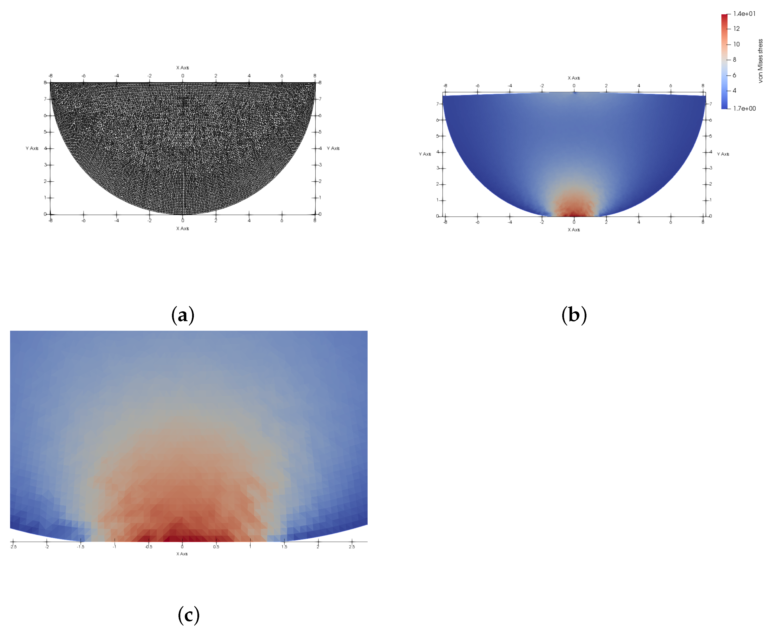
This example is adapted from [11]. The undeformed structure domain ${\Omega }_0$ is a half ball of radius R = 8 m with center $(0,R)$, and the rigid foundation is given by $\psi \left(X_1\right)=0$. The boundary ${\Gamma }_D$ is the little segment $\left[AB\right]=\{t\in (-0.095,0.095);x(t)=t,y(t)=R\}$, ${\Gamma }_C$ is the half of a circle $\{t\in (\pi ,2\pi );x(t)=Rcos(t),y(t)=R+Rsin(t\left)\right\}$, and ${\Gamma }_N$ is the rest of $\partial {\Omega }_0$.

On ${\Gamma }_D$ we impose zero horizontal displacement, in ${\Omega }_0$ volume forces $\mathbf{f}=(0,0)$ Pa/m${}^3$ are applied, and surface loads $\mathbf{h}=(h_1,h_2)=(0,-2)$ Pa/m${}^2$ are applied on ${\Gamma }_N$. We set Young’s modulus $E=150$ Pa and Poisson’s ratio $\nu =0.3$. The structure verifies the linear elasticity equation; the stress tensor of the structure written in the Lagrangian framework is $\sigma \left(\mathbf{u}\right)=\lambda \left({\nabla }_{\mathbf{X}}·\mathbf{u}\right)\mathbf{I}+2\mu {ϵ}_{\mathbf{X}}\left(\mathbf{u}\right)$, where $\lambda ,\mu >0$ are the Lamé coefficients, ${ϵ}_{\mathbf{X}}\left(\mathbf{u}\right)=\frac{1}{2}\left({\nabla }_{\mathbf{X}}\mathbf{u}+{\left({\nabla }_{\mathbf{X}}\mathbf{u}\right)}^T\right)$. In this case, the bi-linear form a and the linear form ℓ are given by

$$a\left(\mathbf{u},\mathbf{w}\right)={\int }_{{\Omega }_0}\left(\lambda \left({\nabla }_{\mathbf{X}}·\mathbf{u}\right)\left({\nabla }_{\mathbf{X}}·\mathbf{w}\right)+2\mu {ϵ}_{\mathbf{X}}\left(\mathbf{u}\right):{ϵ}_{\mathbf{X}}\left(\mathbf{w}\right)\right)d\mathbf{X}$$

and

$$\ell \left(\mathbf{w}\right)={\int }_{{\Omega }_0}\mathbf{f}·\mathbf{w}d\mathbf{X}+{\int }_{{\Gamma }_N}\mathbf{h}·\mathbf{w}ds$$

and the increment number is just $N=1$.

The quadratic optimization problem with affine constraints is

$$\mathbf{u}\in arg\underset{\mathbf{w}\in \mathbb{K}}{inf}I\left(\mathbf{w}\right)=\frac{1}{2}a(\mathbf{w},\mathbf{w})-\ell \left(\mathbf{w}\right)$$

where

$$\begin{array}{ccc}\hfill \mathbb{K}& =& \left\{\mathbf{w}:{\Omega }_0\to {\mathbb{R}}^2;\mathbf{w}={\mathbf{U}}_D on\Gamma {\Gamma }_D,\right.\hfill \\ & & \left.{\psi }^{\prime }\left(X_1\right)w_1\left(\mathbf{X}\right)-w_2\left(\mathbf{X}\right)\le X_2-\psi \left(X_1\right) on\Gamma {\Gamma }_C\right\}.\hfill \end{array}$$

The analytical normal stress in the contact zone given by the Hertz theory is

$$\left(\sigma \mathbf{n}\right)·\mathbf{n}=-\frac{4R|h_2|}{\pi b^2}\sqrt{b^2-x_1^2},\mathrm{if}\left|x_1\right|<b,\mathrm{where}b=2\sqrt{\frac{2R^2\left|h_2\right|(1-{\nu }^2)}{E\pi }}.$$

The contact zone is $|x_1|<b$ and $x_2=0$.

The number of nodes on ${\Gamma }_C$ is 252; the mesh of ${\Omega }_0$ has 11,759 vertices and 23,096 triangles. For $h_2=-2$ and $x_1=0$, the analytical value for b is $1.40621$ and for the normal stress is $-14.4871$, while the computed normal stress is $-14.545$. In Figure 1, we can see: the initial mesh, the von Mises stress and a zoom of the contact zone. The numerical solution is consistent with the analytical solution. The IPOPT algorithm solves the optimization problem after 10 iterations.

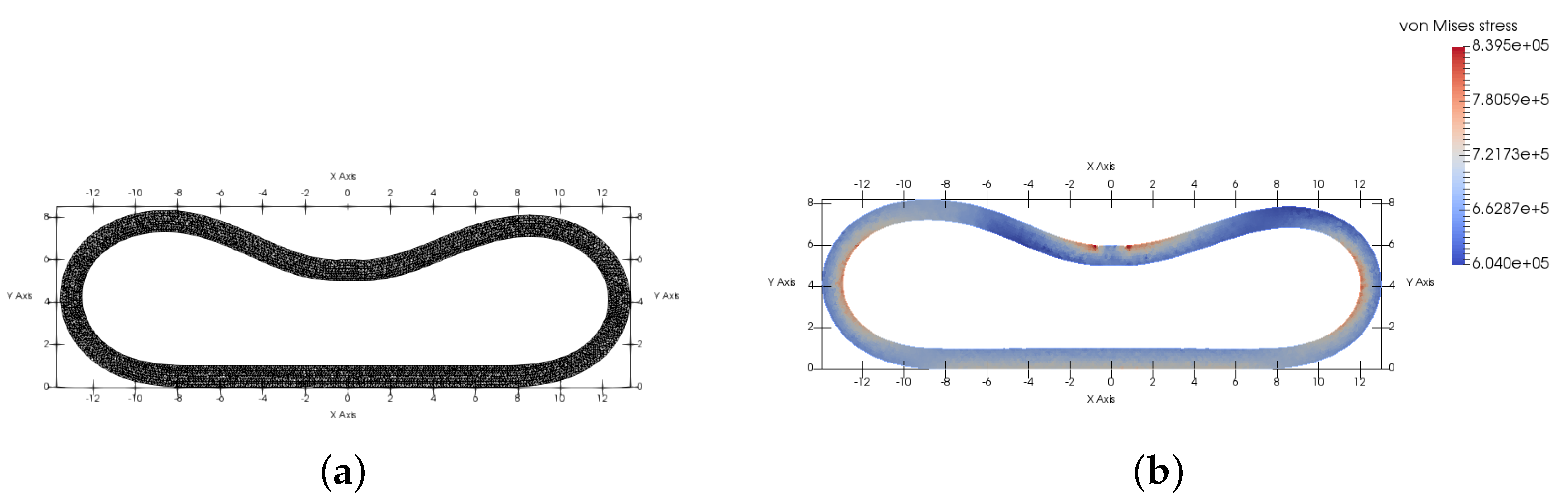
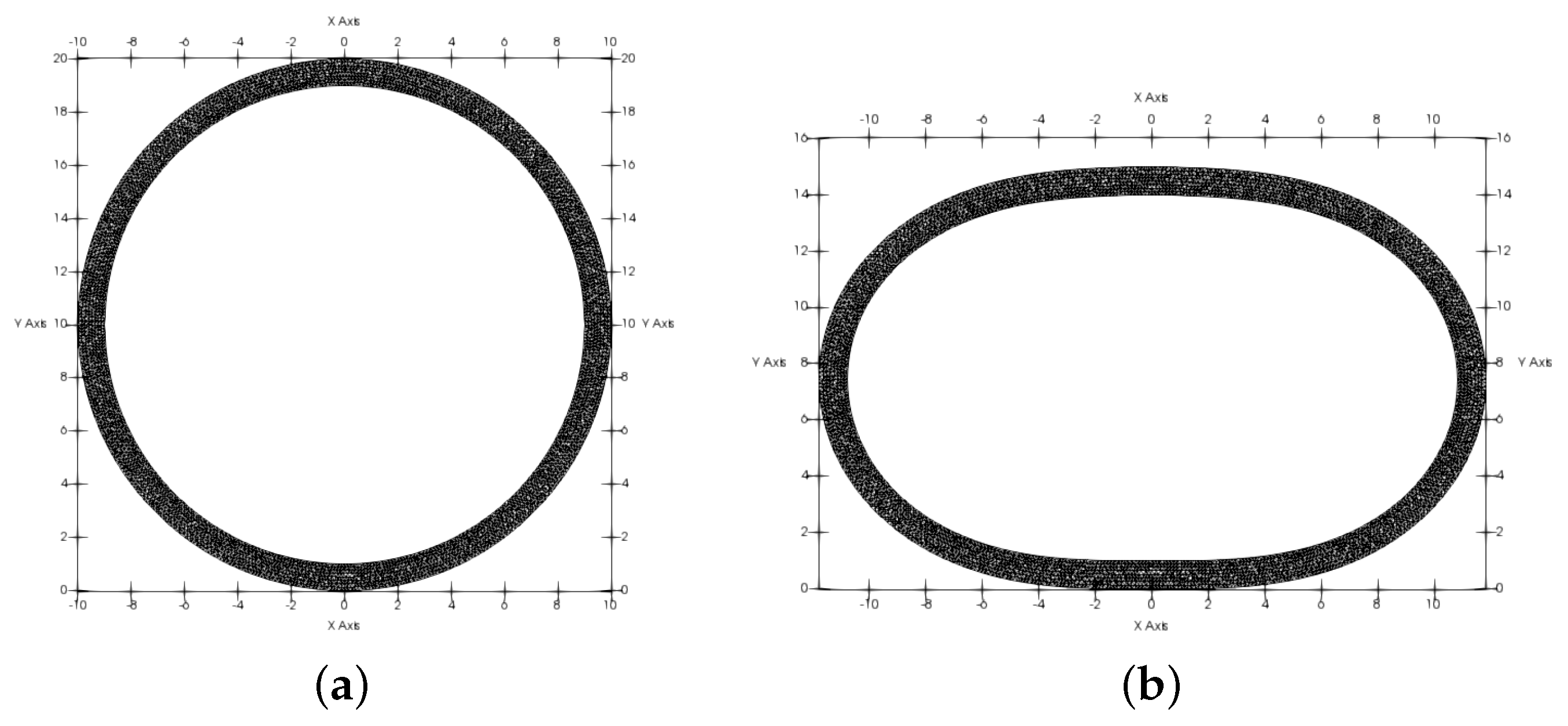
5.2. Compression of a Hyperelastic Ring against a Flat Rigid Foundation

This example is adapted from [11]. The undeformed structure domain ${\Omega }_0$ is a ring of exterior radius $R_e$ = 10 m, interior radius $R_i$ = 9 m and center $(0,R_e)$, and the rigid foundation is given by $\psi \left(X_1\right)=0$. The boundary ${\Gamma }_D$ is the arc of a circle $\stackrel{⌢}{AB}=\{t\in (\frac{\pi }{2}-\frac{\pi }{48},\frac{\pi }{2}+\frac{\pi }{48});x\left(t\right)=R_{e}cos\left(t\right),y\left(t\right)=R_e+R_{e}sin\left(t\right)\}$, ${\Gamma }_C$ is the inferior half of a circle $\{t\in (\pi ,2\pi );x\left(t\right)=R_{e}cos\left(t\right),y\left(t\right)=R_e+R_{e}sin\left(t\right)\}$, and ${\Gamma }_N$ is the rest of $\partial {\Omega }_0$.

On ${\Gamma }_D$, we impose displacement ${\mathbf{U}}_D=(0,-14)$ m, in ${\Omega }_0$, volume forces $\mathbf{f}=(0,0)$ Pa/m${}^3$ are applied, and surface loads $\mathbf{h}=(0,0)$ Pa/m${}^2$ are applied on ${\Gamma }_N$.

For the Neo-Hookean material, we use Young’s modulus $E=1.0$ MPa and Poisson’s ratio $\nu =0.45$, which gives the Lamé constants $\lambda =3.10345$ MPa and $\mu$ = 344,828 Pa. For the Ogden-like material, we use, as in [11], $c_1=0.5$ MPa, $c_2=0.5\times {10}^{-2}$ MPa, a = 0.35 MPa.

The number of nodes on ${\Gamma }_C$ is 240; the mesh of ${\Omega }_0$ has 4342 vertices and 7734 triangles. We employ finite element ${\mathbb{P}}_1$, and we set $N=14$ as the number of increments. The average number of iterations of the IPOPT algorithm in order to solve, at each increment, the optimization problem is 12.

We can see in Figure 2 the final mesh and the von Mises stress for Neo-Hookean-like material, and in Figure 3 the initial, intermediate and final meshes for the Ogden material. We denote by ${\mathbf{U}}_{nh}$ the solution in the case of the Neo-Hookean material and by ${\mathbf{U}}_{og}$ for the Ogden-like material. We have ${∥{\mathbf{U}}_{nh}-{\mathbf{U}}_{og}∥}_{L^2\left({\Omega }_0\right)}=1.88063$. Our solution for the Ogden-like material is similar to the one obtained in [11].

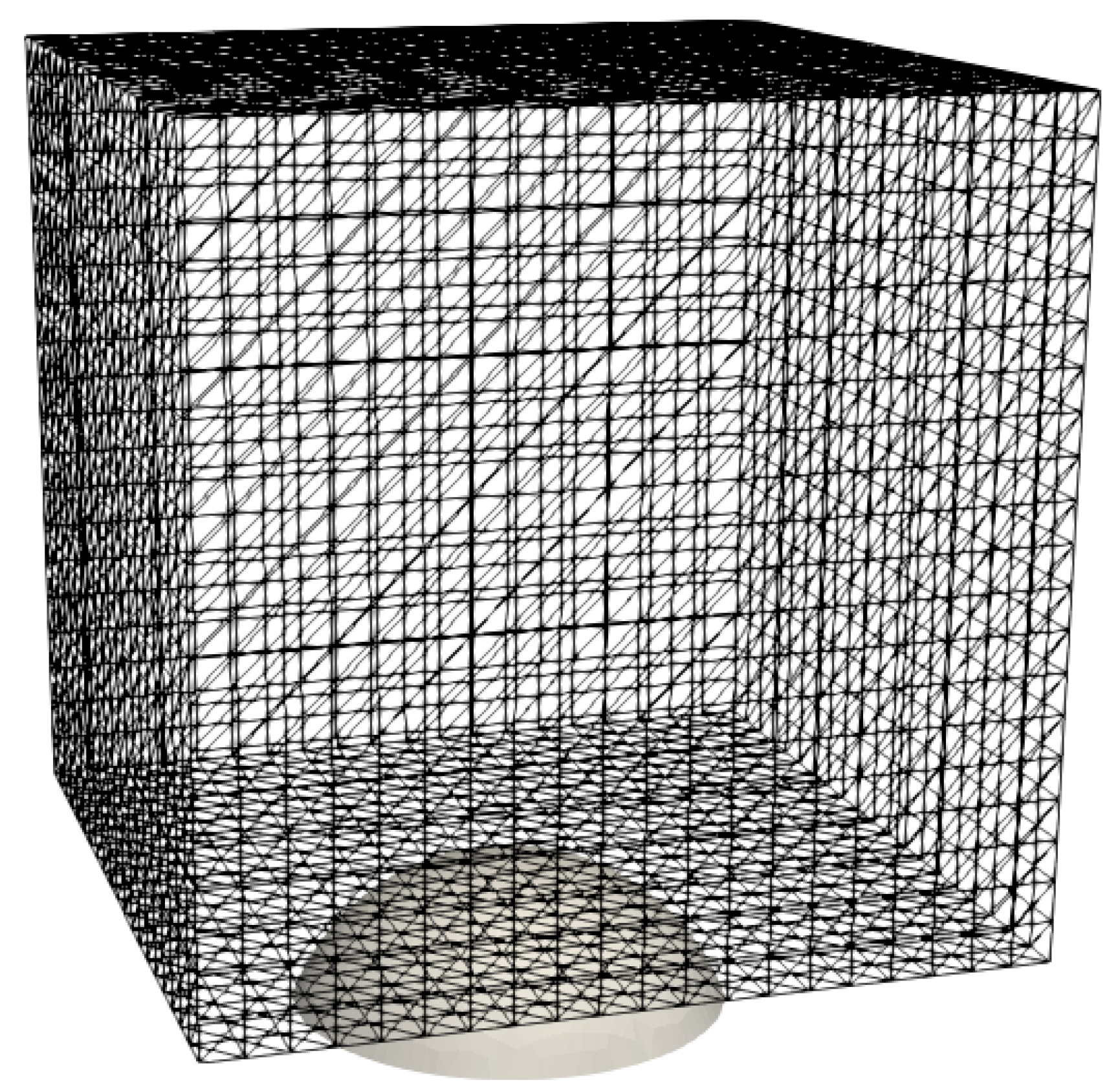
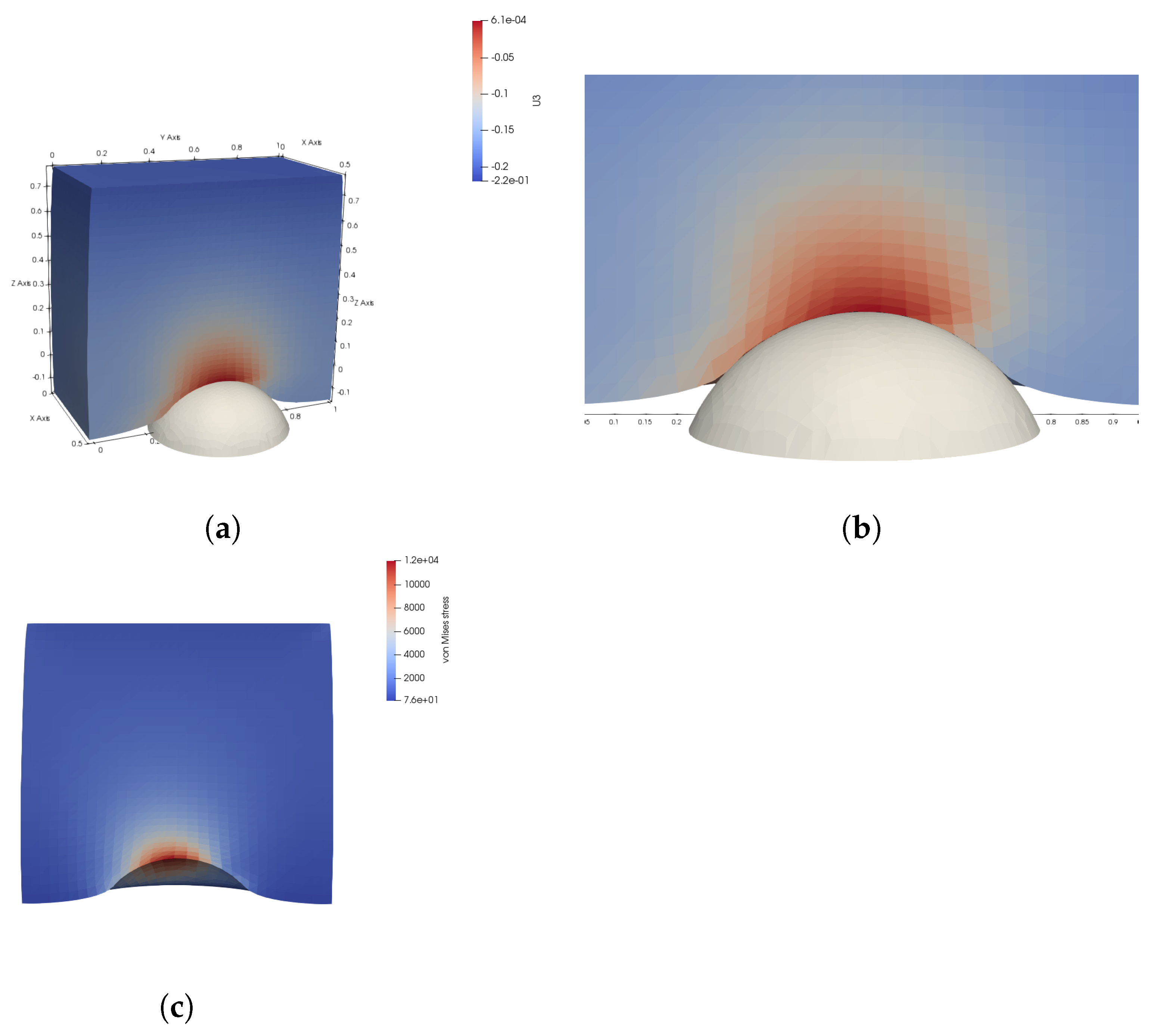
5.3. Contact of an Elastic Cube and a Ball

This example is adapted from [13]. The undeformed structure domain ${\Omega }_0$ is the cube ${(0,1)}^3$, and the obstacle is a ball with center $(0.5,0.5,-0.3)$ and radius $0.3$, see Figure 4.

The boundary ${\Gamma }_D$ is the upper side, ${\Gamma }_C$ is the bottom side, and ${\Gamma }_N$ is the rest of $\partial {\Omega }_0$. On ${\Gamma }_D$, we impose the displacement ${\mathbf{U}}_D=(0,0,-0.22)$ and we set $\mathbf{f}=(0,0,0)$ and $\mathbf{h}=(0,0,0)$. Contrary to [13], where the strain energy function is

$$\mathcal{W}=ctr\left(\mathbf{E}\right)+\frac{\lambda }{2}{\left(tr\left(\mathbf{E}\right)\right)}^2+(\mu -c)tr\left({\mathbf{E}}^2\right)-clnJ$$

with $\mathbf{E}=\frac{1}{2}\left(\mathbf{C}-\mathbf{I}\right)$ and the parameters $\lambda =5000$, $\mu =5000$, $c=1000$, we consider the Neo-Hookean material as discussed in Section 3, with Lamé constants $\lambda =5000$, $\mu =5000$.

For 3D, we have the same formula for (7), but (9) is replaced by

$$\begin{array}{ccc}\hfill \widehat{\mathbb{K}}& =& \left\{\widehat{\mathbf{w}}:\widehat{\Omega }\to {\mathbb{R}}^3;\widehat{\mathbf{w}}=\frac{1}{N}{\mathbf{U}}_{D}on{\Gamma }_D^n,\right.\hfill \\ & & \left.\frac{\partial \psi ({\widehat{x}}_1,{\widehat{x}}_2)}{\partial {\widehat{x}}_1}{\widehat{w}}_1\left(\widehat{\mathbf{x}}\right)+\frac{\partial \psi ({\widehat{x}}_1,{\widehat{x}}_2)}{\partial {\widehat{x}}_2}{\widehat{w}}_2\left(\widehat{\mathbf{x}}\right)-{\widehat{w}}_3\left(\widehat{\mathbf{x}}\right)\le {\widehat{x}}_3-\psi ({\widehat{x}}_1,{\widehat{x}}_2)on{\Gamma }_C^n\right\}.\hfill \end{array}$$

The mesh is controled by the number k of segments on each edge of the cube. The mesh of ${\Omega }_0$ has: 9261 vertices and 48,000 tetrahedrons for $k=20$, 35,937 vertices and 197,608 tetrahedrons for $k=32$ and 68,921 vertices and 384,000 tetrahedrons for $k=40$. We employ the finite element ${\mathbb{P}}_1$, and we set $N=4$ as the number of increments.

The optimization problem has

• $k=20$: 27,783 variables, 361 inequality constraints, 441 variables with imposed displacement;
• $k=32$: 107,811 variables, 961 inequality constraints, 1089 variables with imposed displacement;
• $k=40$: 206,763 variables, 1531 inequality constraints, 1681 variables with imposed displacement.

The average number of iterations of the IPOPT algorithm is 14 for $k=20$ and $16.75$ for $k=40$. The total CPU time on an Intel Sandy Bridge 16 × 3.30 GHz and 64 GB RAM was 6 min for $k=20$, 24 min for $k=32$ and 50 min for $k=40$.

We denote by ${\mathbf{U}}_{nh}^{k20}$, ${\mathbf{U}}_{nh}^{k32}$, ${\mathbf{U}}_{nh}^{k40}$ the solutions for $k=20$, $k=32$, $k=40$, respectively. The $L^2$ error between computed solutions are: ${∥{\mathbf{U}}_{nh}^{k32}-{\mathbf{U}}_{nh}^{k20}∥}_{L^2\left({\Omega }_0\right)}=0.002149$, ${∥{\mathbf{U}}_{nh}^{k40}-{\mathbf{U}}_{nh}^{k20}∥}_{L^2\left({\Omega }_0\right)}=0.002868$, ${∥{\mathbf{U}}_{nh}^{k40}-{\mathbf{U}}_{nh}^{k32}∥}_{L^2\left({\Omega }_0\right)}=0.0007273$.

In Figure 5, we plot the vertical displacement and von Mises stress at the final configuration for $k=32$.

6. Conclusions

An Updated Lagrangian method for nonlinear elasticity with frictionless contact was presented. The linearized problem written in the updated configuration for Neo-Hookean and Ogden compressible materials were derived. At each iteration, only a linear system was solved. Two- and three-dimensional numerical simulations were performed.

References

- Kikuchi, N.; Oden, J.T. Contact Problems in Elasticity: A Study of Variational Inequalities and Finite Element Methods; SIAM Studies in Applied Mathematics, 8; Society for Industrial and Applied Mathematics (SIAM): Philadelphia, PA, USA, 1988. [Google Scholar]
- Laursen, T.A. Computational Contact and Impact Mechanics. Fundamentals of Modeling Interfacial Phenomena in Nonlinear Finite Element Analysis; Springer: Berlin, Germany, 2002. [Google Scholar]
- Han, W.; Sofonea, M. Quasistatic Contact Problems in Viscoelasticity and Viscoplasticity; AMS/IP Studies in Advanced Mathematics, 30; American Mathematical Society: Providence, RI, USA; International Press: Somerville, MA, USA, 2002. [Google Scholar]
- Wriggers, P. Computational Contact Mechanics; Springer: Berlin, Germany, 2006. [Google Scholar]
- Glowinski, R.; Lions, J.-L.; Trémolières, R. Analyse Numérique des Inéquations Variationnelles. Tome 1. Théorie Générale Premiéres Applications; Méthodes Mathématiques de l’Informatique, 5; Dunod: Paris, France, 1976. [Google Scholar]
- Belgacem, F.B.; Hild, P.; Laborde, P. Extension of the mortar finite element method to a variational inequality modeling unilateral contact. Math. Models Methods Appl. Sci. 1999, 9, 287–303. [Google Scholar] [CrossRef]
- Belytschko, T.; Daniel, W.J.T.; Ventura, G. A monolithic smoothing-gap algorithm for contact-impact based on the signed distance function. J. Numer. Methods Eng. 2002, 55, 101–125. [Google Scholar] [CrossRef]
- Yakhlef, O.; Murea, C.M. Numerical simulation of dynamic fluid-structure interaction with elastic structure-rigid obstacle contact. Fluids 2021, 6, 51. [Google Scholar] [CrossRef]
- Hintermuller, M.; Kovtunenko, V.; Kunish, K. Semismooth newton methods for a class of unilaterally constrained variational problems. Adv. Math. Sci. Appl. 2004, 147, 513–535. [Google Scholar]
- Krause, R. From Inexact Active Set Strategies to Nonlinear Multigrid Methods; Lecture Notes in Applied and Computational Mechanics; Springer: Berlin, Germany, 2006. [Google Scholar]
- Abide, S.; Barboteu, M.; Danan, D. Analysis of two active set type methods to solve unilateral contact problems. Appl. Math. Comput. 2016, 284, 286–307. [Google Scholar] [CrossRef]
- Abide, S.; Barboteu, M.; Cherkaoui, S.; Danan, D.; Dumont, S. Inexact primal-dual active set method for solving elastodynamic frictional contact problems. Comput. Math. Appl. 2021, 82, 36–59. [Google Scholar] [CrossRef]
- Krause, R.; Mohr, C. Level set based multi-scale methods for large deformation contact problems. Appl. Numer. Math. 2011, 61, 428–442. [Google Scholar] [CrossRef]
- Chouly, F.; Hild, P.; Renard, Y. Symmetric and non-symmetric variants of Nitsche’s method for contact problems in elasticity: Theory and numerical experiments. Math. Comp. 2015, 84, 1089–1112. [Google Scholar] [CrossRef]
- Kshirsagar, S.; Lee, C.; Natarajan, S. α-finite element method for frictionless and frictional contact including large deformation. Int. J. Comput. Methods 2021, 18, 2150002. [Google Scholar] [CrossRef]
- Poluektov, M.; Figiel, L. A cut finite-element method for fracture and contact problems in large-deformation solid mechanics. Comput. Methods Appl. Mech. Eng. 2022, 388, 114234. [Google Scholar] [CrossRef]
- Ciarlet, P.G. Mathematical Elasticity, Volume 1: Three Dimensional Elasticity; Elsevier: Amsterdam, The Netherlands, 2005. [Google Scholar]
- Belytschko, T.; Liu, W.K.; Moran, B. Nonlinear Finite Elements for Continua and Structures; John Wiley & Sons, Ltd.: Chichester, UK, 2000. [Google Scholar]
- Fortin, A.; Garon, A. Les Eléments Finis: De la Théorie à la Pratique; Université Laval: Québec, QC, Canada, 2016. [Google Scholar]
- Murea, C.M.; Sy, S. Updated Lagrangian/Arbitrary Lagrangian Eulerian framework for interaction between a compressible Neo-Hookean structure and an incompressible fluid. Internat. J. Numer. Methods Eng. 2017, 103, 1067–1084. [Google Scholar] [CrossRef]
- Murea, C.M. Stable semi-implicit monolithic scheme for interaction between incompressible neo-Hookean structure and Navier-Stokes fluid. J. Math. Study 2019, 52, 448–469. [Google Scholar]
- Holzapfel, G.A. Nonlinear Solid Mechanics. A Continuum Approach for Engineering; John Wiley & Sons, Ltd.: Chichester, UK, 2000. [Google Scholar]
- Bonet, J.; Wood, R.D. Nonlinear Continuum Mechanics for Finite Element Analysis; Cambridge University Press: Cambridge, UK, 2008. [Google Scholar]
- Hecht, F. New development in freefem++. J. Numer. Math. 2012, 20, 251–265. [Google Scholar] [CrossRef]
- Ogden, R.W. Large deformation isotropic elasticity: On the correlation of theory and experiment for compressible rubberlike solids. Proc. R. Soc. Lond. A 1972, 328, 567–583. [Google Scholar] [CrossRef]
- Ciarlet, P.G.; Geymonat, G. Sur les lois de comportement en élasticité non-linéaire compressible. Comptes Rendus Acad. Sci. 1982, 295, 423–426. [Google Scholar]
Figure 1.
Hertz half ball: the undeformed mesh (a), the von Mises stress after compression (b) and a zoom of the contact zone (c).
Figure 2.
Ring, Neo-Hookean model: mesh deformation (a) and von Mises stress (b) after 14 increments.
Figure 3.
Ring, Ogden model: mesh deformation after: 0 (a), 5 (b), 10 (c) and 14 (d) increments.
Figure 4.
Cube: initial configuration.
Figure 5.
Cube, , cut of the final configuration: vertical displacement (a), zoom of the contact zone for (b), von Mises stress (c).
Publisher’s Note: MDPI stays neutral with regard to jurisdictional claims in published maps and institutional affiliations. |
© 2022 by the author. Licensee MDPI, Basel, Switzerland. This article is an open access article distributed under the terms and conditions of the Creative Commons Attribution (CC BY) license (https://creativecommons.org/licenses/by/4.0/).
Share and Cite
MDPI and ACS Style
Murea, C.M. Updated Lagrangian for Compressible Hyperelastic Material with Frictionless Contact. Appl. Mech. 2022, 3, 533-543. https://doi.org/10.3390/applmech3020031
AMA Style
Murea CM. Updated Lagrangian for Compressible Hyperelastic Material with Frictionless Contact. Applied Mechanics. 2022; 3(2):533-543. https://doi.org/10.3390/applmech3020031
Chicago/Turabian StyleMurea, Cornel Marius. 2022. "Updated Lagrangian for Compressible Hyperelastic Material with Frictionless Contact" Applied Mechanics 3, no. 2: 533-543. https://doi.org/10.3390/applmech3020031