

Training Artificial Neural Networks Using a Global Optimization Method That Utilizes Neural Networks


Abstract
:1. Introduction
2. The Proposed Method
2.1. Preliminaries
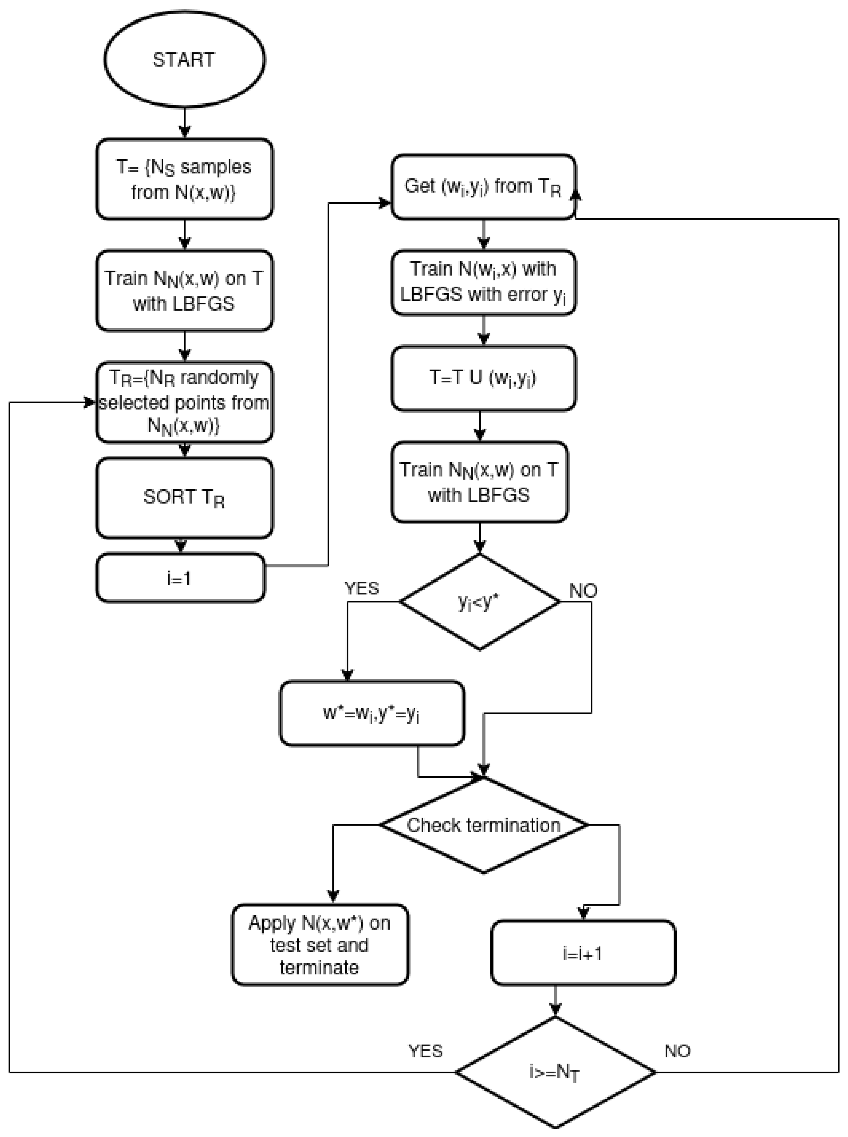
2.2. The Modified NeuralMinimizer Method
- Initialization step.
- (a)
- SetH the number of weights of the neural network. In the current method the same number of weights was used for both and artificial neural networks.
- (b)
- Set as the samples that will be initially drawn from . At this stage, the training error for the artificial neural network will be used as an objective function to minimize
- (c)
- Set as the number of points that will be utilized as local minimization method starters in every iteration.
- (d)
- Set as the number of samples that will be drawn from the network in each iteration.
- (e)
- Set as the maximum number of iterations allowed.
- (f)
- Set Iter = 0, the current iteration number.
- (g)
- Set as the global minimum discovered by the method. Initially
- Creation Step.
- (a)
- Set , the used training set for the neural network.
- (b)
- For do
- Draw a new sample from .
- Calculate using Equation 1
- (c)
- EndFor
- (d)
- Train the neural network on set T using the L-BFGS method.
- Sampling Step
- (a)
- Set
- (b)
- For do
- Produce randomly a sample from neural network
- Set
- (c)
- EndFor
- (d)
- Sort in ascending with respect to the values
- Optimization Step.
- (a)
- For do
- Get the next item from .
- Train the neural network on the training set of the objective problem using the L-BFGS method and obtain the corresponding training error .
- Update
- Train the network again on the modified set T. In this step, the original training set used by is updated to include the new discovered local minimum. This operation is used in order to construct a more accurate approximation of the real objective function.
- If then
- If the termination rule proposed in [95], then apply the produced network on the test set of the objective problem, report the test error and terminate.
- (b)
- EndFor
- Set iter=iter+1
- Goto to Sampling step.
3. Experiments
- The UCI repository, https://archive.ics.uci.edu/ (accessed on 12 July 2023) [96]
- The Keel repository, https://sci2s.ugr.es/keel/datasets.php (accessed on 17 June 2023) [97].
- The Statlib URL ftp://lib.stat.cmu.edu/datasets/index.html (accessed on 17 June 2023). This repository is used mainly for the regression datasets.
3.1. Experimental Datasets
- Australian dataset [100], an economic dataset, related to bank transactions.
- Balance dataset [101], which is related to psychological experiments.
- Bands dataset, related to printing problems [104].
- Dermatology dataset [105], a dataset related to dermatology problems.
- Hayes-Roth dataset [106].
- Heart dataset [107], a medical dataset used to detect heart diseases.
- HouseVotes dataset [108], related to the Congressional voting records of USA.
- Lymography dataset [113].
- Mammographic dataset [114], a medical dataset related to breast cancer diagnosis.
- Page Blocks dataset [115].
- Pima dataset [118], a medical dataset.
- Popfailures dataset [119], a dataset related to meteorological data.
- Regions2 dataset, a medical dataset for liver biopsy images [120].
- Saheart dataset [121], a medical dataset related to heart diseases.
- Segment dataset [122], a dataset related to image segmentation.
- Wdbc dataset [123], a dataset related to breast tumors.
- (a)
- Z_F_S,
- (b)
- ZO_NF_S
- (c)
- ZONF_S.
- Zoo dataset [128], suggested for the detection of the proper classes of animals.
- Abalone dataset [129], proposed to predict the age of abalones.
- Airfoil dataset, a dataset provided by NASA [130], created from a series of aerodynamic and acoustic tests.
- Baseball dataset, a dataset using baseball games.
- BK dataset [131], used to predict the points scored in a basketball game.
- BL dataset, used in machine problems.
- Concrete dataset [132], a dataset proposed to calculate the compressive strength of concrete.
- Dee dataset, used to detect the electricity energy prices.
- Diabetes dataset, a medical dataset.
- Housing dataset [133].
- FA dataset, used to fit body fat to other measurements.
- MB dataset [131].
- Mortgage dataset. The goal is to predict the 30-year conventional mortgage rate.
- PY dataset, (pyrimidines problem) [134].
- Quake dataset, used to approximate the strength of a earthquake given its the depth of its focal point, its latitude and its longitude.
- Treasure dataset, which contains economic data information from the USA, where the goal is to predict the 1-month CD Rate.
- Wankara dataset, a weather dataset.
3.2. Experimental Setup
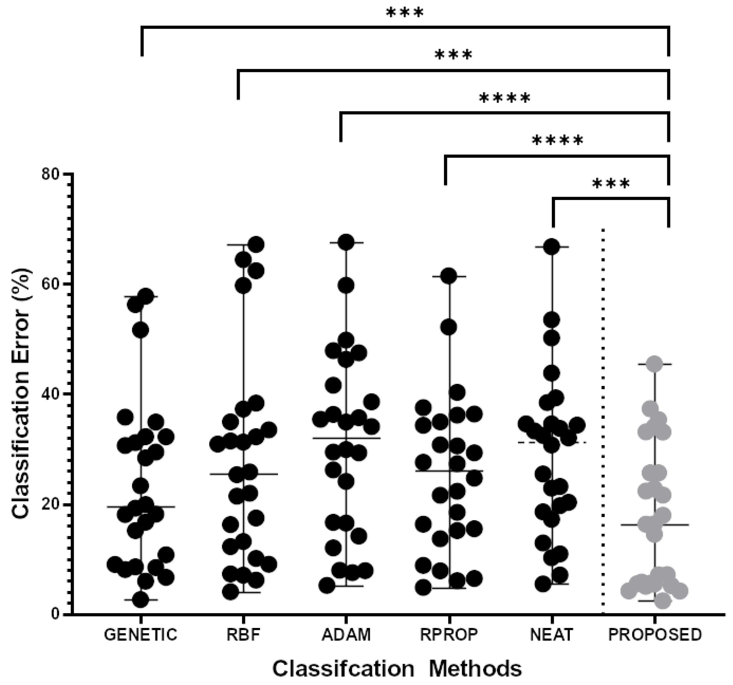
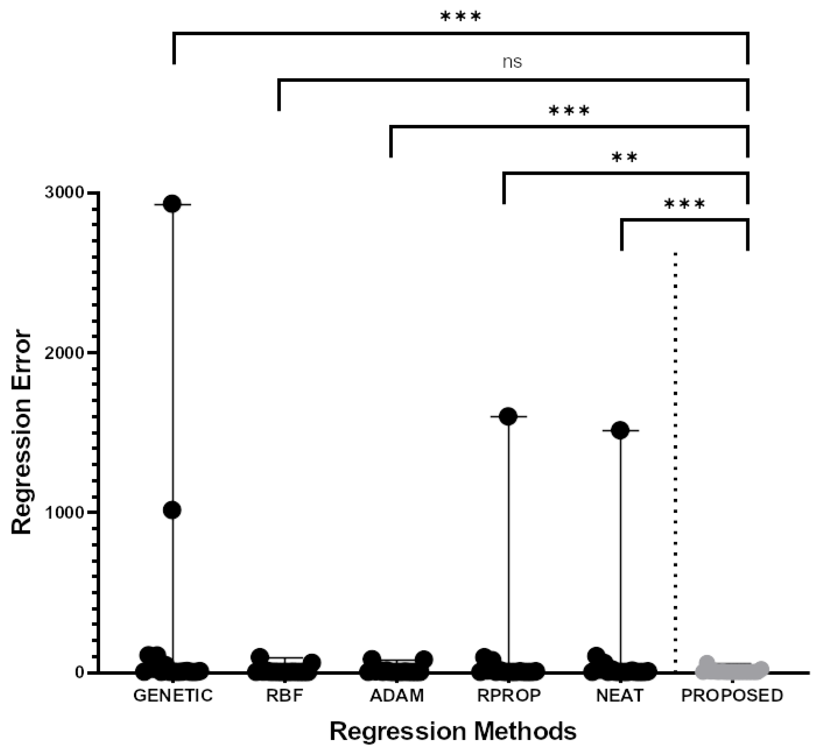
- A genetic algorithm with 200 chromosomes was used to train a neural network with H hidden nodes. This method was denoted as GENETIC in the tables holding the experimental results.
- A radial basis function (RBF) network [78] with H hidden nodes.
- The Adam optimization method [84]. Here, the method was used to minimize the train error of a neural network with H hidden nodes.
- The NEAT method (NeuroEvolution of Augmenting Topologies ) [135].
3.3. Experimental Results
4. Conclusions
Author Contributions
Funding
Institutional Review Board Statement
Informed Consent Statement
Data Availability Statement
Acknowledgments
Conflicts of Interest
References
- Bishop, C. Neural Networks for Pattern Recognition; Oxford University Press: Oxford, UK, 1995. [Google Scholar]
- Cybenko, G. Approximation by superpositions of a sigmoidal function. Math. Control. Signals Syst. 1989, 2, 303–314. [Google Scholar] [CrossRef]
- Abiodun, O.I.; Jantan, A.; Omolara, A.E.; Dada, K.V.; Mohamed, N.A.; Arshad, H. State-of-the-art in artificial neural network applications: A survey. Heliyon 2018, 4, e00938. [Google Scholar] [CrossRef] [PubMed] [Green Version]
- Baldi, P.; Cranmer, K.; Faucett, T.; Sadowski, P.; Whiteson, D. Parameterized neural networks for high-energy physics. Eur. Phys. J. C 2016, 76, 235. [Google Scholar] [CrossRef] [Green Version]
- Valdas, J.J.; Bonham-Carter, G. Time dependent neural network models for detecting changes of state in complex processes: Applications in earth sciences and astronomy. Neural Netw. 2006, 19, 196–207. [Google Scholar] [CrossRef] [PubMed]
- Carleo, G.; Troyer, M. Solving the quantum many-body problem with artificial neural networks. Science 2017, 355, 602–606. [Google Scholar] [CrossRef] [Green Version]
- Shen, L.; Wu, J.; Yang, W. Multiscale Quantum Mechanics/Molecular Mechanics Simulations with Neural Networks. J. Chem. Theory Comput. 2016, 12, 4934–4946. [Google Scholar] [CrossRef]
- Manzhos, S.; Dawes, R.; Carrington, T. Neural network-based approaches for building high dimensional and quantum dynamics-friendly potential energy surfaces. Int. J. Quantum Chem. 2015, 115, 1012–1020. [Google Scholar] [CrossRef] [Green Version]
- Wei, J.N.; Duvenaud, D.; Aspuru-Guzik, A. Neural Networks for the Prediction of Organic Chemistry Reactions. ACS Cent. Sci. 2016, 2, 725–732. [Google Scholar] [CrossRef]
- Falat, L.; Pancikova, L. Quantitative Modelling in Economics with Advanced Artificial Neural Networks. Procedia Econ. Financ. 2015, 34, 194–201. [Google Scholar] [CrossRef] [Green Version]
- Namazi, M.; Shokrolahi, A.; Maharluie, M.S. Detecting and ranking cash flow risk factors via artificial neural networks technique. J. Bus. Res. 2016, 69, 1801–1806. [Google Scholar] [CrossRef]
- Tkacz, G. Neural network forecasting of Canadian GDP growth. Int. J. Forecast. 2001, 17, 57–69. [Google Scholar] [CrossRef]
- Baskin, I.I.; Winkler, D.; Tetko, I.V. A renaissance of neural networks in drug discovery. Expert Opin. Drug Discov. 2016, 11, 785–795. [Google Scholar] [CrossRef] [PubMed]
- Bartzatt, R. Prediction of Novel Anti-Ebola Virus Compounds Utilizing Artificial Neural Network (ANN). World J. Pharm. Res. 2018, 7, 16. [Google Scholar]
- Lagaris, I.E.; Likas, A.; Fotiadis, D.I. Artificial neural networks for solving ordinary and partial differential equations. IEEE Trans. Neural Netw. 1998, 9, 987–1000. [Google Scholar] [CrossRef] [PubMed] [Green Version]
- Effati, S.; Pakdaman, M. Artificial neural network approach for solving fuzzy differential equations. Inf. Sci. 2010, 180, 1434–1457. [Google Scholar] [CrossRef]
- Rostami, F.; Jafarian, A. A new artificial neural network structure for solving high-order linear fractional differential equations. Int. J. Comput. Math. 2018, 95, 528–539. [Google Scholar] [CrossRef]
- Yadav, A.K.; Chandel, S.S. Solar radiation prediction using Artificial Neural Network techniques: A review. Renew. Sustain. Energy Rev. 2014, 33, 772–781. [Google Scholar] [CrossRef]
- Qazi, A.; Fayaz, H.; Wadi, A.; Raj, R.G.; Rahim, N.A.; Khan, W.A. The artificial neural network for solar radiation prediction and designing solar systems: A systematic literature review. J. Clean. Prod. 2015, 104, 1–12. [Google Scholar] [CrossRef]
- Wu, C.H. Behavior-based spam detection using a hybrid method of rule-based techniques and neural networks. Expert Syst. Appl. 2009, 36, 4321–4330. [Google Scholar] [CrossRef]
- Ren, Y.; Ji, D. Neural networks for deceptive opinion spam detection: An empirical study. Inf. Sci. 2017, 385–386, 213–224. [Google Scholar] [CrossRef]
- Madisetty, S.; Desarkar, M.S. A Neural Network-Based Ensemble Approach for Spam Detection in Twitter. IEEE Trans. Comput. Soc. Syst. 2018, 5, 973–984. [Google Scholar] [CrossRef]
- Topuz, A. Predicting moisture content of agricultural products using artificial neural networks. Adv. Eng. 2010, 41, 464–470. [Google Scholar] [CrossRef]
- Escamilla-García, A.; Soto-Zarazúa, G.M.; Toledano-Ayala, M.; Rivas-Araiza, E.; Gastélum-Barrios, A. Applications of Artificial Neural Networks in Greenhouse Technology and Overview for Smart Agriculture Development. Appl. Sci. 2020, 10, 3835. [Google Scholar] [CrossRef]
- Boughrara, H.; Chtourou, M.; Ben Amar, C.; Chen, L. Facial expression recognition based on a mlp neural network using constructive training algorithm. Multimed. Tools Appl. 2016, 75, 709–731. [Google Scholar] [CrossRef]
- Liu, H.; Tian, H.Q.; Li, Y.F.; Zhang, L. Comparison of four Adaboost algorithm based artificial neural networks in wind speed predictions. Energy Convers. Manag. 2015, 92, 67–81. [Google Scholar] [CrossRef]
- Szoplik, J. Forecasting of natural gas consumption with artificial neural networks. Energy 2015, 85, 208–220. [Google Scholar] [CrossRef]
- Bahram, H.; Navimipour, N.J. Intrusion detection for cloud computing using neural networks and artificial bee colony optimization algorithm. ICT Express 2019, 5, 56–59. [Google Scholar]
- Chen, Y.S.; Chang, F.J. Evolutionary artificial neural networks for hydrological systems forecasting. J. Hydrol. 2009, 367, 125–137. [Google Scholar] [CrossRef]
- Swales, G.S.; Yoon, Y. Applying Artificial Neural Networks to Investment Analysis. Financ. Anal. J. 1992, 48, 78–80. [Google Scholar] [CrossRef]
- Rumelhart, D.E.; Hinton, G.E.; Williams, R.J. Learning representations by back-propagating errors. Nature 1986, 323, 533–536. [Google Scholar] [CrossRef]
- Chen, T.; Zhong, S. Privacy-Preserving Backpropagation Neural Network Learning. IEEE Trans. Neural Netw. 2009, 20, 1554–1564. [Google Scholar] [CrossRef] [PubMed]
- Chalup, S.; Maire, F. A study on hill climbing algorithms for neural network training. In Proceedings of the 1999 Congress on Evolutionary Computation-CEC99 (Cat. No. 99TH8406), Washington, DC, USA, 6–9 July 1999; IEEE: Toulouse, France, 1999; Volume 3, pp. 2014–2021. [Google Scholar]
- Riedmiller, M.; Braun, H. A Direct Adaptive Method for Faster Backpropagation Learning: The RPROP algorithm. In Proceedings of the IEEE International Conference on Neural Networks, San Francisco, CA, USA, 28 March–1 April 1993; IEEE: Toulouse, France, 1993; pp. 586–591. [Google Scholar]
- Pajchrowski, T.; Zawirski, K.; Nowopolski, K. Neural Speed Controller Trained Online by Means of Modified RPROP Algorithm. IEEE Trans. Ind. Informatics 2015, 11, 560–568. [Google Scholar] [CrossRef]
- Hermanto, R.P.S.; Nugroho, A. Waiting-Time Estimation in Bank Customer Queues using RPROP Neural Networks. Procedia Comput. Sci. 2018, 135, 35–42. [Google Scholar] [CrossRef]
- Robitaille, B.; Marcos, B.; Veillette, M.; Payre, G. Modified quasi-Newton methods for training neural networks. Comput. Chem. Eng. 1996, 20, 1133–1140. [Google Scholar] [CrossRef]
- Liu, Q.; Liu, J.; Sang, R.; Li, J.; Zhang, T.; Zhang, Q. Fast Neural Network Training on FPGA Using Quasi-Newton Optimization Method. IEEE Trans. Very Large Scale Integr. (VLSI) Syst. 2018, 26, 1575–1579. [Google Scholar] [CrossRef]
- Yamazaki, A.; de Souto, M.C.P.; Ludermir, T.B. Optimization of neural network weights and architectures for odor recognition using simulated annealing. In Proceedings of the 2002 International Joint Conference on Neural Networks, IJCNN’02, Honolulu, HI, USA, 12–17 May 2002; IEEE: Toulouse, France, 2002; Volume 1, pp. 547–552. [Google Scholar]
- Da, Y.; Xiurun, G. An improved PSO-based ANN with simulated annealing technique. Neurocomputing 2005, 63, 527–533. [Google Scholar] [CrossRef]
- Leung, F.H.F.; Lam, H.K.; Ling, S.H.; Tam, P.K.S. Tuning of the structure and parameters of a neural network using an improved genetic algorithm. IEEE Trans. Neural Netw. 2003, 14, 79–88. [Google Scholar] [CrossRef] [Green Version]
- Yao, X. Evolving artificial neural networks. Proc. IEEE 1999, 87, 1423–1447. [Google Scholar]
- Zhang, C.; Shao, H.; Li, Y. Particle swarm optimisation for evolving artificial neural network. In Proceedings of the IEEE International Conference on Systems, Man, and Cybernetics, Nashville, TN, USA, 8–11 October 2000; IEEE: Toulouse, France, 2000; pp. 2487–2490. [Google Scholar]
- Yu, J.; Wang, S.; Xi, L. Evolving artificial neural networks using an improved PSO and DPSO. Neurocomputing 2008, 71, 1054–1060. [Google Scholar] [CrossRef]
- Ilonen, J.; Kamarainen, J.K.; Lampinen, J. Differential Evolution Training Algorithm for Feed-Forward Neural Networks. Neural Process. Lett. 2003, 17, 93–105. [Google Scholar] [CrossRef]
- Slowik, A.; Bialko, M. Training of artificial neural networks using differential evolution algorithm. In Proceedings of the 2008 Conference on Human System Interactions, Krakow, Poland, 25–27 May 2008; IEEE: Toulouse, France, 2008; pp. 60–65. [Google Scholar]
- Rocha, M.; Cortez, P.; Neves, J. Evolution of neural networks for classification and regression. Neurocomputing 2007, 70, 2809–2816. [Google Scholar] [CrossRef] [Green Version]
- Aljarah, I.; Faris, H.; Mirjalili, S. Optimizing connection weights in neural networks using the whale optimization algorithm. Soft Comput. 2018, 22, 1–15. [Google Scholar] [CrossRef]
- Askarzadeh, A.; Rezazadeh, A. Artificial neural network training using a new efficient optimization algorithm. Appl. Soft Comput. 2013, 13, 1206–1213. [Google Scholar] [CrossRef]
- Cui, Z.; Yang, C.; Sanyal, S. Training artificial neural networks using APPM. Int. J. Wirel. And Mobile Comput. 2012, 5, 168–174. [Google Scholar] [CrossRef] [Green Version]
- Yaghini, M.; Khoshraftar, M.M.; Fallahi, M. A hybrid algorithm for artificial neural network training. Eng. Appl. Artif. Intell. 2013, 26, 293–301. [Google Scholar] [CrossRef]
- Chen, J.F.; Do, Q.H.; Hsieh, H.N. Training Artificial Neural Networks by a Hybrid PSO-CS Algorithm. Algorithms 2015, 8, 292–308. [Google Scholar] [CrossRef] [Green Version]
- Yang, X.S.; Deb, S. Engineering Optimisation by Cuckoo Search. Int. J. Math. Model. Numer. Optim. 2010, 1, 330–343. [Google Scholar] [CrossRef]
- Ivanova, I.; Kubat, M. Initialization of neural networks by means of decision trees. Knowl.-Based Syst. 1995, 8, 333–344. [Google Scholar] [CrossRef]
- Yam, J.Y.F.; Chow, T.W.S. A weight initialization method for improving training speed in feedforward neural network. Neurocomputing 2000, 30, 219–232. [Google Scholar] [CrossRef]
- Chumachenko, K.; Iosifidis, A.; Gabbouj, M. Feedforward neural networks initialization based on discriminant learning. Neural Netw. 2022, 146, 220–229. [Google Scholar] [CrossRef]
- Itano, F.; de Sousa, M.A.d.A.; Del-Moral-Hernandez, E. Extending MLP ANN hyper-parameters Optimization by using Genetic Algorithm. In Proceedings of the 2018 International Joint Conference on Neural Networks (IJCNN), Rio de Janeiro, Brazil, 8–13 July 2018; IEEE: Toulouse, France, 2018; pp. 1–8. [Google Scholar]
- Narkhede, M.V.; Bartakke, P.P.; Sutaone, M.S. A review on weight initialization strategies for neural networks. Artif. Intell. Rev. 2022, 55, 291–322. [Google Scholar] [CrossRef]
- O’Neill, M.; Ryan, C. Grammatical evolution. IEEE Trans. Evol. Comput. 2001, 5, 349–358. [Google Scholar] [CrossRef] [Green Version]
- Tsoulos, I.G.; Gavrilis, D.; Glavas, E. Neural network construction and training using grammatical evolution. Neurocomputing 2008, 72, 269–277. [Google Scholar] [CrossRef]
- Han, H.G.; Qiao, J.F. A structure optimisation algorithm for feedforward neural network construction. Neurocomputing 2013, 99, 347–357. [Google Scholar] [CrossRef]
- Kim, K.J.; Cho, S.B. Evolved neural networks based on cellular automata for sensory-motor controller. Neurocomputing 2006, 69, 2193–2207. [Google Scholar] [CrossRef]
- Martínez-Zarzuela, M.; Díaz Pernas, F.J.; Díez Higuera, J.F.; Rodríguez, M.A. Fuzzy ART Neural Network Parallel Computing on the GPU. In Computational and Ambient Intelligence. IWANN 2007; Lecture Notes in Computer Science; Sandoval, F., Prieto, A., Cabestany, J., Graña, M., Eds.; Springer: Berlin/Heidelberg, Germany, 2007; Volume 4507. [Google Scholar]
- Sierra-Canto, X.; Madera-Ramirez, F.; Uc-Cetina, V. Parallel Training of a Back-Propagation Neural Network Using CUDA. In Proceedings of the 2010 Ninth International Conference on Machine Learning and Applications, Washington, DC, USA, 12–14 December 2010; IEEE: Toulouse, France, 2010; pp. 307–312. [Google Scholar]
- Huqqani, A.A.; Schikuta, E.; Chen, S.Y.P. Multicore and GPU Parallelization of Neural Networks for Face Recognition. Procedia Comput. Sci. 2013, 18, 349–358. [Google Scholar] [CrossRef] [Green Version]
- Nowlan, S.J.; Hinton, G.E. Simplifying neural networks by soft weight sharing. Neural Comput. 1992, 4, 473–493. [Google Scholar] [CrossRef]
- Kim, J.K.; Lee, M.Y.; Kim, J.Y.; Kim, B.J.; Lee, J.H. An efficient pruning and weight sharing method for neural network. In Proceedings of the 2016 IEEE International Conference on Consumer Electronics-Asia (ICCE-Asia), Seoul, Republic of Korea, 26–28 October 2016; IEEE: Toulouse, France, 2016; pp. 1–2. [Google Scholar]
- Hanson, S.J.; Pratt, L.Y. Comparing biases for minimal network construction with back propagation. In Advances in Neural Information Processing Systems; Touretzky, D.S., Ed.; Morgan Kaufmann: San Mateo, CA, USA, 1989; Volume 1, pp. 177–185. [Google Scholar]
- Mozer, M.C.; Smolensky, P. Skeletonization: A technique for trimming the fat from a network via relevance assesment. In Advances in Neural Processing Systems; Touretzky, D.S., Ed.; Morgan Kaufmann: San Mateo, CA, USA, 1989; Volume 1, pp. 107–115. [Google Scholar]
- Augasta, M.; Kathirvalavakumar, T. Pruning algorithms of neural networks—a comparative study. Cent. Eur. Comput. Sci. 2003, 3, 105–115. [Google Scholar] [CrossRef] [Green Version]
- Srivastava, N.; Hinton, G.; Krizhevsky, A.; Sutskever, I.; Salakhutdinov, R. Dropout: A simple way to prevent neural networks from overfitting. J. Mach. Learn. Res. 2014, 15, 1929–1958. [Google Scholar]
- Iosifidis, A.; Tefas, A.; Pitas, I. DropELM: Fast neural network regularization with Dropout and DropConnect. Neurocomputing 2015, 162, 57–66. [Google Scholar] [CrossRef] [Green Version]
- Gupta, A.; Lam, S.M. Weight decay backpropagation for noisy data. Neural Netw. 1998, 11, 1127–1138. [Google Scholar] [CrossRef] [PubMed]
- Carvalho, M.; Ludermir, T.B. Particle Swarm Optimization of Feed-Forward Neural Networks with Weight Decay. In Proceedings of the 2006 Sixth International Conference on Hybrid Intelligent Systems (HIS’06), Rio de Janeiro, Brazil, 13–15 December 2006; IEEE: Toulouse, France, 2006; p. 5. [Google Scholar]
- Treadgold, N.K.; Gedeon, T.D. Simulated annealing and weight decay in adaptive learning: The SARPROP algorithm. IEEE Trans. Neural Netw. 1998, 9, 662–668. [Google Scholar] [CrossRef] [PubMed]
- Shahjahan, M.D.; Kazuyuki, M. Neural network training algorithm with possitive correlation. IEEE Trans. Inf. Syst. 2005, 88, 2399–2409. [Google Scholar] [CrossRef]
- Tsoulos, I.G.; Tzallas, A.; Karvounis, E.; Tsalikakis, D. NeuralMinimizer: A Novel Method for Global Optimization. Information 2023, 14, 66. [Google Scholar] [CrossRef]
- Park, J.; Sandberg, I.W. Universal Approximation Using Radial-Basis-Function Networks. Neural Comput. 1991, 3, 246–257. [Google Scholar] [CrossRef] [PubMed]
- Mai-Duy, N.; Tran-Cong, T. Numerical solution of differential equations using multiquadric radial basis function networks. Neural Netw. 2001, 14, 185–199. [Google Scholar] [CrossRef] [Green Version]
- Mai-Duy, N. Solving high order ordinary differential equations with radial basis function networks. Int. J. Numer. Meth. Engng. 2005, 62, 824–852. [Google Scholar] [CrossRef] [Green Version]
- Laoudias, C.; Kemppi, P.; Panayiotou, C.G. Localization Using Radial Basis Function Networks and Signal Strength Fingerprints in WLAN. In Proceedings of the GLOBECOM 2009—2009 IEEE Global Telecommunications Conference, Honolulu, HI, USA, 30 November–4 December 2009; IEEE: Toulouse, France, 2009; pp. 1–6. [Google Scholar]
- Azarbad, M.; Hakimi, S.; Ebrahimzadeh, A. Automatic recognition of digital communication signal. Int. J. Energy Inf. Commun. 2012, 3, 21–33. [Google Scholar]
- Liu, D.C.; Nocedal, J. On the Limited Memory Method for Large Scale Optimization. Math. Program. 1989, 45, 503–528. [Google Scholar] [CrossRef] [Green Version]
- Kingma, D.P.; Ba, J.L. ADAM: A method for stochastic optimization. In Proceedings of the 3rd International Conference on Learning Representations (ICLR 2015), San Diego, CA, USA, 7–9 May 2015; pp. 1–15. [Google Scholar]
- Wang, L.; Yang, Y.; Min, R.; Chakradhar, S. Accelerating deep neural network training with inconsistent stochastic gradient descent. Neural Netw. 2017, 93, 219–229. [Google Scholar] [CrossRef] [Green Version]
- Sharma, A. Guided Stochastic Gradient Descent Algorithm for inconsistent datasets. Appl. Soft Comput. 2018, 73, 1068–1080. [Google Scholar] [CrossRef]
- Fletcher, R. A new approach to variable metric algorithms. Comput. J. 1970, 13, 317–322. [Google Scholar] [CrossRef] [Green Version]
- Wang, H.; Gemmeke, H.; Hopp, T.; Hesser, J. Accelerating image reconstruction in ultrasound transmission tomography using L-BFGS algorithm. In Medical Imaging 2019: Ultrasonic Imaging and Tomography; 109550B (2019); SPIE Medical Imaging: San Diego, CA, USA, 2019. [Google Scholar] [CrossRef]
- Dalvand, Z.; Hajarian, M. Solving generalized inverse eigenvalue problems via L-BFGS-B method. Inverse Probl. Sci. Eng. 2020, 28, 1719–1746. [Google Scholar] [CrossRef]
- Rao, Y.; Wang, Y. Seismic waveform tomography with shot-encoding using a restarted L-BFGS algorithm. Sci. Rep. 2017, 7, 8494. [Google Scholar] [CrossRef] [PubMed]
- Fei, Y.; Rong, G.; Wang, B.; Wang, W. Parallel L-BFGS-B algorithm on GPU. Comput. Graph. 2014, 40, 1–9. [Google Scholar] [CrossRef]
- D’Amore, L.; Laccetti, G.; Romano, D.; Scotti, G.; Murli, A. Towards a parallel component in a GPU—CUDA environment: A case study with the L-BFGS Harwell routine. Int. J. Comput. Math. 2015, 92, 59–76. [Google Scholar] [CrossRef] [Green Version]
- Najafabadi, M.M.; Khoshgoftaar, T.M.; Villanustre, F.; Holt, J. Large-scale distributed L-BFGS. J. Big Data 2017, 4, 22. [Google Scholar] [CrossRef]
- Morales, J.L. A numerical study of limited memory BFGS methods. Appl. Math. Lett. 2002, 15, 481–487. [Google Scholar] [CrossRef] [Green Version]
- Tsoulos, I.G. Modifications of real code genetic algorithm for global optimization. Appl. Math. Comput. 2008, 203, 598–607. [Google Scholar] [CrossRef]
- Kelly, M.; Longjohn, R.; Nottingham, K. The UCI Machine Learning Repository. 2023. Available online: https://archive.ics.uci.edu (accessed on 18 July 2023).
- Alcalá-Fdez, J.; Fernandez, A.; Luengo, J.; Derrac, J.; García, S.; Sánchez, L.; Herrera, F. KEEL Data-Mining Software Tool: Data Set Repository, Integration of Algorithms and Experimental Analysis Framework. J.-Mult.-Valued Log. Soft Comput. 2011, 17, 255–287. [Google Scholar]
- Weiss, S.M.; Kulikowski, C.A. Computer Systems That Learn: Classification and Prediction Methods from Statistics, Neural Nets, Machine Learning, and Expert Systems; Morgan Kaufmann Publishers Inc.: Burlington, MA, USA, 1991. [Google Scholar]
- Wang, M.; Zhang, Y.Y.; Min, F. Active learning through multi-standard optimization. IEEE Access 2019, 7, 56772–56784. [Google Scholar] [CrossRef]
- Quinlan, J.R. Simplifying Decision Trees. Int.-Man-Mach. Stud. 1987, 27, 221–234. [Google Scholar] [CrossRef] [Green Version]
- Shultz, T.; Mareschal, D.; Schmidt, W. Modeling Cognitive Development on Balance Scale Phenomena. Mach. Learn. 1994, 16, 59–88. [Google Scholar] [CrossRef] [Green Version]
- Zhou, Z.H.; Jiang, Y. NeC4.5: Neural ensemble based C4.5. IEEE Trans. Knowl. Data Eng. 2004, 16, 770–773. [Google Scholar] [CrossRef]
- Setiono, R.; Leow, W.K. FERNN: An Algorithm for Fast Extraction of Rules from Neural Networks. Appl. Intell. 2000, 12, 15–25. [Google Scholar] [CrossRef]
- Evans, B.; Fisher, D. Overcoming process delays with decision tree induction. IEEE Expert 1994, 9, 60–66. [Google Scholar] [CrossRef]
- Demiroz, G.; Govenir, H.A.; Ilter, N. Learning Differential Diagnosis of Eryhemato-Squamous Diseases using Voting Feature Intervals. Artif. Intell. Med. 1998, 13, 147–165. [Google Scholar]
- Hayes-Roth, B.; Hayes-Roth, B.F. Concept learning and the recognition and classification of exemplars. J. Verbal Learn. Verbal Behav. 1977, 16, 321–338. [Google Scholar] [CrossRef]
- Kononenko, I.; Šimec, E.; Robnik-Šikonja, M. Overcoming the Myopia of Inductive Learning Algorithms with RELIEFF. Appl. Intell. 1997, 7, 39–55. [Google Scholar] [CrossRef]
- French, R.M.; Chater, N. Using noise to compute error surfaces in connectionist networks: A novel means of reducing catastrophic forgetting. Neural Comput. 2002, 14, 1755–1769. [Google Scholar] [CrossRef]
- Dy, J.G.; Brodley, C.E. Feature Selection for Unsupervised Learning. J. Mach. Learn. Res. 2004, 5, 845–889. [Google Scholar]
- Perantonis, S.J.; Virvilis, V. Input Feature Extraction for Multilayered Perceptrons Using Supervised Principal Component Analysis. Neural Process. Lett. 1999, 10, 243–252. [Google Scholar] [CrossRef]
- Garcke, J.; Griebel, M. Classification with sparse grids using simplicial basis functions. Intell. Data Anal. 2002, 6, 483–502. [Google Scholar] [CrossRef]
- Mcdermott, J.; Forsyth, R.S. Diagnosing a disorder in a classification benchmark. Pattern Recognit. Lett. 2016, 73, 41–43. [Google Scholar] [CrossRef]
- Cestnik, G.; Konenenko, I.; Bratko, I. Assistant-86: A Knowledge-Elicitation Tool for Sophisticated Users. In Progress in Machine Learning; Bratko, I., Lavrac, N., Eds.; Sigma Press: Wilmslow, UK, 1987; pp. 31–45. [Google Scholar]
- Elter, M.; Schulz-Wendtland, R.; Wittenberg, T. The prediction of breast cancer biopsy outcomes using two CAD approaches that both emphasize an intelligible decision process. Med. Phys. 2007, 34, 4164–4172. [Google Scholar] [CrossRef] [PubMed]
- Malerba, F.E.F.D.; Semeraro, G. Multistrategy Learning for Document Recognition. Appl. Artif. Intell. 1994, 8, 33–84. [Google Scholar]
- Little, M.; Mcsharry, P.; Roberts, S.; Costello, D.; Moroz, I. Exploiting Nonlinear Recurrence and Fractal Scaling Properties for Voice Disorder Detection. BioMed. Eng. OnLine 2007, 6, 23. [Google Scholar] [CrossRef] [Green Version]
- Little, M.A.; McSharry, P.E.; Hunter, E.J.; Spielman, J.; Ramig, L.O. Suitability of dysphonia measurements for telemonitoring of Parkinson’s disease. IEEE Trans. Biomed. Eng. 2009, 56, 1015–1022. [Google Scholar] [CrossRef] [Green Version]
- Smith, J.W.; Everhart, J.E.; Dickson, W.C.; Knowler, W.C.; Johannes, R.S. Using the ADAP learning algorithm to forecast the onset of diabetes mellitus. In Proceedings of the Symposium on Computer Applications and Medical Care; IEEE Computer Society Press: Piscataway, NJ, USA; American Medical Informatics Association: Bethesda, MD, USA, 1988; pp. 261–265. [Google Scholar]
- Lucas, D.D.; Klein, R.; Tannahill, J.; Ivanova, D.; Brandon, S.; Domyancic, D.; Zhang, Y. Failure analysis of parameter-induced simulation crashes in climate models. Geosci. Model Dev. 2013, 6, 1157–1171. [Google Scholar] [CrossRef] [Green Version]
- Giannakeas, N.; Tsipouras, M.G.; Tzallas, A.T.; Kyriakidi, K.; Tsianou, Z.E.; Manousou, P.; Hall, A.; Karvounis, E.C.; Tsianos, V.; Tsianos, E. A clustering based method for collagen proportional area extraction in liver biopsy images. In Proceedings of the Annual International Conference of the IEEE Engineering in Medicine and Biology Society, EMBS, Milan, Italy, 25–29 August 2015; IEEE: Toulouse, France, 2015; pp. 3097–3100. [Google Scholar]
- Hastie, T.; Tibshirani, R. Non-parametric logistic and proportional odds regression. JRSS-C (Appl. Stat.) 1987, 36, 260–276. [Google Scholar] [CrossRef]
- Dash, M.; Liu, H.; Scheuermann, P.; Tan, K.L. Fast hierarchical clustering and its validation. Data Knowl. Eng. 2003, 44, 109–138. [Google Scholar] [CrossRef]
- Wolberg, W.H.; Mangasarian, O.L. Multisurface method of pattern separation for medical diagnosis applied to breast cytology. Proc. Natl. Acad. Sci. USA 1990, 87, 9193–9196. [Google Scholar] [CrossRef] [PubMed]
- Raymer, M.; Doom, T.E.; Kuhn, L.A.; Punch, W.F. Knowledge discovery in medical and biological datasets using a hybrid Bayes classifier/evolutionary algorithm. IEEE Trans. Syst. Man. Cybern. 2003, 33, 802–813. [Google Scholar] [CrossRef]
- Zhong, P.; Fukushima, M. Regularized nonsmooth Newton method for multi-class support vector machines. Optim. Methods Softw. 2007, 22, 225–236. [Google Scholar] [CrossRef]
- Andrzejak, R.G.; Lehnertz, K.; Mormann, F.; Rieke, C.; David, P.; Elger, C.E. Indications of nonlinear deterministic and finite-dimensional structures in time series of brain electrical activity: Dependence on recording region and brain state. Phys. Rev. 2001, 64, 061907. [Google Scholar] [CrossRef] [Green Version]
- Tzallas, A.T.; Tsipouras, M.G.; Fotiadis, D.I. Automatic Seizure Detection Based on Time-Frequency Analysis and Artificial Neural Networks. Comput. Intell. Neurosci. 2007, 2007, 80510. [Google Scholar] [CrossRef]
- Koivisto, M.; Sood, K. Exact Bayesian Structure Discovery in Bayesian Networks. J. Mach. Learn. Res. 2004, 5, 549–573. [Google Scholar]
- Nash, W.J.; Sellers, T.L.; Talbot, S.R.; Cawthor, A.J.; Ford, W.B. The Population Biology of Abalone (haliotis species). In Blacklip Abalone (H. rubra) from the North Coast and Islands of Bass Strait; Tasmania, I., Ed.; Technical Report; Sea Fisheries Division: Tasmania, Australia, 1994; ISSN 1034-3288. [Google Scholar]
- Brooks, T.F.; Pope, D.S.; Marcolini, A.M. Airfoil Self-Noise and Prediction; Technical report; NASA: Washington, DC, USA, 1989. [Google Scholar]
- Simonoff, J.S. Smooting Methods in Statistics; Springer: Berlin/Heidelberg, Germany, 1996. [Google Scholar]
- Yeh, I.C. Modeling of strength of high performance concrete using artificial neural networks. Cem. Concr. Res. 1998, 28, 1797–1808. [Google Scholar] [CrossRef]
- Harrison, D.; Rubinfeld, D.L. Hedonic prices and the demand for clean ai. J. Environ. Econ. Manag. 1978, 5, 81–102. [Google Scholar] [CrossRef] [Green Version]
- King, R.D.; Muggleton, S.; Lewis, R.; Sternberg, M.J.E. Drug design by machine learning: The use of inductive logic programming to model the structure-activity relationships of trimethoprim analogues binding to dihydrofolate reductase. Proc. Natl. Acad. Sci. USA 1992, 89, 11322–11326. [Google Scholar] [CrossRef]
- Stanley, K.O.; Miikkulainen, R. Evolving Neural Networks through Augmenting Topologies. Evol. Comput. 2002, 10, 99–127. [Google Scholar] [CrossRef] [PubMed]


| DATASET | CLASSES |
|---|---|
| Appendicitis | 2 |
| Australian | 2 |
| Balance | 3 |
| Cleveland | 5 |
| Bands | 2 |
| Dermatology | 6 |
| Hayes-Roth | 3 |
| Heart | 2 |
| Housevotes | 2 |
| Ionosphere | 2 |
| Liverdisorder | 2 |
| Lymography | 4 |
| Mammographic | 2 |
| Page Blocks | 5 |
| Parkinsons | 2 |
| Pima | 2 |
| Popfailures | 2 |
| Regions2 | 5 |
| Saheart | 2 |
| Segment | 7 |
| Wdbc | 2 |
| Wine | 3 |
| Z_F_S | 3 |
| ZO_NF_S | 3 |
| ZONF_S | 2 |
| Zoo | 7 |
| PARAMETER | MEANING | VALUE |
|---|---|---|
| H | Number of weights | 10 |
| Start samples | 50 | |
| Starting points | 100 | |
| Samples drawn from the first network | ||
| Maximum number of iterations | 200 |
| DATASET | GENETIC | RBF | ADAM | RPROP | NEAT | PROPOSED |
|---|---|---|---|---|---|---|
| Appendicitis | 18.10% | 12.23% | 16.50% | 16.30% | 17.20% | 22.30% |
| Australian | 32.21% | 34.89% | 35.65% | 36.12% | 31.98% | 21.59% |
| Balance | 8.97% | 33.42% | 7.87% | 8.81% | 23.14% | 5.46% |
| Bands | 35.75% | 37.22% | 36.25% | 36.32% | 34.30% | 33.06% |
| Cleveland | 51.60% | 67.10% | 67.55% | 61.41% | 53.44% | 45.41% |
| Dermatology | 30.58% | 62.34% | 26.14% | 15.12% | 32.43% | 4.14% |
| Hayes Roth | 56.18% | 64.36% | 59.70% | 37.46% | 50.15% | 35.28% |
| Heart | 28.34% | 31.20% | 38.53% | 30.51% | 39.27% | 17.93% |
| HouseVotes | 6.62% | 6.13% | 7.48% | 6.04% | 10.89% | 5.78% |
| Ionosphere | 15.14% | 16.22% | 16.64% | 13.65% | 19.67% | 16.31% |
| Liverdisorder | 31.11% | 30.84% | 41.53% | 40.26% | 30.67% | 33.02% |
| Lymography | 23.26% | 25.31% | 29.26% | 24.67% | 33.70% | 25.64% |
| Mammographic | 19.88% | 21.38% | 46.25% | 18.46% | 22.85% | 16.37% |
| PageBlocks | 8.06% | 10.09% | 7.93% | 7.82% | 10.22% | 5.44% |
| Parkinsons | 18.05% | 17.42% | 24.06% | 22.28% | 18.56% | 14.47% |
| Pima | 32.19% | 25.78% | 34.85% | 34.27% | 34.51% | 25.61% |
| Popfailures | 5.94% | 7.04% | 5.18% | 4.81% | 7.05% | 5.57% |
| Regions2 | 29.39% | 38.29% | 29.85% | 27.53% | 33.23% | 22.73% |
| Saheart | 34.86% | 32.19% | 34.04% | 34.90% | 34.51% | 34.03% |
| Segment | 57.72% | 59.68% | 49.75% | 52.14% | 66.72% | 37.28% |
| Wdbc | 8.56% | 7.27% | 35.35% | 21.57% | 12.88% | 5.01% |
| Wine | 19.20% | 31.41% | 29.40% | 30.73% | 25.43% | 7.14% |
| Z_F_S | 10.73% | 13.16% | 47.81% | 29.28% | 38.41% | 7.09% |
| ZO_NF_S | 8.41% | 9.02% | 47.43% | 6.43% | 43.75% | 5.15% |
| ZONF_S | 2.60% | 4.03% | 11.99% | 27.27% | 5.44% | 2.35% |
| ZOO | 16.67% | 21.93% | 14.13% | 15.47% | 20.27% | 4.20% |
| DATASET | GENETIC | RBF | ADAM | RPROP | NEAT | PROPOSED |
|---|---|---|---|---|---|---|
| ABALONE | 7.17 | 7.37 | 4.30 | 4.55 | 9.88 | 4.50 |
| AIRFOIL | 0.003 | 0.27 | 0.005 | 0.002 | 0.067 | 0.003 |
| BASEBALL | 103.60 | 93.02 | 77.90 | 92.05 | 100.39 | 56.16 |
| BK | 0.027 | 0.02 | 0.03 | 1.599 | 0.15 | 0.02 |
| BL | 5.74 | 0.01 | 0.28 | 4.38 | 0.05 | 0.0004 |
| CONCRETE | 0.0099 | 0.011 | 0.078 | 0.0086 | 0.081 | 0.003 |
| DEE | 1.013 | 0.17 | 0.63 | 0.608 | 1.512 | 0.30 |
| DIABETES | 19.86 | 0.49 | 3.03 | 1.11 | 4.25 | 1.24 |
| HOUSING | 43.26 | 57.68 | 80.20 | 74.38 | 56.49 | 18.30 |
| FA | 1.95 | 0.02 | 0.11 | 0.14 | 0.19 | 0.01 |
| MB | 3.39 | 2.16 | 0.06 | 0.055 | 0.061 | 0.05 |
| MORTGAGE | 2.41 | 1.45 | 9.24 | 9.19 | 14.11 | 3.50 |
| PY | 105.41 | 0.02 | 0.09 | 0.039 | 0.075 | 0.03 |
| QUAKE | 0.04 | 0.071 | 0.06 | 0.041 | 0.298 | 0.039 |
| TREASURY | 2.929 | 2.02 | 11.16 | 10.88 | 15.52 | 3.72 |
| WANKARA | 0.012 | 0.001 | 0.02 | 0.0003 | 0.005 | 0.002 |
Disclaimer/Publisher’s Note: The statements, opinions and data contained in all publications are solely those of the individual author(s) and contributor(s) and not of MDPI and/or the editor(s). MDPI and/or the editor(s) disclaim responsibility for any injury to people or property resulting from any ideas, methods, instructions or products referred to in the content. |
© 2023 by the authors. Licensee MDPI, Basel, Switzerland. This article is an open access article distributed under the terms and conditions of the Creative Commons Attribution (CC BY) license (https://creativecommons.org/licenses/by/4.0/).
Share and Cite
Tsoulos, I.G.; Tzallas, A. Training Artificial Neural Networks Using a Global Optimization Method That Utilizes Neural Networks. AI 2023, 4, 491-508. https://doi.org/10.3390/ai4030027
Tsoulos IG, Tzallas A. Training Artificial Neural Networks Using a Global Optimization Method That Utilizes Neural Networks. AI. 2023; 4(3):491-508. https://doi.org/10.3390/ai4030027
Chicago/Turabian StyleTsoulos, Ioannis G., and Alexandros Tzallas. 2023. "Training Artificial Neural Networks Using a Global Optimization Method That Utilizes Neural Networks" AI 4, no. 3: 491-508. https://doi.org/10.3390/ai4030027