Article

Gamma Ray Source Localization for Time Projection Chamber Telescopes Using Convolutional Neural Networks

1
Wiess School of Natural Sciences, Rice University, Houston, TX 77005, USA
2
SLAC National Accelerator Laboratory, Menlo Park, CA 94025, USA
*
Author to whom correspondence should be addressed.
AI 2022, 3(4), 975-989; https://doi.org/10.3390/ai3040058
Submission received: 12 October 2022 / Revised: 19 November 2022 / Accepted: 25 November 2022 / Published: 30 November 2022
(This article belongs to the Special Issue Feature Papers for AI)

Abstract

:
Diverse phenomena such as positron annihilation in the Milky Way, merging binary neutron stars, and dark matter can be better understood by studying their gamma ray emission. Despite their importance, MeV gamma rays have been poorly explored at sensitivities that would allow for deeper insight into the nature of the gamma emitting objects. In response, a liquid argon time projection chamber (TPC) gamma ray instrument concept called GammaTPC has been proposed and promises exploration of the entire sky with a large field of view, large effective area, and high polarization sensitivity. Optimizing the pointing capability of this instrument is crucial and can be accomplished by leveraging convolutional neural networks to reconstruct electron recoil paths from Compton scattering events within the detector. In this investigation, we develop a machine learning model architecture to accommodate a large data set of high fidelity simulated electron tracks and reconstruct paths. We create two model architectures: one to predict the electron recoil track origin and one for the initial scattering direction. We find that these models predict the true origin and direction with extremely high accuracy, thereby optimizing the observatory’s estimates of the sky location of gamma ray sources.

1. Introduction

Soft gamma rays are emitted from many poorly measured astrophysical processes, motivating exploration of the low MeV region of the astronomical electromagnetic spectrum [1]. Firstly, for example, positrons in the Milky Way can be observed from 511 keV emissions, a product of electron-positron annihilation. However, it is unclear where the positrons within the interstellar medium originated from, and the quantity and spatial distribution of the positrons is uncertain as well. Therefore, mapping out the distribution of the 511 keV line is key to understanding antimatter within our galaxy [2]. Secondly, we have observed gamma rays from the galactic center in surplus of that expected from known astrophysical processes. These gamma rays could be due to Weakly Interactive Massive Particles, or WIMPs, for the WIMP dark matter model predicts a self-annihilation interaction that results in the production of low MeV gamma rays. It is important to determine if the galactic center excess is due to physics beyond the Standard Model or can be attributed to millisecond pulsars [3]. Thirdly, energetic processes such as active galactic nuclei, supernovae, and merging binary stars emit gamma radiation. The structure of jets, accretion disks, magnetic fields, and underlying causes for gamma emission can be understood by studying the polarization of these gamma rays. Neutron star mergers are accompanied by gamma ray bursts, and localization of these events gives insight to the dynamics associated with the final stages of the binary system [4].
With such phenomena in mind, soft gamma rays can be viewed as a powerful probe for research in many areas of astrophysics. However, the low MeV gamma ray band is a region of the electromagnetic spectrum that is largely unexplored. Instruments aboard the Compton Gamma Ray observatory such as COMPTEL and OSSE have investigated this energy range though suffer low signal to noise and a small effective area. As a consequence, an all sky gamma ray observatory called GammaTPC has been proposed for development. This instrument concept promises a larger field of view, better pointing capability and energy resolution, and high sensitivity to polarization, thus providing a significant enhancement in sensitivity over previous instruments [5].
GammaTPC utilizes liquid argon Time Projection Chamber (TPC) technology [6] in order to localize gamma ray sources. Gamma rays will scatter in the liquid argon, creating energetic recoiling electrons which lose energy by both ionizing and exciting nearby argon atoms. The excited atoms return to their ground state and emit photons that are promptly detected by silicon photomultipliers. The liberated charges then drift in an applied electric field to a 2D array of charge-sensitive pixels to be read out. The distribution of charges across this 2D array locates them in the X Y plane. Additionally, the time between the initial flash of light and the time the charges are detected, combined with the known value of the electron drift speed, determines the interaction depth, thus giving a 3D reconstruction of the event. Fine grained X Y charge readout with pixels enables detailed measurement of the 3D charge cloud from each gamma ray scatter. Two main challenges associated with this technology are power consumption and charge diffusion. More power is required for lower noise charge readout. Furthermore, electrons read out by the pixels are at risk of being too diffuse and not reaching the charge threshold required for detection. This issue is resolved with a novel charge readout system. A coarse grid of wires is placed above the pixel grid. Electrons passing through the wires induce current that powers the pixels behind the wire mesh, therefore reserving power until readout is required. Furthermore, the coarseness of the grid allows full measurement of the signal from diffuse charge clouds that otherwise will lose significant charge to below threshold signals in the pixels.
By measuring the energy from the scattered electrons and light from atomic de-excitation, we can infer the energy of the incident gamma ray. Furthermore, by measuring the positions of the first two Compton scatters, we can infer the sky location of the gamma ray source using the Compton formula, resulting in estimates of the location as a circular loop in the sky [7]. Though, the axial degeneracy of the location constraint can be lifted if we can also obtain the initial direction of the scattered electron. If measured perfectly, the initial scattering direction allows us to reduce the inferred location the gamma ray from a circle to a point. In practice, the loops are reduced to arcs with non-negligible width, and the thickness of the width is reflective of the uncertainty in the energy and position in the kinematic reconstruction. Overlapping arcs from multiple scattering events allow for localization of the gamma source in which the energy and position uncertainties determine the point-spread function of the image.
The interaction locations are the minimum pieces of information required to locate the gamma ray source, though additionally obtaining the scattered electrons’ initial directions improves the signal to noise ratio and reduces the number of gamma rays needed for localization. Algorithmic extraction of these interaction parameters from the charge readout data has been previously performed though is not straightforward. However, recent advances in the field of machine learning have provided potential for deep learning to achieve considerably better accuracy and precision over algorithmic techniques. This is especially important when considering the fact that we aim for sub-millimeter level accuracy to prevent the error in the kinematic reconstruction of the incident photon direction from being dominated by the interaction location error. Therefore, we employ a convolutional neural network to estimate the interaction location and the initial scattered electron direction.
The contributions and outline of our work can be summarized as follows. In Section 1, we motivate how a proposed instrument called GammaTPC can shed light on physics associated with the poorly measured MeV sky and requires high accuracy machine learning models to optimize its pointing capability. The ultimate purpose of our work is to develop these high performing ML models. Then, in Section 2, we discuss prior and related work utilizing physics based and machine learning based estimation and compare and contrast these to our investigation. Section 3 describes the model architecture we have developed for GammaTPC as well as the model hyperparameters and the generation and details of the data set used. Notably, we use very large training data sets generated with highly realistic simulated scattering events as well as custom code to simulate the effects of detector readout. Our results are discussed in 
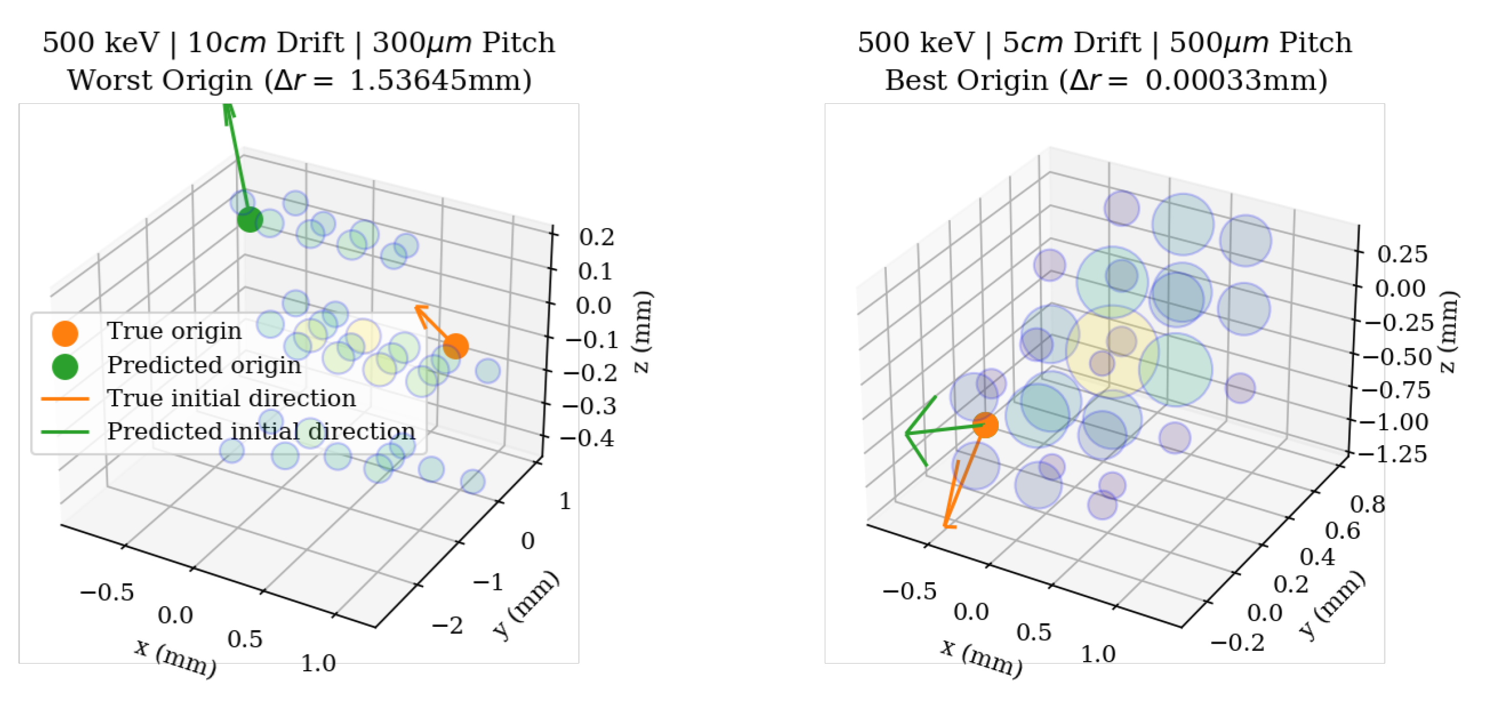
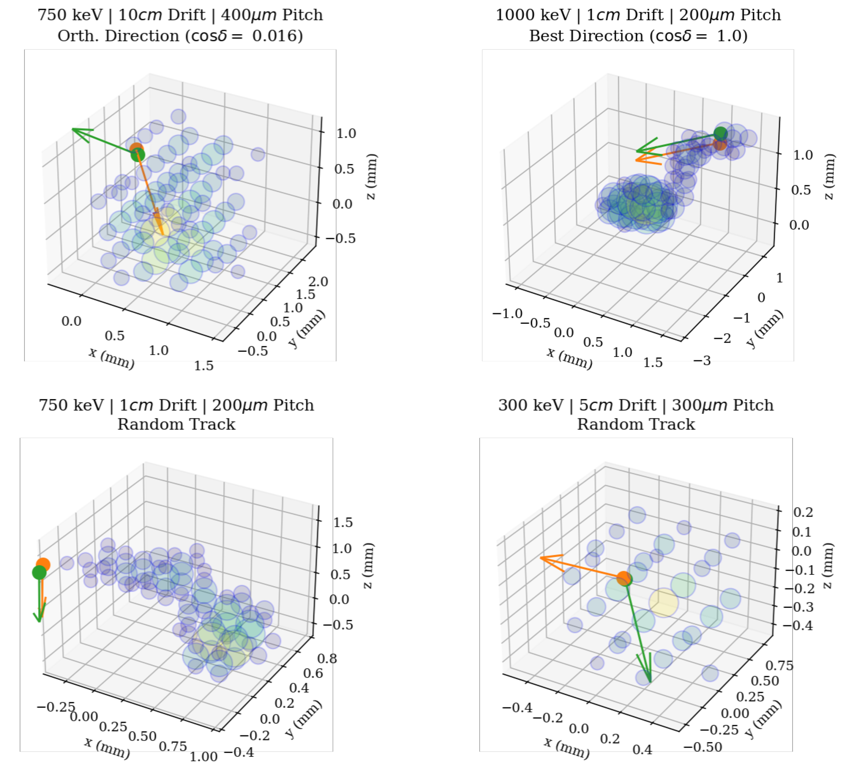
Section 4 and specifically detail the high accuracy of the initial direction and initial interaction location model predictions. We also include plots of the electron tracks overlaid with visualizations of the models’ predictions. Results for models trained on a broader data set are shown in Section 5, and we conclude and present paths for future work in Section 6.

2. Related Work

Prior efforts focusing on electron track reconstruction may be divided into two approaches: physics based estimation and data driven estimation. The reconstruction of general electron tracks is of seminal importance for the fields of Compton telescopes and X-ray polarimetry and has been investigated by researchers in both the disciplines.
With respect to physics based estimation, Bellazzini et al. [8] outlined the Momentum Method for reconstructing the direction of photo-electron emission. Recently, Li et al. [9] presented an algorithm based on graph theoretic concepts for X-ray polarimetry. Yoneda et al. [10] have attempted to apply this technique to electron-tracking Compton cameras. These techniques are inherently limited as they are applicable to strip based detectors only. In this context, Bernard et al. [11] have outlined the potential accuracy of time projection chambers for providing a photon direction measurement for Compton events, along with the polarimetry of linearly polarized radiation.
With respect to data driven estimation, there has been limited prior work carried out in this context, wherein Machine Learning algorithms have been applied for similar electron track reconstruction. Ikeda et al. [12] and Takada et al. [13] have utilized a Convolutional Neural Networks based on the VGG [14] and the U-Net [15] (The U-Net architecture consists of a contracting section, and an expansive section that also performs concatenations with the features from the contracting section. This leads to an architecture that resembles the alphabet “U”, leading to the nomenclature) architectures to predict the scattering positions and electron recoil directions from track images from PIC anode and cathode strips. Similarly, Peirson et al. [16], Peirson and Romani [17] and Peirson and Romani [18] utilized an ensemble of deterministic neural networks corresponding to the ResNet [19] architecture trained on Monte Carlo event simulations for the IXPE detector.
Our work focuses on inputs of 3-D images, as opposed to the aforementioned strip based detectors that generated conventional images with a singleton channel as inputs for the ML model. The complexity of the input leads to ensuing complexity of the problem. Furthermore, the proposed GammaTPC instrument is a liquid-based detector and thus is able to reconstruct electrons with energies of O (100 keV) and above. The aforementioned studies focused on electrons of O (1 keV). The higher energy leads to additional challenges in the ML task. Additionally, the higher dimensionality of the input (3-D images) obviates the adoption of established CNN architectures, as in the aforementioned prior works. We design our own model architecture, as is described in the following section.

3. Methods

The input to the CNN model is a 3D image of the voxelized charge readout from the detector. We simulate this readout in two steps. First, because GammaTPC is an instrument concept, real data is not yet available, so we use the PENetration and Energy LOss of Positrons and Electrons (PENELOPE) [20] code to simulate the energy loss along the tracks created by scattered electrons (A copy of PENELOPE can be obtained from the Nuclear Energy Agency at the following link: https://www.oecd-nea.org/tools/abstract/detail/nea-1525/, accessed on 1 November 2022). PENELOPE provides a detailed simulation of electron transport through various media (in this case, liquid argon), including elastic and inelastic scatters off of atoms, bremsstrahlung, and electron-positron pair production. The output is a table containing a series of steps through the medium, with each corresponding to one of the aforementioned interaction types. At each step, the energy deposited is recorded, as well as any daughter particles, which are also tracked. Chaining the steps together provides the simulated electron track. In the second step of our simulation pipeline, we use a custom code that simulates the creation of clouds of ionized electrons from the energy deposited along the electron track, the diffusion of these clouds as electrons drift to the pixel readouts, and the readout of the charge collected on the pixels. The drift distance of the charge to the detector, the readout noise, and pixel threshold are all adjustable parameters in this custom detector effects and readout code.
As the machine learning model acts as a surrogate for a physics phenomenon, it needs to mimic the underlying characteristics of the physical process. Based on physical criteria, the learning algorithm to approximate the mapping should have translational invariance and subsume locality in the mapping. The translational invariance is desired as the behavior of scattered electrons is independent of their position in the TPC, at least to the degree of analysis relevant for this work. Additionally, the locality would enable the model to consider voxels in spatial proximity to learn the head and direction. As convolutional layers are equivariant to spatial translations [21,22], they are a judicious choice for this task. When coupled with pooling layers, they are approximately translation invariant [21,22,23,24]. That is, convolution-based feature extraction is not affected by the absolute position of the feature in the feature map. Additionally, the convolution operation preserves locality of features conditioned upon the extent of the filter sizes [25]. Based on these criteria for the inductive biases of the learning algorithm, we utilize a convolutional neural network to learn a mapping from the raw three-dimensional images of the charge readout due to Compton scatters in the LArTPC to the location of the electron track head or the initial direction of the scattered electron.
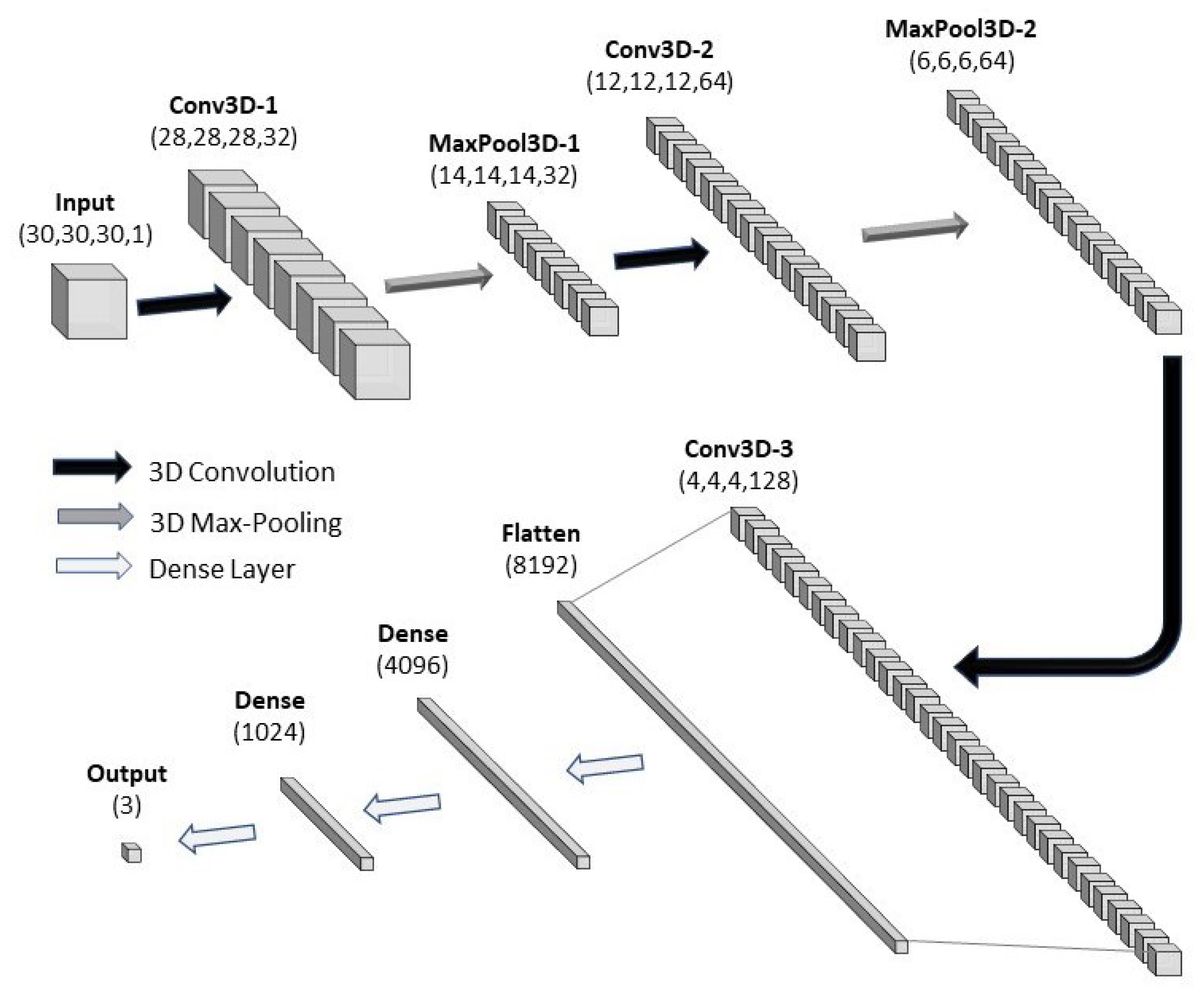
We include spatial dropout [26,27] and batch normalization [28] layers after each convolutional layer to reduce overfitting. The feature maps are flattened at the conclusion of the feature extraction stages that utilize three-dimensional convolutions. The final output from the fully connected layers is a 3-dimensional prediction for the location of the electron track head or of the initial direction of the scattered electron. The model architecture and ancillary hyperparameters were established based on Bayesian Optimization, followed by subsequent manual fine tuning. The outline of the model architecture utilized in this investigation is similar to Buuck et al. [29], where a probabilistic analysis of the the reconstruction was executed. Our head model uses an MSE loss function, though the initial direction model uses a cosine loss function, for the magnitude of the initial direction vector is not a quantity relevant to the kinematic reconstruction. Furthermore, we include a flatten layer for the head and initial direction models instead of a global average pooling layer as done in their work. A schematic of the model is shown in Figure 1.
The substitution of a global average pooling layer with a flatten layer increases the model complexity, though this is justified given the size of our data set compared to Buuck et al. [29]. Approximately 100,000 electron tracks were generated with PENELOPE for each of the chosen energies ranging from 50 to 1000 keV and were split in a 95:5 ratio for training/validation and testing; the same ratio was used for splitting the training and validation datasets. Individual models were trained on each of the energies with batch sizes of 64. We used the Adam optimizer with an initial learning rate of 10 3 and decreased this by a factor of four if no improvement was made to the validation loss after four consecutive epochs with 100 epochs in total. Furthermore, we halted training if the learning rate was below 10 8 and the validation loss did not decrease after 12 consecutive epochs. The typical training time for the direction and head models in Section 4 was 1.5 h and 30 min, respectively, while the models in Section 5 took approximately 7.5 h to train. Our training scripts are publically available (
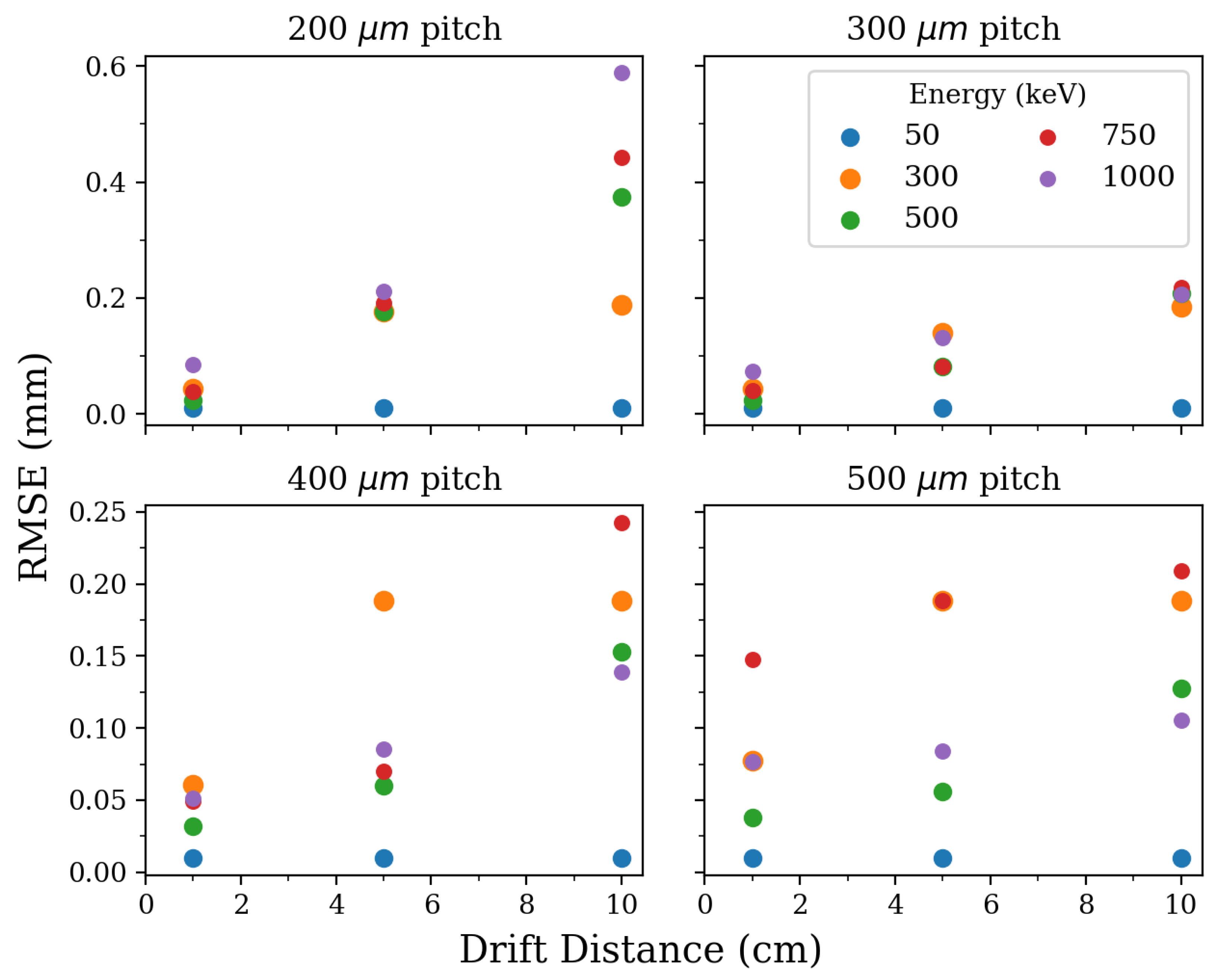
https://gitlab.com/gammatpc-ml/data-set-and-training-scripts, accessed on 1 November 2020), and additional code or data is available upon request. Finally, for our readout simulation, we use drift distances of 1, 5, and 10 cm for each energy and 200, 300, 400, and 500 μ m pixel pitches.

4. Model Results for Separated Energy and Drift Distance Data

In this section, we present the results for the head and initial direction models where we train a separate model for each energy and drift distance. Training the models on the data set in this manner allows for direct comparison to previous work [29] and highlights the advantage of the new model and additional data.

4.1. Track Origin Predictions

Figure 2 displays the error across all coordinates for various drift lengths. A bug in the code simulating the detector response caused some electrons to create tracks in the liquid argon with no detectable charge cloud, leading to populations of events with anomalously large Euclidean Distance Errors (greater than 5 mm). We have removed those events before generating Figure 2. All Aggregated Coordinate Error histograms, when fitted to normal distributions, have standard deviations different from each other with p-values smaller than 6.8 × 10 15 . Tracks corresponding to low energy events typically result in localized regions of charge sometimes less than 1 mm in extent, thus we can obtain small error for the track origin predictions. Higher energy electrons tend to have both longer and straighter tracks. Therefore, one might expect that it would be easier to correctly identify the beginning of a high energy electron track than a shorter, more circuitous low energy electron track. However, the smaller error for high energy tracks is not observed, and we speculate that the correlation between the typical error and track energy is present by virtue of the length scale of the track. Long tracks associated with high energies span distances on the order of a few mm, thereby allowing incorrect head predictions to produce errors larger than the incorrect predictions in tracks spanning sub-mm scales.
We also present a comparison of the error for the head models between the 1, 5, and 10 cm drift length data sets in Figure 3, which demonstrates that the scatters that happen at greater drift distances—that is, farther from where readout occurs—have worse position resolution. Because the charges have to drift farther, they also diffuse more, which worsens the definition of the charge cloud and washes out the shape of the electron track. We hypothesize that this is what causes the degradation in position resolution with increasing drift depth. Nonetheless, we find that the desired sub-mm accuracy is achievable for our model. The summary of our results for all pixel pitches can be found in Table 1.
We can make a comparison to the results achieved by Ikeda et al. [12], although there are some important differences between the experiments (chiefly their use of gaseous argon instead of liquid, their lower energy range, and the fact that their strip-based readout only produces two 2D images, compared to the full 3D readout achieved with GammaTPC). Ikeda et al. [12] show in their manuscript’s Figure 7a median absolute error on their position measurement between approximately 0.3 and 3.5 mm across their simulated energy range of 5 to 200 keV (right panel, red line). Comparatively, as shown in Figure 3, GammaTPC achieves an RMSE on our position measurement better than 0.2 mm in almost all cases across our simulated energy range of 50 to 1000 keV. Ikeda et al. [12] also show in their manuscripts’s Figure 7a median angular resolution between approximately 25 and 90° (left panel, red line). We obtain an angular resolution between 65 and 90° for 300 keV electrons, depending on depth, and between 1.6 and 2.2° for 1000 keV electrons, again depending on depth. Electrons with energies between 300 keV and 1000 keV have angular resolutions between these values, and at all energies the best resolution is obtained for short drift lengths, while the worst is for long drift lengths.

4.2. Initial Direction Predictions

In contrast to the origin predictions, it is easier to obtain smaller error for the initial direction of gamma photons with larger energies. Energetic electron recoil events result in longer tracks, therefore making the initial direction more well defined. This is exemplified in Figure 4, where our model demonstrates very strong predictive capability for higher energies and is conversely not performant for low energy scatters. The model is largely incapable of producing consistently correct predictions of the initial direction with 300 keV energies, therefore we omit the 50 keV events in the analysis here, for the model is expected to perform similarly or more poorly. We have performed a Cramer-von Mises test to determine the degree to which these distributions deviate from uniform distributions. All distributions shown in Figure 4 deviate from uniform distributions with p-values < 10 6 , with the exception of 300 keV electrons at 5 cm drift, which has a p-value of 9.58 × 10 5 and 300 keV electrons at 10 cm drift, which has a p-value of 0.86. The data in Figure 4 can also be summarized in Table 2, where we show the median of the error across all energies per drift distance and pixel pitch.
It is also interesting to evaluate the performance of the direction model when it is interpolating. Scattering events in the detector are not necessarily at the energies the models have been trained on, therefore we are required to create and train a model such that it maintains adequate predicting capability on a continuum of energies. Our results are shown in Figure 5. Here, we have taken the median of the errors across all tracks for each matrix element in the plot. The direction model maintains performance when tested on the energies it is trained on. However, it seems to have poor interpolation ability; it shows suboptimal performance even for scattering events with energies close to those it was trained on.

4.3. Visualization of Selected Electron Tracks

The charge the detector reads out and the models’ predictions of the origin and direction can be found in Figure 6 for selected electron tracks. It is important to note that the performance of the models is independent of one another despite the fact that the initial direction and interaction vertex are not. This is exemplified in the 750 keV/10 cm drift/400 μ m pitch track in which a highly accurate head prediction is achieved with a largely erroneous initial direction. Furthermore, we find that the model has difficulty finding the true initial direction for curled tracks as exemplified in the 300 keV/5 cm/300 μ m track. This aligns with intuition given the fact that the charge is too condensed to resolve the track and obtain a direction. On the contrary, we achieve low error in the origin prediction as a consequence of the tight track geometry.

5. Model Results for Aggregated Energy and Drift Distance Data

In GammaTPC, the energy of the incident photons and drift distances of the electrons will be variable. An effective head and initial direction model will therefore be able to maintain accuracy in stochastic conditions. We are then motivated to train a head and direction model across the three drift lengths and gamut of energies for each pixel pitch and compare the results to the models trained only on one energy and drift length. None of the hyperparameters used for the models in the previous section were changed here.

5.1. Track Origin Predictions

We have found that the head model trained across all energies and drift distances performs slightly worse than its energy- and drift- specific counterparts as shown in Figure 7 with median errors included in the caption. Sub-mm accuracy is still viable for 200 μ m and 400 μ m pitches, though we omit plots for the 300 μ m and 500 μ m pitches because these models failed to train. The standardized hyperparameters used throughout this investigation resulted in minimal reduction of the validation loss for the the 300 μ m and 500 μ m pitch models during training, rendering their predictions unchanged by the input. Although the correlation between error and energy is not as consistent as with the head models in Section 4, the overall trend observed here can be explained by the same physical reasoning. The fact that the 750 keV tracks have less accurate predictions than the 1000 keV tracks do not have an obvious physical interpretation, but could instead be artifacts of the model training and hyperparameters. The model has not been fine tuned for each pitch or drift distance, and this limitation manifests in the form of accuracies that differ from those in the preceding section.

5.2. Initial Direction Predictions

Accuracy for the models trained across all energies and drift distances are shown in Figure 8. Commonalities with previous models include an improvement in performance from the 200 μ m to 300 μ m pitch as seen previously Figure 3, as well as prediction errors being relatively similar for the direction models as seen before in Figure 4.
Nonetheless, the models are slightly less performant compared to those discussed in Section 4. It is possible that a more complex model is needed to take full advantage of the approximately 1.2 million electron tracks that were available for training. Nonetheless, the models are still able to consistently deliver reasonably precise estimates, especially at small drift distances and high energies where we can reliably achieve predictions with errors smaller than 10°.
The model is evaluated at energies beyond those present in the trained data set, and the results are displayed in Figure 9 with the vertical axis showing the median of the error cos δ across all of the test tracks for a particular energy. The relatively better performance for the trained energies 300, 500, 750 and 1000 keV is expected. While the interpolation ability of the model is expected to have improved compared to the models in Section 4 due to the broader training data set, we still find no correlation between the prediction error and the energy difference from an energy used in training. That is, scattering events with energy levels outside those the model has been trained on, regardless of the energy difference from a trained energy, yield similar errors.

6. Conclusions and Future Work

We have developed machine learning models to predict the origin and initial direction of the electron recoil events in the proposed liquid argon gamma ray observatory GammaTPC. The precision of the reconstruction of the electron tracks is a major driver in the overall ability of the instrument to locate gamma ray sources on the sky. Consequently, the optimized pointing capability of GammaTPC gives rise to strong discovery potential for phenomena associated with gamma ray emission in the low MeV range, allowing for deeper insight on phenomena ranging from black hole jets to WIMP dark matter.
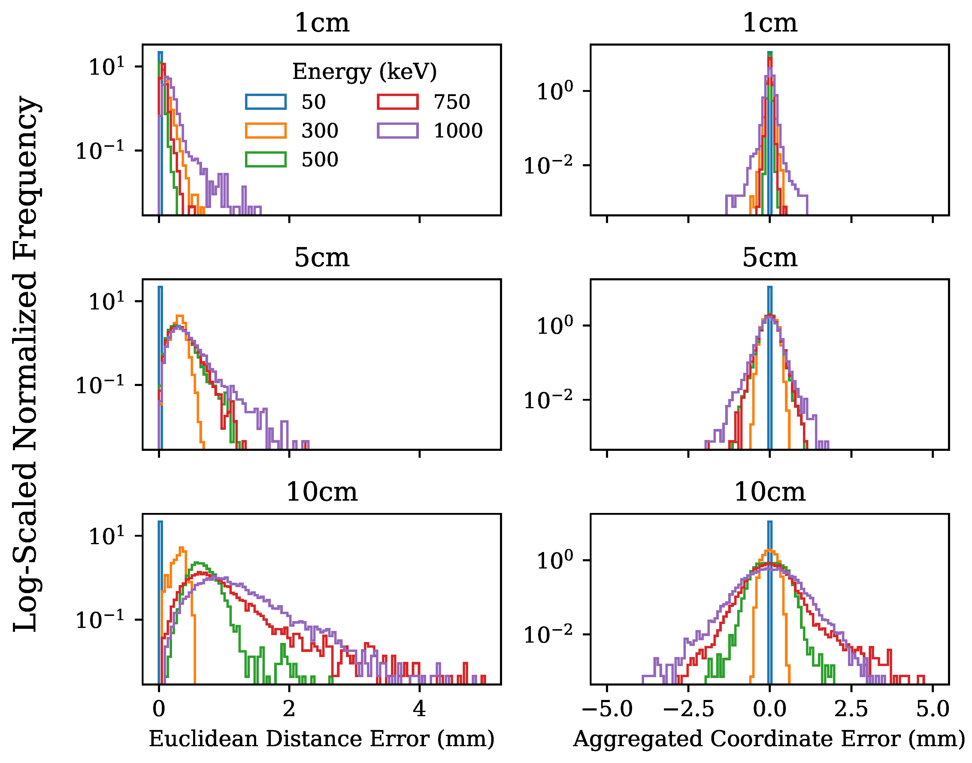
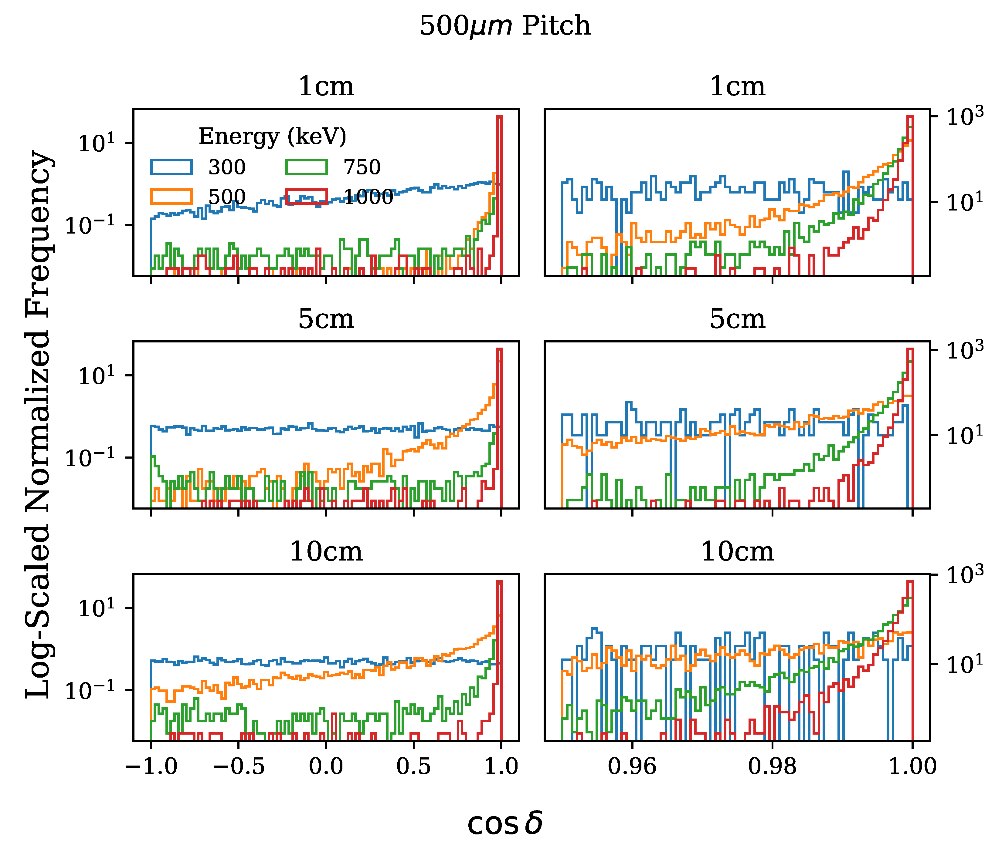
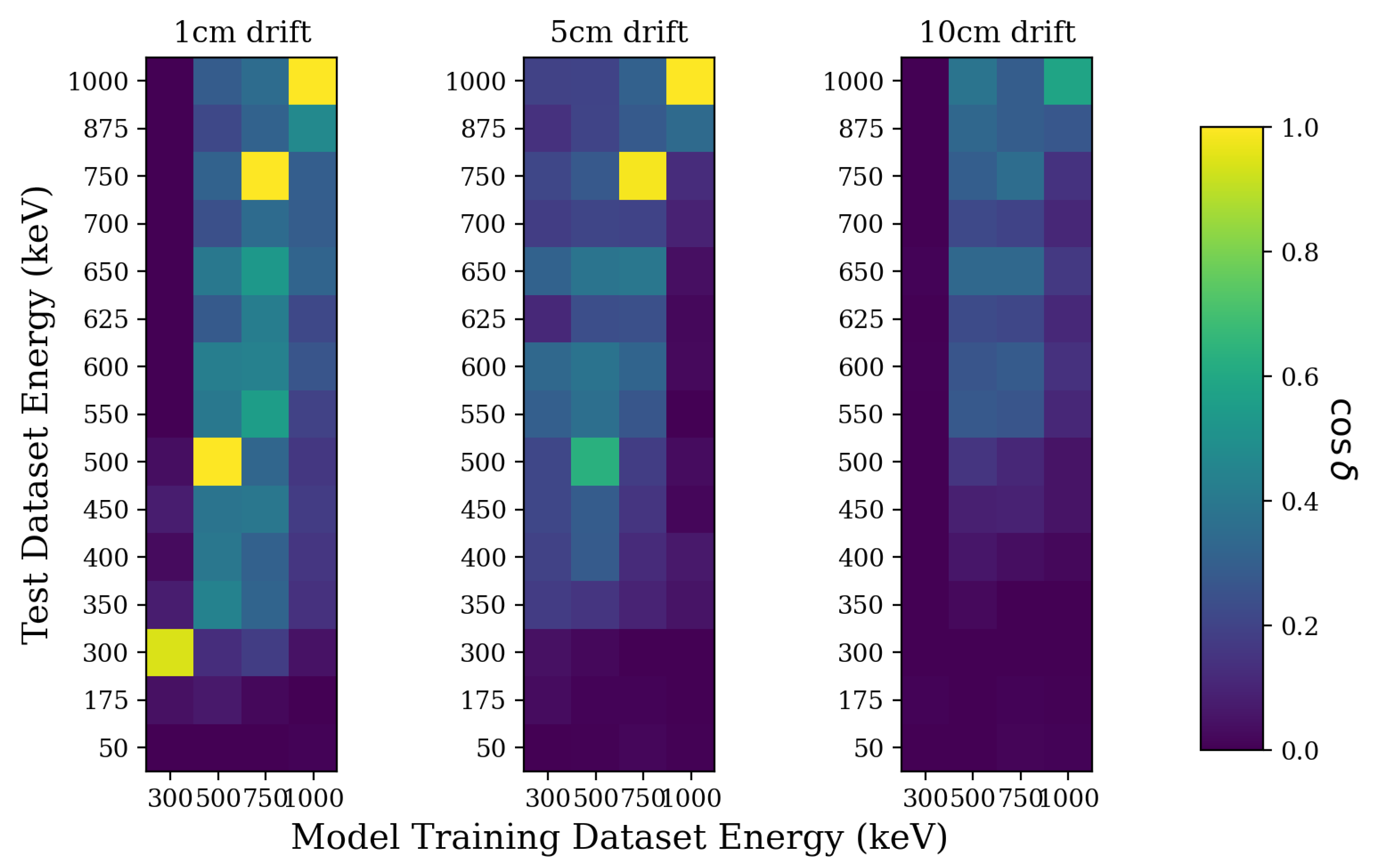
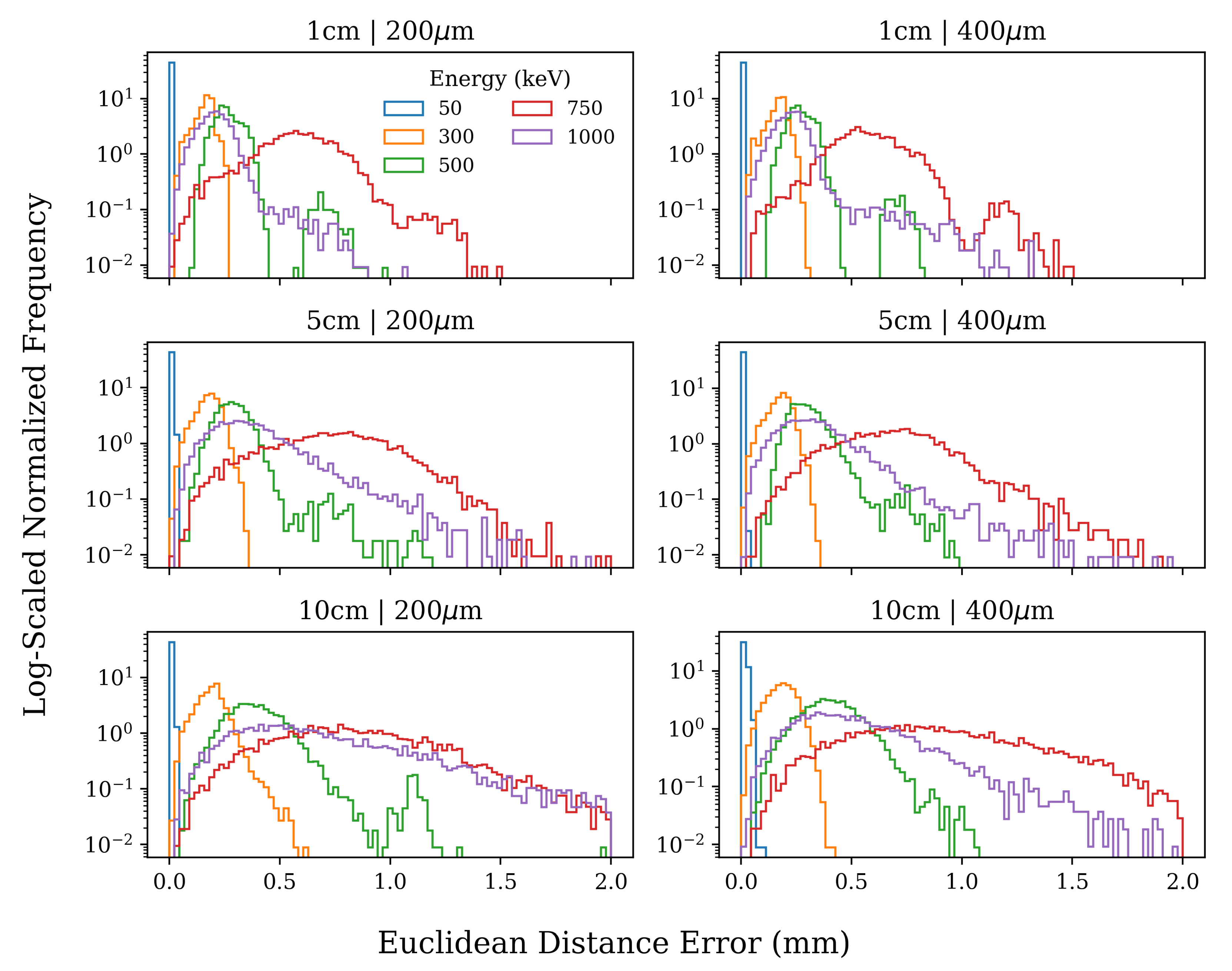
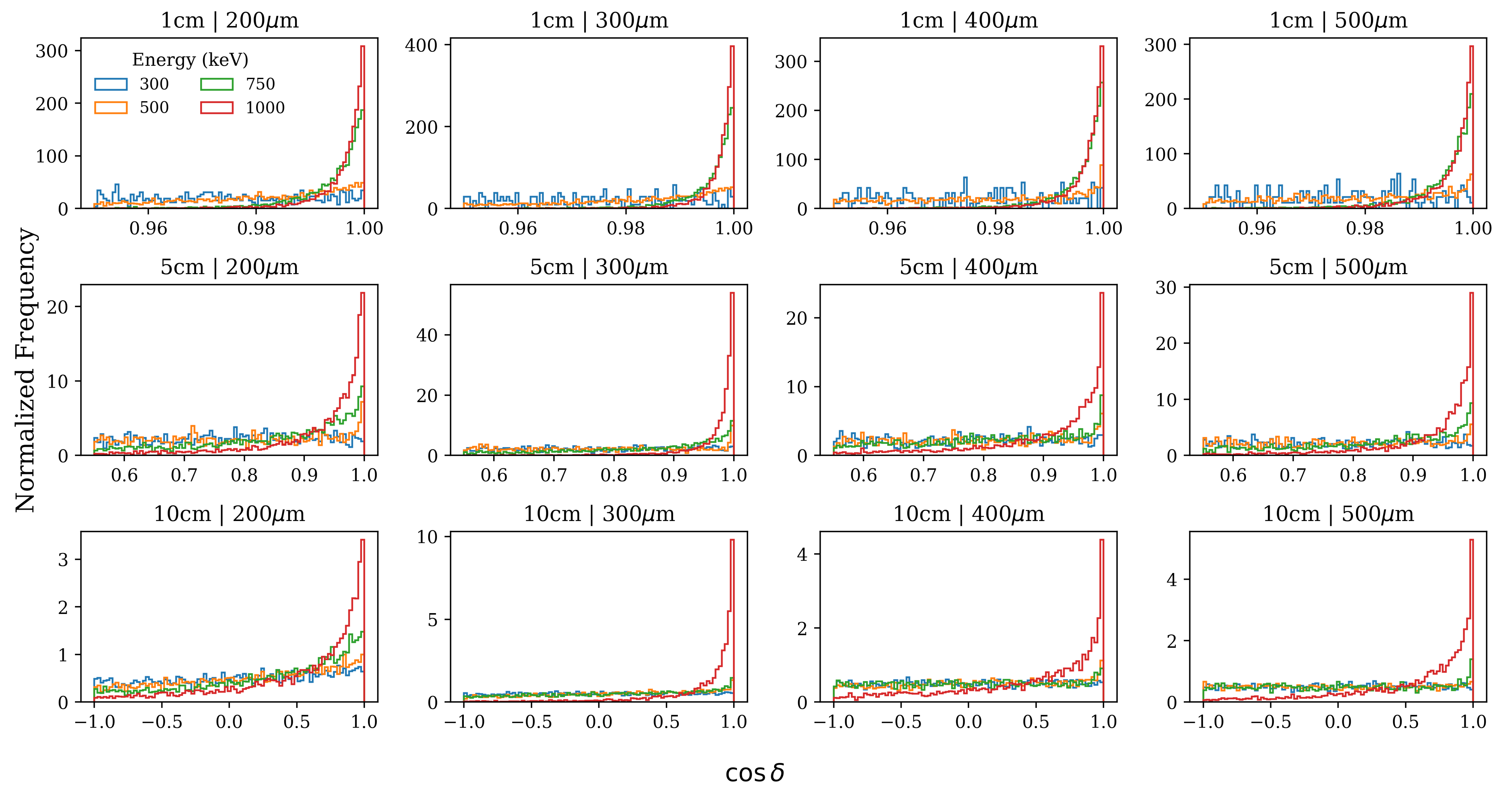
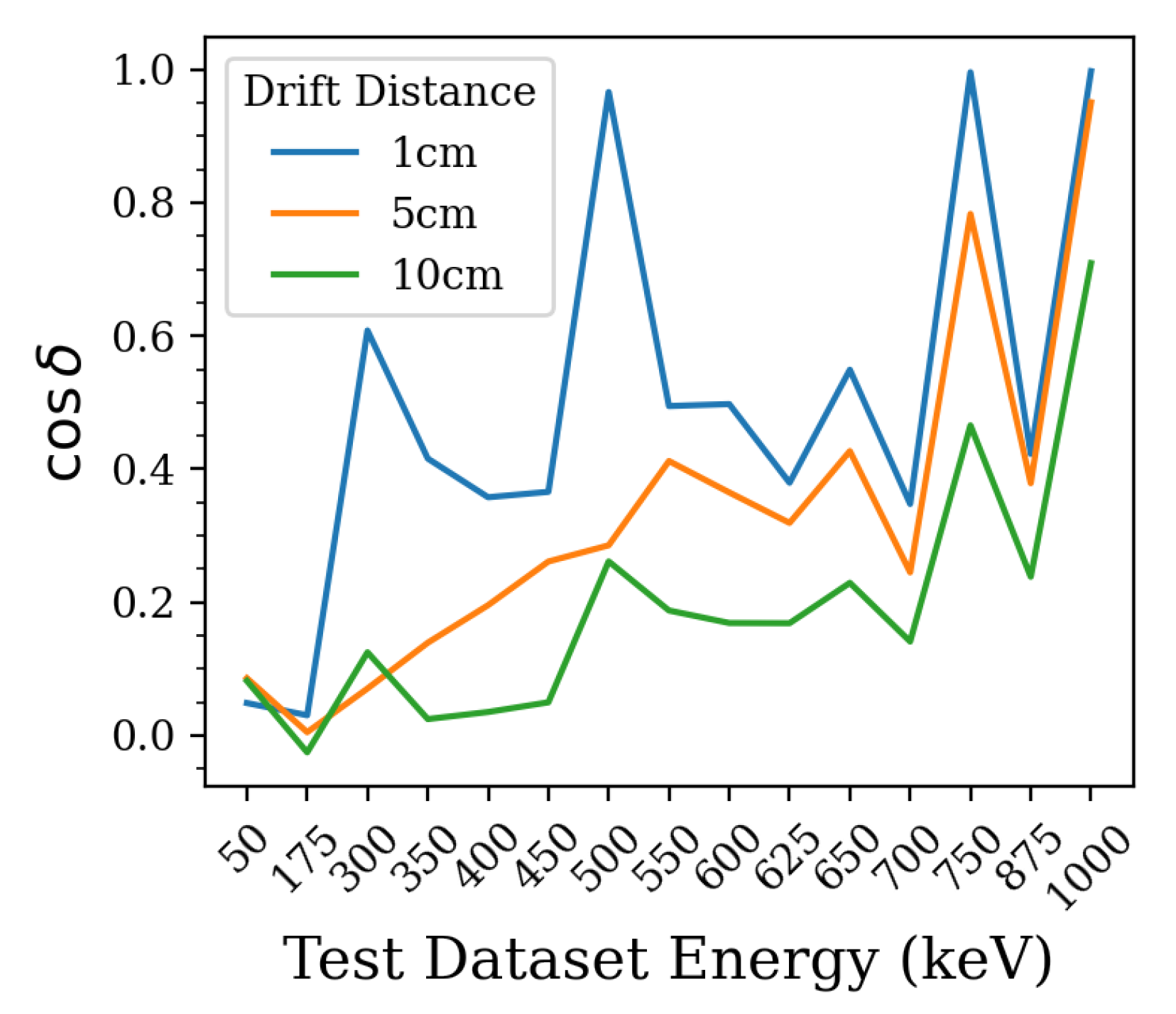
We have found that sub-mm accuracy for the track origin predictions is possible for the low energy events, especially at small drift lengths. Our initial direction model predicts the initial direction exceptionally for high energy events. At energies of 500 keV and below, the direction model is significantly less accurate, and at long drift distances it is largely incapable of determining the initial direction. We have tested the limits of the head and initial direction models by training them over a spectrum of energies and drift distances, finding that the larger dataset mitigates the models’ efficacies. The broadly trained models are less performant for energies that they are trained on compared to the specialized models, and they have little ability to interpolate to make predictions on events with energies not in the training data set.
It is possible to localize gamma ray sources more precisely by quantifying the uncertainty with the estimates from the machine learning models, and we intend to explore this with post-hoc methods such as the Laplace Approximation [30] in future work. As it stands, the models only provide point predictions of the initial direction and head location. Quantifying the uncertainty allows us to remove erroneous predictions that don’t contribute to the source localization. We also look forward to tuning the model hyperparameters so that it maintains adequate predicting capability when training data consists of mixed energies and drift lengths.

Author Contributions

Conceptualization, B.K. and A.M.; methodology, B.K., M.B. and A.M.; software, B.K. and A.M.; validation, B.K. and A.M.; formal analysis, B.K. and A.M.; investigation, B.K., M.B. and A.M.; resources, B.K. and A.M.; data curation, B.K., M.B. and A.M.; writing—original draft preparation, B.K., M.B. and A.M.; writing—review and editing, B.K., M.B., T.S. and A.M.; visualization, B.K., M.B. and A.M.; supervision, B.K., M.B. and A.M.; project administration, B.K., M.B. and A.M.; funding acquisition, B.K., M.B., T.S. and A.M. All authors have read and agreed to the published version of the manuscript.

Funding

This research was supported by the U.S. Department of Energy and SLAC National Accelerator Laboratory. This work was also supported in part by funding from Zoox Inc.

Institutional Review Board Statement

Not applicable.

Informed Consent Statement

Not applicable.

Data Availability Statement

The data used in this study will be made available upon reasonable request.

Acknowledgments

This research was supported by the U.S. Department of Energy and SLAC National Accelerator Laboratory.

Conflicts of Interest

The authors declare no conflict of interest. The funders had no role in the design of the study; in the collection, analyses, or interpretation of data; in the writing of the manuscript; or in the decision to publish the results.

Abbreviations

The following abbreviations are used in this manuscript:
LArLiquid Argon
TPCTime Projection Chamber
WIMPWeakly Interacting Massive Particle
COMPTELCompton Telescope
OSSEOriented Scintillation Spectrometer Experiment
CNNConvolutional Neural Network
MLMachine Learning
MSEMean Squared Error
VGGVisual Geometry Group
PICPixel Chamber
ResNetResidual Neural Network

References

  1. McEnery, J.; Barrio, J.A.; Agudo, I.; Ajello, M.; Álvarez, J.; Ansoldi, S.; Anton, S.; Auricchio, N.; Stephen, J.B.; Baldini, L.; et al. All-sky Medium Energy Gamma-ray Observatory: Exploring the Extreme Multimessenger Universe. arXiv 2019, arXiv:1907.07558. [Google Scholar]
  2. Cembranos, J.A.; Strigari, L.E. Diffuse MeV gamma rays and galactic 511 keV line from decaying WIMP dark matter. Phys. Rev. D 2008, 77, 123519. [Google Scholar] [CrossRef] [Green Version]
  3. Lawson, K.; Zhitnitsky, A.R. Diffuse cosmic gamma rays at 1–20 MeV: A trace of the dark matter? J. Cosmol. Astropart. Phys. 2008, 2008, 022. [Google Scholar] [CrossRef]
  4. Tomsick, J.; Zoglauer, A.; Sleator, C.; Lazar, H.; Beechert, J.; Boggs, S.; Roberts, J.; Siegert, T.; Lowell, A.; Wulf, E.; et al. The compton spectrometer and imager. Bull. Am. Astron. Soc. 2019, 51, 98. [Google Scholar]
  5. Shutt, T. Development of a Novel Readout System for a Liquid Argon Time Projection Chamber MeV Gamma-Ray Telescope. In Proceedings of the SnowMass 2021 Meeting, Seattle, WA, USA, 4 November 2021. [Google Scholar]
  6. Aramaki, T.; Boezio, M.; Buckley, J.; Bulbul, E.; von Doetinchem, P.; Donato, F.; Harding, J.P.; Karwin, C.; Kumar, J.; Leane, R.K.; et al. Snowmass2021 Cosmic Frontier: The landscape of cosmic-ray and high-energy photon probes of particle dark matter. arXiv 2022, arXiv:2203.06894. [Google Scholar]
  7. Cooper, M.; Mijnarends, P.; Shiotani, N.; Sakai, N.; Bansil, A. X-ray Compton Scattering; OXford University Press: Oxford, UK, 2004; Volume 5. [Google Scholar]
  8. Bellazzini, R.; Angelini, F.; Baldini, L.; Brez, A.; Costa, E.; Di Persio, G.; Latronico, L.; Massai, M.M.; Omodei, N.; Pacciani, L.; et al. Novel gaseous X-ray polarimeter: Data analysis and simulation. In Proceedings of the Astronomical Telescopes and Instrumentation, Waikoloa, HI, USA, 22–28 August 2002; Volume 4843, pp. 383–393. [Google Scholar]
  9. Li, T.; Zeng, M.; Feng, H.; Cang, J.; Li, H.; Zhang, H.; Zeng, Z.; Cheng, J.; Ma, H.; Liu, Y. Electron track reconstruction and improved modulation for photoelectric X-ray polarimetry. Nucl. Instrum. Methods Phys. Res. Sect. A Accel. Spectr. Detect. Assoc. Equip. 2017, 858, 62–68. [Google Scholar] [CrossRef] [Green Version]
  10. Yoneda, H.; Saito, S.; Watanabe, S.; Ikeda, H.; Takahashi, T. Development of Si-CMOS hybrid detectors towards electron tracking based Compton imaging in semiconductor detectors. Nucl. Instrum. Methods Phys. Res. Sect. A Accel. Spectr. Detect. Assoc. Equip. 2018, 912, 269–273. [Google Scholar] [CrossRef] [Green Version]
  11. Bernard, D.; Hunter, S.D.; Tanimori, T. Time projection chambers for gamma-ray astronomy. arXiv 2022, arXiv:2206.08676. [Google Scholar]
  12. Ikeda, T.; Takada, A.; Abe, M.; Yoshikawa, K.; Tsuda, M.; Ogio, S.; Sonoda, S.; Mizumura, Y.; Yoshida, Y.; Tanimori, T. Development of convolutional neural networks for an electron-tracking Compton camera. Prog. Theor. Exp. Phys. 2021, 2021, 083F01. [Google Scholar] [CrossRef]
  13. Takada, A.; Takemura, T.; Yoshikawa, K.; Mizumura, Y.; Ikeda, T.; Nakamura, Y.; Onozaka, K.; Abe, M.; Hamaguchi, K.; Kubo, H.; et al. First Observation of the MeV Gamma-Ray Universe with Bijective Imaging Spectroscopy Using the Electron-tracking Compton Telescope on Board SMILE-2+. Astrophys. J. 2022, 930, 6. [Google Scholar] [CrossRef]
  14. Simonyan, K.; Zisserman, A. Very deep convolutional networks for large-scale image recognition. arXiv 2014, arXiv:1409.1556. [Google Scholar]
  15. Ronneberger, O.; Fischer, P.; Brox, T. U-net: Convolutional networks for biomedical image segmentation. arXiv 2015, arXiv:1505.04597. [Google Scholar]
  16. Peirson, A.; Romani, R.; Marshall, H.; Steiner, J.; Baldini, L. Deep ensemble analysis for Imaging X-ray Polarimetry. Nucl. Instrum. Methods Phys. Res. Sect. A Accel. Spectr. Detect. Assoc. Equip. 2021, 986, 164740. [Google Scholar] [CrossRef]
  17. Peirson, A.; Romani, R. A deep ensemble approach to X-ray polarimetry. arXiv 2021, arXiv:2111.03047. [Google Scholar]
  18. Peirson, A.; Romani, R.W. Toward optimal signal extraction for imaging x-ray polarimetry. Astrophys. J. 2021, 920, 40. [Google Scholar] [CrossRef]
  19. He, K.; Zhang, X.; Ren, S.; Sun, J. Deep residual learning for image recognition. In Proceedings of the IEEE Conference on Computer Vision and Pattern Recognition, Las Vegas, NV, USA, 27–30 June 2016; pp. 770–778. [Google Scholar]
  20. Agency, N.E. PENELOPE 2018: A Code System for Monte Carlo Simulation of Electron and Photon Transport; Nuclear Energy Agency: Paris, France, 2019; p. 420. [Google Scholar] [CrossRef] [Green Version]
  21. Bronstein, M.M.; Bruna, J.; Cohen, T.; Veličković, P. Geometric deep learning: Grids, groups, graphs, geodesics, and gauges. arXiv 2021, arXiv:2104.13478. [Google Scholar]
  22. Karniadakis, G.E.; Kevrekidis, I.G.; Lu, L.; Perdikaris, P.; Wang, S.; Yang, L. Physics-informed machine learning. Nat. Rev. Phys. 2021, 3, 422–440. [Google Scholar] [CrossRef]
  23. Kauderer-Abrams, E. Quantifying translation-invariance in convolutional neural networks. arXiv 2017, arXiv:1801.01450. [Google Scholar]
  24. Ihme, M.; Chung, W.T.; Mishra, A.A. Combustion machine learning: Principles, progress and prospects. Prog. Energy Combust. Sci. 2022, 91, 101010. [Google Scholar]
  25. Goodfellow, I.; Bengio, Y.; Courville, A. Deep Learning; MIT Press: Cambridge, MA, USA, 2016. [Google Scholar]
  26. Tompson, J.; Goroshin, R.; Jain, A.; LeCun, Y.; Bregler, C. Efficient object localization using convolutional networks. In Proceedings of the IEEE Conference on Computer Vision and Pattern Recognition, Boston, MA, USA, 7–12 June 2015; pp. 648–656. [Google Scholar]
  27. Srivastava, N.; Hinton, G.; Krizhevsky, A.; Sutskever, I.; Salakhutdinov, R. Dropout: A simple way to prevent neural networks from overfitting. J. Mach. Learn. Res. 2014, 15, 1929–1958. [Google Scholar]
  28. Ioffe, S.; Szegedy, C. Batch normalization: Accelerating deep network training by reducing internal covariate shift. In Proceedings of the International Conference on Machine Learning, Lille, France, 6–11 July 2015; pp. 448–456. [Google Scholar]
  29. Buuck, M.; Mishra, A.; Charles, E.; Di Lalla, N.; Hitchcock, O.; Monzani, M.E.; Omodei, N.; Shutt, T. Low-Energy Electron-Track Imaging for a Liquid Argon Time-Projection-Chamber Telescope Concept using Probabilistic Deep Learning. arXiv 2022, arXiv:2207.07805. [Google Scholar]
  30. Daxberger, E.; Kristiadi, A.; Immer, A.; Eschenhagen, R.; Bauer, M.; Hennig, P. Laplace redux-effortless bayesian deep learning. Adv. Neural Inf. Process. Syst. 2021, 34, 20089–20103. [Google Scholar]
Figure 1. Diagram of the model architecture used in our investigation. A cosine loss function was used for the initial direction model and MSE loss for the head model.
Ai 03 00058 g001
Figure 2. Accuracy of the head model for the 200 μ m pixel pitch case. Left column: Euclidean distance between the true and predicted head locations. Right column: Difference between the true and predicted head coordinate aggregated across all coordinate directions.
Ai 03 00058 g002
Figure 3. Comparison of the head model predicting accuracy by energy per drift length. Longer drift lengths result in origins that are harder to predict due to the diffusion of charge, and hence loss of information, before readout. Points sizes differ in order to reveal overlapping points.
Ai 03 00058 g003
Figure 4. Comparison of the direction model predicting accuracy by energy per drift length for the 500 μ m pitch case. Left column: Cosine of the angle between the true and predicted initial electron recoil directions for the initial direction model at drift lengths 1, 5, and 10 cm. Right column: Magnified view of the left column.
Ai 03 00058 g004
Figure 5. Error for models trained on one energy and drift length and tested on energies from both the data set and outside it. Each pixel in the grid is the median of the error cos δ for the 5000 tracks in the test data set.
Ai 03 00058 g005
Figure 6. Selected 3D plots of the electron tracks at various energies, drift distances, and pixel pitches. The color and size of the circles indicates the amount of charge read out at a particular voxel. We denote Δ r as the euclidean distance between the predicted and target origins, and cos δ as the cosine of the angle between the predicted and target initial direction vectors.
Ai 03 00058 g006aAi 03 00058 g006b
Figure 7. Euclidean distance error for the head models trained on data composed of all energies and drift distances at a particular pitch. The median after combining all energy distributions in the 200 μ m column is 0.20114, 0.24877 and 0.33071 mm for the 1, 5 and 10 cm drift distances, respectively. Likewise, the 400 μ m column gives median errors of 0.21661, 0.24439, and 0.31654 mm.
Ai 03 00058 g007
Figure 8. Prediction error for direction models trained over all energies and drift distances for a fixed pixel pitch where δ is the the angle between predicted and true initial electron direction. Combining all energies at a fixed drift length, the median δ is approximately the same across all pixel pitches and is around 10, 50 and 70 degrees for the 1, 5, and 10 cm drift distances.
Ai 03 00058 g008
Figure 9. Error for initial direction models trained on the 200 μ m pitch data across energies 300, 500, 750, and 1000 keV and drift lengths 1, 5, and 10 cm. Models are tested on energies present in both the training data set (300, 500, 750, 1000 keV) and outside it. We only plot the median of the cosine of the error cos δ from the 5000 test tracks; larger cos δ implies more accurate predictions.
Ai 03 00058 g009
Table 1. Median Euclidean distance error (mm) for the head model across all energies, fixing one of the four pixel pitches and three drift distances.
Pixel Pitch ( μ m)
200300400500
Drift Distance (cm)10.056640.056210.066260.10167
50.281130.151460.121090.15662
100.516670.303430.260070.22308
Table 2. Median of the angle (in degrees) between the predicted and true initial direction vectors for various pixel pitches and drift lengths. Perfect predictions yield δ = 0 °.
Pixel Pitch ( μ m)
200300400500
Drift Distance (cm)12.03362.04433.0673.572
524.6607.43375.02455.3518
1072.97829.07817.20611.117
Publisher’s Note: MDPI stays neutral with regard to jurisdictional claims in published maps and institutional affiliations.

