Article

Vehicle State Estimation and Prediction for Autonomous Driving in a Round Intersection

Automated Driving Lab, Ohio State University, Columbus, OH 43210, USA
*
Author to whom correspondence should be addressed.
Vehicles 2023, 5(4), 1328-1352; https://doi.org/10.3390/vehicles5040073
Submission received: 4 July 2023 / Revised: 11 September 2023 / Accepted: 2 October 2023 / Published: 5 October 2023
(This article belongs to the Special Issue Path Tracking for Automated Driving)

Abstract

:
This paper presents methods for vehicle state estimation and prediction for autonomous driving. A round intersection is chosen for application of the methods and to illustrate the results as autonomous vehicles have difficulty in handling round intersections. State estimation based on the unscented Kalman filter (UKF) is presented in the paper and then applied to state estimation of vehicles in a round intersection. The microscopic traffic simulator SUMO (Simulation of Urban Mobility) is used to generate realistic traffic in the round intersection for the simulation experiments. Change point detection-based driving behavior prediction using a multipolicy approach is then introduced and evaluated for the round intersection. Finally, these methods are combined for vehicle trajectory estimation based on UKF and policy prediction and demonstrated using the round intersection.

1. Introduction

Connected and autonomous driving [1] including self-driving robot-taxis are becoming more widely available each year. A survey of autonomous driving common practices has been provided in [2]. Motion planning and motion planning and control methods for autonomous driving are reviewed in references [3,4,5], respectively. Reference [6] treats maneuver-based trajectory planning for highly automated vehicles on real roads. A survey of deep learning application for autonomous driving are provided in reference [7]. Reference [8] considers automated driving in uncertain environments, while reference [9] focuses on human-like empirical decision making for autonomous vehicles. Reference [10] focuses on the real-time nature of their motion planning for autonomous driving in urban environments. The autonomous driving systems, their feedback control loops, and decision-making systems in the above-cited references depend on the effectiveness of information collection and the knowledge of vehicle motions, including the ego vehicle and other nearby vehicles. Knowing this information, autonomous vehicles can estimate the behaviors and future positions of others so as to determine the correct way of behaving in their current traffic scenario. Therefore, the knowledge of the ego and nearby vehicle states at the current moment and being able to accurately predict their future motion and states is very important for safe autonomous driving.
The sensor suite commonly used in on-road autonomous vehicles includes GPS (Global Positioning System), IMU (Inertial Measurement Unit), lidar(s), camera(s), and radar(s). With the information collected from GPS and IMU, the ego vehicle can measure its state, including its global position, its heading angle for orientation, its linear velocity, its angular velocity, and its acceleration. With the information collected from these on-board sensors, current states and future state trajectories can be computed and estimated for the ego vehicle. However, the case is a lot different for other vehicles as compared to the ego vehicle. The task for estimating true object states and predicting future trajectories of other road users can become a difficult task due to the following reasons. First, perception sensors such as lidar, camera, and radar can provide positioning information and velocity information, but unlike the ego vehicle with onboard IMU, angular velocity and accelerations are hard to derive simply based on observations from these sensors. Additionally, sensor-based detections in autonomous vehicles are not exact. The data collection about other road users and objects are noisy measurements, which leads to errors in sensor detection and perception. Furthermore, not all the states of the other vehicles are observed or measured. Hence, the knowledge of motion of other road users is uncertain, especially in the urban traffic scenario. Unlike highway traffic, the acceleration, velocity, and heading angles can change suddenly due to complex traffic situations in urban driving environments. Road users need to be alerted promptly when an unexpected situation possibly takes place in the urban scenario, and this is even more severe when the traffic density is high. Hence, for the planning of autonomous driving, it is important to have good estimation and prediction of other road users so that the planning and control of the ego vehicle can be more efficient and robust towards the desired control objective.
Vehicle estimation and future state prediction have long been research problems of focus and a variety of solutions have been proposed. Estimation can be used for different types of nearby vehicle future behavior and information, especially for their states that are not directly measured, such as angular velocity and lateral velocity. Here, we call them the internal states. Several methods have been proposed for deriving the internal states from the measured vehicle trajectory. In [11], by assuming the ideal condition where vehicle tires have only pure rolling contact, the authors computed lateral velocity from longitudinal velocity and steering angle based on the single-track model or the so-called bicycle model. In [12], the authors compared different motion models for vehicle tracking and applied Kalman filtering for generating an estimated trajectory to illustrate the accuracy of motion models in describing vehicle motion while getting rid of sensor noise. Reference [12] provides a good reference for selecting the right motion model to describe vehicle motions under different road conditions. In [13], Real Time Kinematic (RTK)-based GPS correlation is applied for vehicle position information collected for estimating vehicle internal states which increase the precision of the collected information. More and more RTK-based GPS units are used for vehicles to improve the accuracy of their positioning system, which also benefits the vehicle state estimation.
With the fast development of artificial intelligence and neural network methods, image-based trajectory prediction also draws a lot of attention. In [14], a graph Long Short-Term Memory (graph-LSTM)-based trajectory prediction method is proposed by utilizing a series of images and representing the proximity between road agents using a weighted dynamic geometric graph. In [15], a spatio-temporal graph convolution neural network is proposed for predicting human trajectory on the road for vulnerable road user safety. There are also other neural network (NN)-based prediction methods utilizing LSTM or Recurrent Neural Networks (RNN) for the purpose of processing time series and predicting future such as [16].
In this paper, vehicle internal state estimation and vehicle policy prediction methods are introduced for predicting the future state and trajectories for other vehicles in the urban traffic scenarios, especially in the traffic scenario of round intersections. Kalman filter-based state estimation and change point detection-based policy prediction are introduced. A combined method for vehicle trajectory prediction is also proposed for better estimating the vehicle trajectory in a future time period, which will assist the decision making of the ego vehicle in the round intersection. Without loss of generality, we assume that the other road users that the ego vehicle encounter are vehicles. Vulnerable road users such as bicyclists and pedestrians are not considered in this paper.
The contributions of this paper are as follows. This paper presents a Bayesian change point detection-based policy prediction method. An existing change point detection method is modified here by introducing Kalman filter-based state estimation for generating a clean vehicle trajectory history for assisting the behavior prediction. A new method for solving the computation of the likelihood value for different vehicle policies for round intersections is introduced. This modified method also predicts the future dynamic behavior of the observed vehicle using the vehicle hidden states estimated by the Kalman filter. Behavior prediction is combined with the vehicle motion model for predicting vehicle behavior in the near future so that the estimated trajectory derived from the prediction method can assist in decision making.
The rest of the paper is organized as follows. State estimation based on the unscented Kalman filter is introduced with application to a round intersection in Section 2. The microscopic traffic simulator SUMO is used to generate realistic traffic in the round intersection for the simulation experiments of Section 2. Change point detection-based driving behavior prediction using a multipolicy approach is introduced in Section 3 and evaluated for the round intersection example. Section 4 combines the methods of Section 2 and Section 3 for vehicle trajectory estimation based on UKF and policy prediction. The paper ends with the usual conclusions in the last section.

2. State Estimation Based on Kalman Filter

The future motion and states of the ego vehicle can be predicted with on-board sensors such as GPS and IMU that provide information on position and motion, including velocity, acceleration, and angular velocity. However, for the case where we do not have any information or measurement on the vehicle motion, it is important to have a tool for calculating and estimating the internal states, which our sensors do not have access to. Kalman filter, the famous estimation algorithm, is a powerful and commonly used tool in those cases. The core idea of the Kalman filter and its central operation is the propagation of the Gaussian random variable through the system dynamic model [17]. An original Kalman filter can be used for solving the problem where the system dynamic equations are linear. However, the vehicle models are nonlinear, so the original Kalman filter is not applicable to solve the trajectory tracking and motion estimation problem. For the nonlinear case, several variations of the Kalman filter have been proposed. These include the extended Kalman filter (EKF) [18] and the unscented Kalman filter (UKF) [19]. The EKF approximates the states using Gaussian random variables by introducing the first-order linearization of the system dynamic of the nonlinear system. The UKF deals with the nonlinearity by representing the state distribution with sampling points, called sigma points, that capture true mean and covariance of the Gaussian random variables that describe the states and propagation through the nonlinear function without linearization. Both variations of the Kalman filter work well for the nonlinear case. However, the EKF, as discussed in [19], has some disadvantages. The first-order linearization of the system can introduce large errors for the posterior mean and covariance when the Gaussian random variables are propagated through the linearized state equation. Other than this error caused by linearization, the estimation based on EKF may also have sub-optimal performance, and sometimes will not converge. However, in the UKF, the propagation through dynamic equations of the sample points will not involve additional errors. The posterior mean and covariance will still be captured by the unscented transformation in the UKF. Hence, it outperforms the EKF and is implemented in this paper for estimating the vehicle internal states based on the observable measurements and collected data.

2.1. The Unscented Kalman Filter

The unscented Kalman filter is a variation of the Kalman filter based on the unscented transform (UT) that operates on the sampled sigma points that are used for representing the true mean and covariance of the state representation of Gaussian random variables. Consider a discrete nonlinear dynamical system expressed as follows:
x k + 1 = F ( x k , v k )
y k = H ( x k , n k )
where x k represents the states of the system at current time instant k. This system could be observable, partially observable, or hidden to the external observer and measurement. v k is the process noise that drives the system or disturbs the state transition of the whole system. y k is the current measurement that the external observer can access, and n k is the measurement noise caused by the sensors. F is the system dynamic model that is a nonlinear function, and the measurement function H can also be nonlinear or linear in this case.
To realize the unscented Kalman filter for the nonlinear system, the unscented transformation is introduced. Considering the nonlinear system y = g ( x ) with an n dimensional state vector x = [ x 1 , x 2 , , x n ] T where the initial state of the system is known with its mean and covariance being x ¯ ,   P x , respectively. A series of 2 n + 1 sampling points, called sigma points or sigma vector, and their corresponding weights are generated based on the following formulae:
X 0 = x ¯
X i = x ¯ + ( ( n + λ ) P x ) i i = 1 , 2 , , n
X i = x ¯ ( ( n + λ ) P x ) i n i = n + 1 , , 2 n
w 0 m = λ / ( n + λ )
w 0 c = λ / ( n + λ ) + ( 1 α 2 + β )
w i m = w i c = 1 / { 2 ( n + λ ) } i = 1 , 2 , , 2 n
The generated sigma vector can successfully capture the mean and covariance of the original states. For the UT shown in Equations (3a–f), the scaling parameters κ , α are introduced. α is the scaling parameter that determines how wide the sigma points are spread from the original mean of the states. κ is normally set to be 0 or 3 n . β is related to the prior probability distribution of the state variables. As the widely used Gaussian distribution for representing the state variable and noise, β is set to be 2 which will provide optimality. Here, λ = α 2 ( n + κ ) n is used for scaling as well.
Unlike the original KF or EKF that pass through the state mean directly to the dynamic equation, in UKF, the sigma points will pass through the dynamic equation so that 2 n + 1 sigma points representing the prediction of the state are generated as follows:
Y i = g ( X i ) i = 0 , 1 , 2 , , 2 n
The posterior means and covariances of the prediction sigma points are derived with the prediction sigma points along with the weights generated from the UT as follows:
y ¯ i = 0 2 n w i m Y i P y i = 0 2 n w i c { Y i y ¯ } { Y i y ¯ } T
As shown in the above equation, the superscript for weights w i is related to the mean and covariance. With the unscented transformation, the posterior mean and covariance of the states will not be as deviated from the true mean and covariance as they are in EKF due to the error in the first-order linearization. Hence, it improves the accuracy of state estimation when the dynamic system is nonlinear. The unscented Kalman filter based on the unscented transformation algorithm is provided and introduced in Algorithm 1 [19].
Algorithm 1. Unscented Kalman filter
Input state dynamic equation x k + 1 = F ( x k , v k ) and y k = H ( x k , n k )
(1) Initialize the UKF with:
E ( x 0 ) = x ¯ 0 , P 0 = E [ ( x 0 x ¯ 0 ) ( x 0 x ¯ 0 ) ] T , v k N ( 0 , Q k ) , n k N ( 0 , R )
(2) For k = 1 , :
      (2.1)       Calculate the Sigma Points of the state:
         X k 1 = [ x ^ k 1 , x ^ k 1 ± ( n + λ ) P k 1 ]
      (2.2)       Prediction:
         X k | k 1 = F ( X k 1 , v k 1 ) x ¯ k | k 1 = i = 0 2 n w i m X i , k | k 1 P k | k 1 = i = 0 2 n w i c { X i , k | k 1 x ¯ k | k 1 } { X i , k | k 1 x ¯ k | k 1 } T
      (2.3)       Measurement update:
         Y k | k 1 = H [ X k | k 1 , n k 1 ] y ¯ k | k 1 i = 0 2 n w i m Y i , k | k 1 P y , k | k 1 i = 0 2 n w i c { Y i , k | k 1 y ¯ k | k 1 } { Y i , k | k 1 y ¯ k | k 1 } T + R k P x k y k i = 0 2 n w i c { X i , k | k 1 x ¯ k | k 1 } { Y i , k | k 1 y ¯ k | k 1 } T
      (2.4)       Estimation:
         K = P x k y k i n v ( P y , k | k 1 ) x ^ k = x ¯ k | k 1 + K ( y k y ¯ k | k 1 ) P k = P k | k 1 K P y , k | k 1 K T
(3) Next
(4) End
In Algorithm 1, X k 1 is the unscented transformed state vector at sample time k − 1. Subscript k | k 1 represents the derivation from state at step k − 1 to k. X k | k 1 is the prediction state vector from step k − 1 to k. Y k | k 1 is the measurement update from step k − 1 to k. x ¯ k | k 1 is the true mean of the prediction state vector X k | k 1 , and y ¯ k | k 1 is the corresponding true mean of Y k | k 1 . K is the Kalman gain, and x ^ represents the posterior estimation as the optimal estimated states using the unscented Kalman filter.

2.2. Motion Models

A good model describing the motion of vehicles is very important for estimating the vehicle states and predicting the future potential trajectories. It is a vital problem of planning and decision making of autonomous vehicles since it is related to the possibility of collision between the ego vehicle and other vehicles. To increase the accuracy and stability of estimation, a motion model is assumed to define and describe the evolution of the vehicle states and dynamic behavior. For simplification, a single-track motion model is commonly used when the kinematic behavior is more significant as compared to the performance of the powertrain. A force analysis model is needed when the powertrain behavior is studied as well as the forces applied on the tire by the ground interaction [11]. Therefore, in different traffic scenarios, different motion models reveal different advantages and disadvantages for tracking and estimating the vehicle parameters.
In this paper, the traffic scenario that draws the most attention is the intersections in an urban environment. Several motion models have been proposed for describing the vehicle dynamic behavior in vehicle turning, for example, as discussed in [12], the constant turn rate and velocity model (CTRV), constant turn rate and acceleration model (CTRA), and the constant curvature and acceleration (CCA) model outperform the constant acceleration model (CA) for describing the vehicle in a curved road situation. Also, the complexity of the model does not make the model a lot better than a relatively simple model. In this paper, since the actual vehicle in urban traffic is not likely to change its speed all the time, and to make sure that the model is simple enough for real-time decision-making use, the constant turn rate and velocity (CTRV) model is employed and applied for estimating the vehicle states and predicting future vehicle trajectories. For discrete time use, the CTRV model is presented in Equations (6) and (7) below. The state space for the CTRV model is characterized by the five-dimensional state tuple and is as follows:
s t = [ x , y , θ , v , w ] T
In the state vector, x ,   y represent the 2-D planar position information, and x stands for longitudinal position and y for lateral position. θ is the heading angle of the vehicle. v , w are the linear velocity and yaw angular velocity. Assuming the sampling time to be Δ t , the system dynamic equation is as follows [12]:
s t + 1 = x t + 1 y t + 1 θ t + 1 v t + 1 w t + 1 = F ( s t ) = v t w t sin ( w t Δ t + θ t ) v t w t sin ( θ t ) + x t v t w t cos ( w t Δ t + θ t ) + v t w t cos ( θ t ) + y t w t Δ t + θ t v t w t ,       w 0
When the angular velocity of the vehicle becomes zero, the system dynamical equation becomes as follows:
s t + 1 = x t + 1 y t + 1 θ t + 1 v t + 1 w t + 1 = F ( s t ) = v t cos ( θ t ) Δ t + x t v t sin ( θ t ) Δ t + y t θ t v t 0 , w = 0
This model performs well for describing and tracking the vehicle kinematic motion. The vehicle trajectory generated from this model uses the assumption that the vehicle is moving on a circular trajectory. The drawback of this type of kinematic model is that the critical dynamics of vehicles cannot be revealed while estimating and tracking the motion of the vehicle. However, this is sufficient for estimating the hidden states that cannot be observed for the round intersection application of this paper.
In Equations (6) through (8), no process noise is involved in the system dynamics. When considering process noise that perturbs motion variables like velocity and angular velocity, the system dynamic equation with perturbation and the covariance matrix used for UKF-based state estimation are introduced. The noise is mainly noise in acceleration that affects the vehicle velocity and change rate of angular velocity and disturbs the rotational motion of the vehicle. The noise is given as a vector of white noise:
v a v w t N μ , cov ( v )
where μ = 0 0 and cov ( v ) = σ v a 0 0 σ v w , and it takes place in the process of state dynamics of the motion model that leads to the following new state updated equation [12]:
s t + 1 = F ( s t , v t ) = v t w t sin ( w t Δ t + θ t ) v t w t sin ( θ t ) + x t + 1 2 Δ t 2 cos ( θ t ) v a v t w t cos ( w t Δ t + θ t ) + v t w t cos ( θ t ) + y t + 1 2 Δ t 2 sin ( θ t ) v a w t Δ t + θ t + 1 2 Δ t 2 v w v t + v a Δ t w t + v w Δ t ,       w 0
Let G in
G = 1 2 Δ t 2 cos ( θ t ) 0 1 2 Δ t 2 sin ( θ t ) 0 0 1 2 Δ t 2 Δ t 0 0 Δ t
be the noise process function. The covariance matrix of process noise in the UKF state estimation is
Q k = G cov ( v ) G T
and will be used for the generation of covariance matrix for predicted state vectors. Using the constant turn rate and velocity (CTRV) motion model with process noise, the UKF-based vehicle state trajectory is implemented for estimating the hidden states of other vehicles in the round intersection scenarios, mainly the yaw rate of other vehicles so that the ego vehicle will learn about the change in direction of other vehicles. The same process noise item is also applied when the angular velocity is zero. In the UKF-based trajectory estimation, the measurement noise is revealed by directly adding the covariance matrix R to the measurement covariance matrix P y , k | k 1 . However, the process noise cannot be dealt with by directly adding the covariance matrix of process noise to the covariance matrix of the state prediction. Instead, as shown in [17], the state estimation method deals with the process matrix by using the augmented state vector and directly applying the covariance matrix of the noise into the state covariance matrix. In this way, the abovementioned process noise can be taken care of.

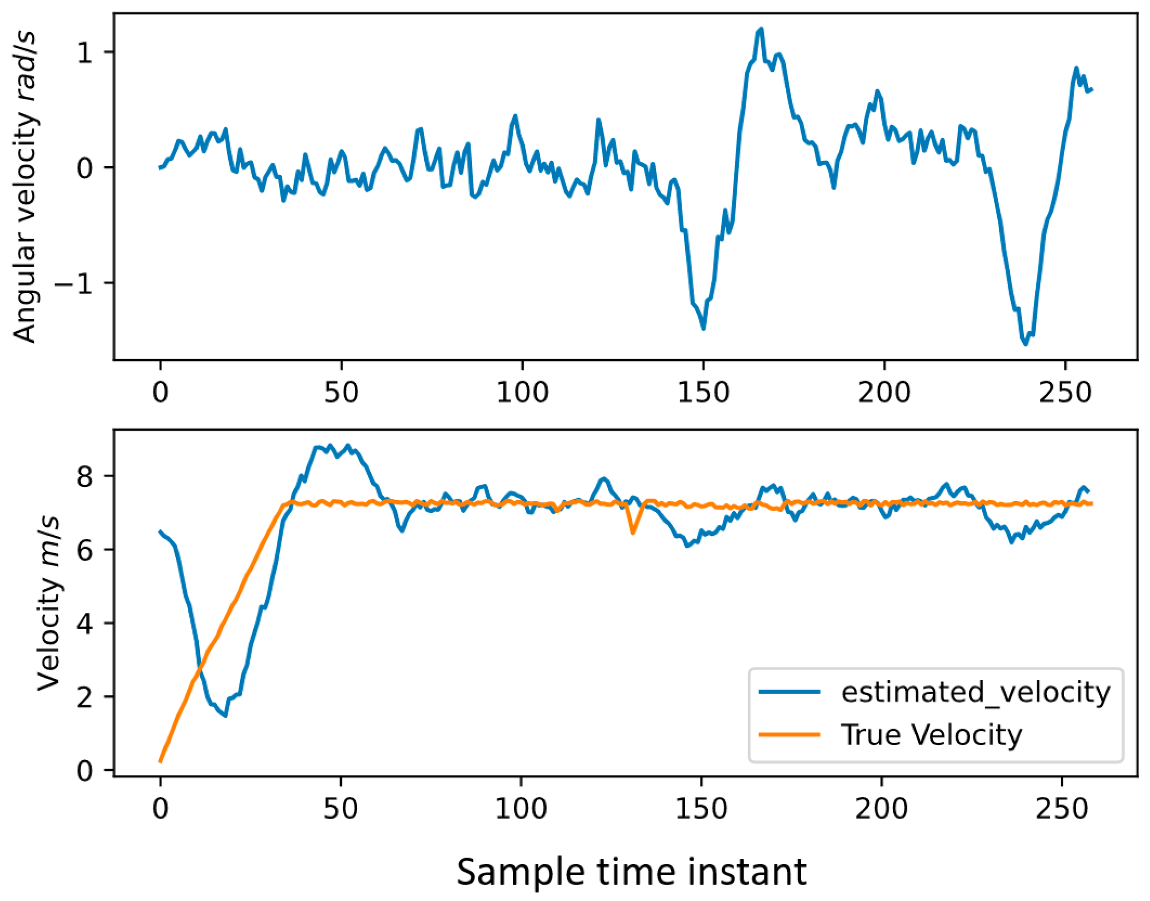
2.3. Simulation Experiment Setup and Results

This study was motivated by the presence of two round intersections in the Linden LEAP autonomous shuttle deployment site of Columbus, Ohio, as part of the Smart Columbus project (US DOT Smart City Challenge award) [20]. The Linden LEAP AV shuttles operated in an urban city environment with no public transportation and picked up and dropped off passengers at the four stops of the Linden Transit Center, Rosewind Estates Community Center, Douglas Community Recreation Center, and St. Stephen’s Community House. These locations provided residents with resources that include affordable housing, healthy food, childcare, healthcare centers, recreation, and more. It also connected residents who live in the area to the Central Ohio Transit Authority’s (COTA) CMAX rapid transit bus line to access jobs and services. The AV shuttle route had two round intersections. The shuttles used were not able to autonomously handle the round intersections. Instead, the shuttle operator monitored the traffic situation in the round intersection and pressed the proceed button for the shuttle to automatically track its path within the round intersection. The round intersection geometry and speeds used in the simulation experiments correspond to this autonomous shuttle deployment. These AV shuttles had a maximum speed of about 3.6 m/s (8 mph).
The experiment of implementing UKF for vehicle trajectory tracking is tested based on simulation trajectories generated in the SUMO microscopic traffic simulation environment. The vehicle model for unscented Kalman filter-based vehicle trajectory tracking is the CTRV model introduced in this section. Here, we use one of the experiments for demonstration and show the test results based on SUMO simulation. A vehicle in SUMO travels around the round intersection and generates the path shown in Figure 1. To simulate the noisy process of the vehicle state transition and the noise generated in the process of measurement, we manually add process noise and measurement noise to the clean trajectory. As was shown in Equation (9), we add a white noise on the velocity and angular velocity as follows:
v a v w t N μ , cov ( v )
where μ = 0 0 and cov ( v ) = σ v a 0 0 σ v w with σ v a = σ v w = 0.01 . Each vehicle passes the roundabout intersection, and the clean trajectory is shown in Figure 2.
We also add white noise to the measurement. In the experiment, the measurement is [ x , y , θ ] , that is, vehicle position and its heading angle. The measurement noise is set as
n x n y n t h e t a t N μ n , cov ( n )
where μ n = 0 0 0 and cov ( n ) = σ n x 0 0 0 σ n y 0 0 0 σ n θ , σ n x = σ n y = σ n θ = (0.5)2. The result of the testing is shown in Figure 3. The clean trajectory is recorded from vehicles in SUMO simulation environment is shown as a green line, and the processed noisy trajectory is shown as a blue line, while the red line shows the filtered trajectory process by the unscented Kalman filter. In this trajectory filtering, it is easily seen that the measured trajectory is noisy for the lateral and longitudinal positions, and the filtered trajectory can remove noise to some extent and converge to the clean trajectory. The filtered trajectory fluctuates the most at the part of the path where the vehicle is turning, and it takes longer for the filtered trajectory to converge at the cornering point. It is seen that the error can reach up to 0.5 m. at such points, which is significant. The results of the estimation of hidden states of vehicles, such as velocity and angular velocity, are shown in Figure 4.
In the SUMO environment, the vehicle’s speed is accessible. Hence, we use it for comparison to illustrate the performance of the UKF-based vehicle trajectory estimation. The initial condition set for estimation is the normal driving speed of the vehicle. Hence, it starts with large errors. However, it converges to the true velocity soon and tracks the true velocity, which is like the Linden LEAP AV shuttle speed with a factor of safety of two. The allowed speed limit at an intersection is usually 15 to 25 mph, which corresponds to 11 m/s as an upper speed limit. If the upper speed limit is increased further and considered as 30 mph using a factor of safety of two over the 15 mph limit, the corresponding speed in m/s will be 13.4 m/s, which is considerably higher than the maximum speed seen in the simulation results here. The methods presented here can be applied to such higher speeds after re-defining the round intersection geometry such that these larger speeds can be accommodated with reasonable levels of lateral acceleration. The computations would need to run faster for real-time implementation due to the larger speeds involved. The estimation of the angular velocity is also presented in Figure 4. We do not have access to the angular velocities of other vehicles. Hence, the UKF-based state estimation provides a tool for estimating the hidden states such as angular velocity. This test has been conducted for three vehicles’ trajectories in the simulation and the test results are listed in Table 1. A large initial estimate error is used in the simulation experiments on purpose to show that the UKF converges fast to the actual state. Larger process and measurement noise will degrade the results of the UKF and other similar filters and can be used to investigate the sensor characteristics for desired performance.

3. Change Point Detection-Based Behavior Prediction

In this section, a policy prediction method leveraging Bayesian change point detection technique is introduced. This method was first introduced in [21] for determining the current behavior of the observed vehicles and to detect anomaly behavior performed by them during highway driving. This method is modified here by introducing the Kalman filter-based state estimation for generating a clean vehicle trajectory history for assisting the behavior prediction and a new method for solving the computation of likelihood value for different vehicle policies under the scenario of the round intersection. Our modified method also predicts the future dynamic behavior of the observed vehicle using the vehicle hidden states estimated by the Kalman filter with the CTRV model. In the previous work of [21], which is used in the derivations here, the authors presented an integral method for decision making with behavior detection. In this paper, we just utilize the method for behavior prediction and combine it with vehicle motion model for predicting vehicle behavior in the near future so that the estimated trajectory derived from the prediction method can assist a decision-making algorithm.

3.1. Problem Formulation for Vehicle Behavior Prediction

In the urban traffic scenario, vehicles around the ego vehicle will behave differently to respond to the current traffic situation, which makes it a complex task for the ego autonomous vehicle decision making for efficient and safe driving. Hence, it is very helpful to have good prediction of other vehicles’ trajectories and behaviors within the observation range of the ego vehicle. Let V denote the set of vehicles near the autonomous ego vehicle within its range of on-board sensors. Also include the ego vehicle in the set by letting v e represent the ego vehicle and v i , i { 1 , , n } represent the n surrounding vehicles such that all the vehicles considered are in the set V, and the set is V is as follows:
V = { v e , v 1 , v 2 , , v n }
Each v i V is described by a five-tuple of state vectors s i = ( x , y , θ , v , w ) i that represents planar position of the vehicle on the road, heading of the vehicle, and also motion variables linear velocity v and angular velocity w . At each time t, vehicle v i will select an action a t v i A from an action set to drive the vehicle and update its state vector from s t i s t + 1 i . Both of the states are included in the set of states S .
The vehicle motion model is represented by a conditional probability function T and is as follows:
T ( s t , a t , s t + 1 ) = p ( s t + 1 | s t , a t )
Note that s t S includes all the state of the vehicles in the vehicle set V, and similarly, a t A denotes all the actions that vehicles might take at time t. Observations with uncertainty on the vehicles in V are also modeled as follows:
Z ( s t , o t ) = P ( o t | s t )
where o t is the observation and is also the set of observations that the ego vehicle can acquire through the on-board sensors. Each of the observations made over the individual vehicles v i is o t i . Due to the diversity of sensor systems, the observations of other vehicles are also various and need to be processed. In this section, measurements and observations are not the critical part. Hence, the observation and the processing of the observation will not be covered here. As was presented in the previous section, the observation used for this part is just partial vehicle state information and hidden variables such as angular velocity of other vehicles that are not accessible from the ego vehicle. Drivers of the vehicles tend to drive in the manner that maximizes some driving demands that can lead to the goal destination or speed in the shortest time. There are also uncertainties contained in the driving behaviors. The driving model is represented as follows:
D ( s t , o t i , a t i ) = p ( a t i | s t , o t i )
The model in (18) shows that the driver’s behavior is based on current states of all the vehicles and the observations made. Considering the uncertainties of the vehicle states, the vehicle state at time t is modeled and represented by probability distribution P ( s t i ) , for   i = 1 , , n . The overall states for all the vehicles in V are shown as P ( s t ) . While vehicles are driving on the road, the states keep transforming based on the transition function T, the observation function Z, and the driver model D as follows:
P ( s t + 1 ) = X O A P ( s t + 1 | s t , a t ) P ( a t | s t , o t ) P ( o t | s t ) P ( s t ) d a t d o t d s t
The set S refers to all the states of the vehicles in the vehicle set. O represents the set of observations, and A contains all the possible actions that the vehicle can take under traffic scenarios. With the assumption that each of the vehicles in the set are independent from others, (19) can be transformed as follows:
P ( s t + 1 ) = v i V p i ( s t + 1 i , s t i , a t i , o t i ) d a t i d o t i d s t i
p i ( s t + 1 i , s t i , a t i , o t i ) = P ( s t + 1 i | s t i , a t i ) P ( a t i | s t i , o t i ) P ( o t i | s t i ) P ( s t i )
to predict the future state distribution P ( s t + 1 ) , and the prediction of driver model D ( x t , o t i , a t i ) = p ( a t i | x t , o t i ) is the main task to solve in this section.

3.2. The Multipolicy Approach for Driver Model Prediction

As discussed in [21], traffic participants will commonly behave in a regular and predictable manner and do not seem to change in a quick, sudden manner such that other vehicles cannot respond. The vehicle motions cannot be changed without any preceding stages either. It would be a good idea to leverage the vehicle state trajectory in a period of timestamps and persuade the possible vehicle behavior out of the observed vehicle trajectory. Then, one should find the maximum a posteriori (MAP)-estimated policy based on likelihood estimation.
The prediction is based on latent vehicle policies that the vehicle on the road can possibly take for driving. A vehicle tries to achieve the goal of driving. This goal can be quantified as the real-time reward function:
r : S × A R
The reward function depends on the demand of the vehicle. Based on vehicle drivers’ demand on the road, it may be related to safety issues, velocity, comfort, and time to destination or other concerns that vehicles and their drivers have on the road. A policy is a mapping of the current state of the vehicle, the current observation of the available action set is as follows:
π : S × Z A
An optimal policy is the policy that maximizes the expected sum of real-time reward over some time horizon, H, as given by the following equation:
π * = arg max π E [ t = t 0 H R ( s t 0 , π ( s t , o t ) ]
For the decision-making problem, the goal of finding the optimal policy is to make sure that the vehicle can drive safely and efficiently. In this section, the goal, instead, is to estimate the most likely policy that the observed vehicle is taking.
To make this estimation problem tractable, as discussed in the previous part, a set of latent discrete policy will be introduced first. The policy set contains the policy that covers hand-engineered policies specifically designed for the target traffic scenario. Here, the policies in the set are high-level vehicle control policies that provide instructions to the vehicle on what kind of behavior they should perform. An explicit low-level control should be applied for policy execution. This allows a broad range of control algorithms to be implemented and is not in the scope of this paper.
Let us assume that each vehicle v i V , at any time of driving under the current traffic scenario, is executing some policy from the pre-defined policy set, expressed as follows:
π i   for   i = 1 , 2 , , n
where π i is the policy that vehicle v i is currently executing, and n is the number of vehicles that are not the ego vehicle in the set. In general, the policy itself can be parametrized as a function with respect to current states of the whole set of vehicles s t , including the observed states and hidden states within the state vectors, as well as the parameter vector θ i . This parameter vector can be used for capturing the features of driving, for example, the aggressiveness of the driver. The dynamic limit of the current observed vehicle may lead to different types of vehicle state trajectories under the same policy from the set. Since the action the driver selects is generated from the policy, the driver model of vehicle v i in Equation (18) is now expressed as follows:
D ( s t , o t i , a t i , π t i ) = P ( a t i | s t , o t i , π t i ) P ( π t i | s t , o 1 : t )   for   i = 1 , 2 , , n
The first part shows that the action the driver might take depends on the current state of all the vehicles, considering both other vehicles and the ego vehicle, as well as the observations and policy. The policy is determined by the current state with the series of observation o 1 : t . The derivation of the conditional probability P ( π t i | s t , o 1 : t ) is the core problem to be solved in this section, and its solution will be presented later in this section. Updating the driver model based on policy, the state probability distribution evolution equation shown in Equation (21) can now be approximated as follows:
p i ( s t + 1 i , s t i , a t i , o t i , π t i ) = P ( s t i ) P ( o t i | s t i ) P ( s t + 1 i | s t i , a t i ) P ( a t i | s t i , o t i , π t i ) P ( π t i | s t , o 1 : t )
The overall state probability distribution is then a joint-probability distribution between the state distribution of the ego vehicle and other vehicles in the set, and is as follows:
P ( s t + 1 ) = P ( s t + 1 e , s t + 1 v i ) , i = 1 , 2 , , n   and   v i e
P ( s t + 1 ) = S e O e P e ( s t + 1 e , s t e , a t e , o t e , π t e ) d s t e d o t e v i V , v i e S v O v P v i ( s t + 1 v i , s t v i , a t v i , o t v i , π t v i ) d s t v i d o t v i
The ego vehicle is assumed to be in full control. Therefore, the state distribution update can be derived based on the policies determined with the decision-making algorithm implemented for the ego vehicle.
The future states of other vehicles depend on their own policies that we do not know. Thus, the policy shall be predicted for the conditional probability as follows:
P ( π t i | x t , o 1 : t )
Then, a forward simulation with corresponding low-level controller and appropriate motion model shall be carried out to obtain the future trajectories based on the current estimated policy. The trajectory prediction method here utilizes a Bayesian change point detection method, leveraging the measured trajectories of the target vehicle. To segment a tracked vehicles state trajectory over a past period of time, the change point detection method proposed in [22], Change Point Detection using Approximate Model Parameters (CHAMP) algorithm, is adopted since it takes advantage of the feature of change point detection and applies it to segment data that are not only generated from random processes, but data obtained by observing different types of vehicle motion. Since the vehicle motion is continuous, without sudden jump, if the vehicle is executing some policy in a segment of the trajectory, the change in policies can be detected given a set of available policies and a series of observed data of given vehicle, denoted as o 1 : n = { o 1 , o 2 , , o n } .
The CHAMP algorithm infers the maximum a posteriori (MAP) set of times, τ 1 , τ 2 , , τ m , at which change points between policies have occurred, and this will segment the time series into m + 1 data segments corresponding to policies executed on those data segments. The i t h observation segment o τ i + 1 : o τ i + 1 is detected associated with a certain policy from the pre-defined policy set. In the following part, the CHAMP algorithm is introduced and illustrated as to how it works for detecting the change point between different data associated with corresponding policies.
The change point positions are also described by probability distribution and can be viewed as a Markov chain where the transition probabilities between neighboring change points are a function of time as follows:
P ( τ i + 1 = t | τ i = s ) = g ( t s )
The probability distribution function (pdf) g ( · ) is a function over the length of the data segment, and we denote the cumulative probability distribution (cdf) of the function g ( · ) as G ( · ) . In the algorithm of CHAMP, the truncated Gaussian function over the length of data segment is used as follows:
g ( t ) = 1 σ ϕ ( t μ σ ) 1 Φ ( α μ σ )
G ( t ) = Φ ( t μ σ ) Φ ( α μ σ )
where ϕ is the standard normal distribution pdf, Φ is its cdf, and α is a parameter that should be defined based on different cases for using this change point detection algorithm [22].
Another important factor for segmenting data based on different policies is the confidence that the series of data is generating under the policy π , defined as policy evidence, and is as follows:
L ( s , t , π ) = P ( o s + 1 : t | π ) = P ( o s + 1 : t | π , θ ) p ( θ ) d θ
In the above equation, the confidence of policy π over the data segment starting from time s to time t is shown. For the purpose of efficient computation and avoiding marginalizing over the parameters in the conditional probability of policy, CHAMP makes an approximation by using logarithm of the policy evidence via the Bayesian Information Criterion (BIC) and is as follows:
log L ( s , t , π ) log P ( o s + 1 : t | π , θ ^ ) 1 2 k π log ( t s )
where k π is the number of parameters for the policy π depending on the type of pdf describing the policy function. θ ^ are the estimated parameters for policy π . This BIC approximation for policy evidence does not require marginalizing of the probability over the parameter and it penalizes the complexity of the model with the part 1 2 k π log ( t s ) , with respect to the parameters of the model. Another advantage of using this BIC for computing the policy confidence is making full use of the series nature of data since the BIC equation of (35) is only applicable when the size of data is way larger than the number of parameters. The computation of BIC only requires fitting different policies into the observed data segments and obtaining the maximum likelihood estimation (MLE).
According to [23], the distribution C t over the most recent change point before time t can be estimated by regaining the Viterbi path by applying an online Viterbi path algorithm and Bayesian filtering recursively. A Viterbi path is the path of the maximum posteriori probability estimate of the most likely sequence of hidden states [24]. In our case, the hidden state is the change point detected. The terms and definitions used for finding the MAP of the most recent change point before time t are provided next. The probability distribution
P t ( j , π ) = P ( C t = j , π , ε j , o 1 : t )
is the probability of the last change point that occurs at time j before t, associated with policy π given by
P t M A P = P ( CP   at   t , ε t , o 1 : t )
which shows the maximum a posteriori choice of a change point occurring at time t . Equations (36) and (37) result in the following:
P t ( j , π ) = ( 1 G ( t j 1 ) ) L ( j , t , π ) P ( π ) P j M A P ,
P t M A P = max j , π g ( t j ) 1 G ( t j 1 ) P t ( j , π ) .
ε j in the above equations represents an event where the change point based on MAP choice occurs prior to time j provided the condition that the change point is at time j. At any time t in the time series, the Viterbi path can be recovered by maximizing the MAP choice P t M A P with respect to the pair ( j , π ) as j is the one step previous change point for the data. The whole process will keep repeating until the first data point of the whole data series is reached. The Viterbi path consists of all the change points that are derived from the optimization process. The change point will be used as the index for segmenting the data into segments.

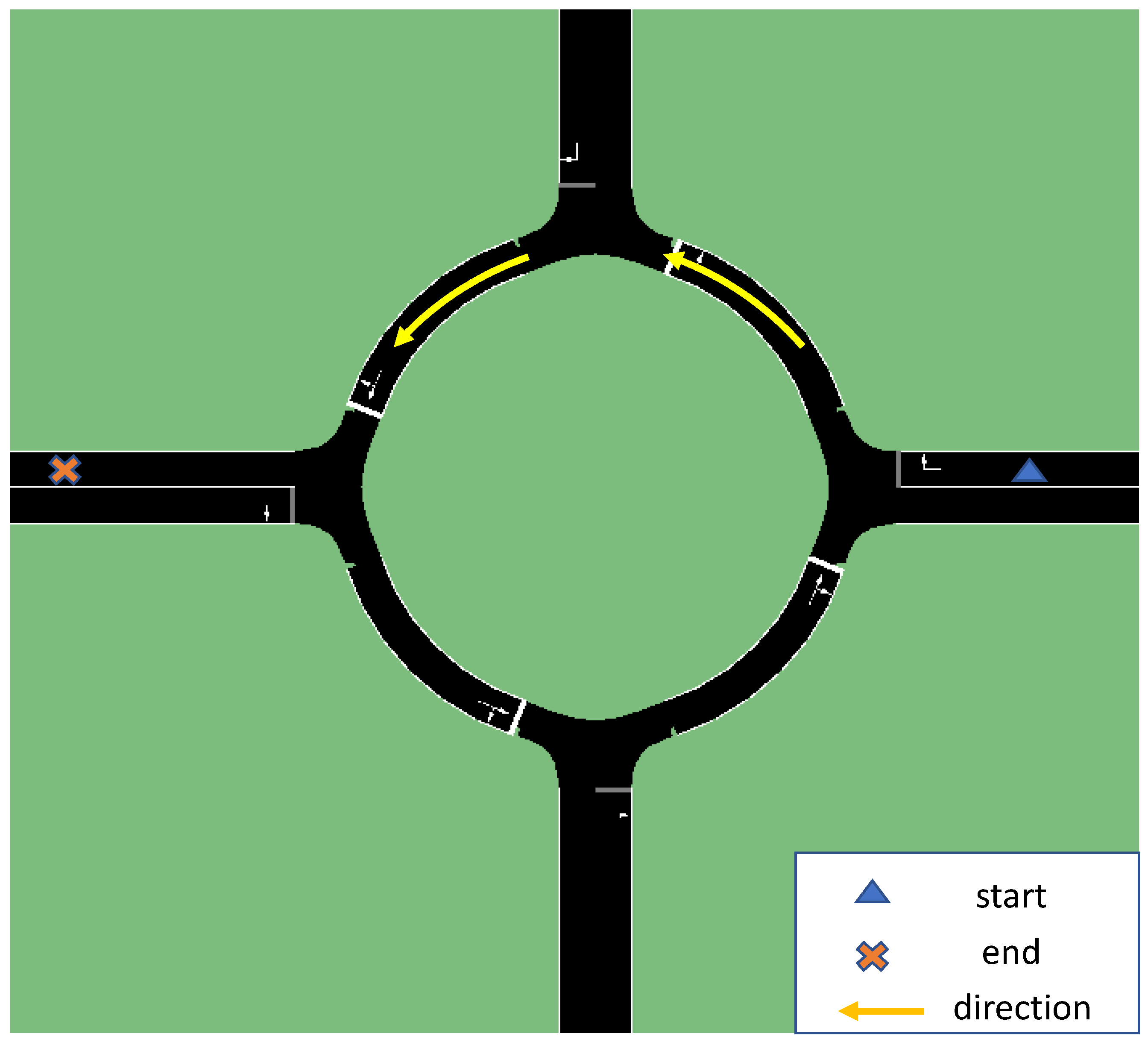
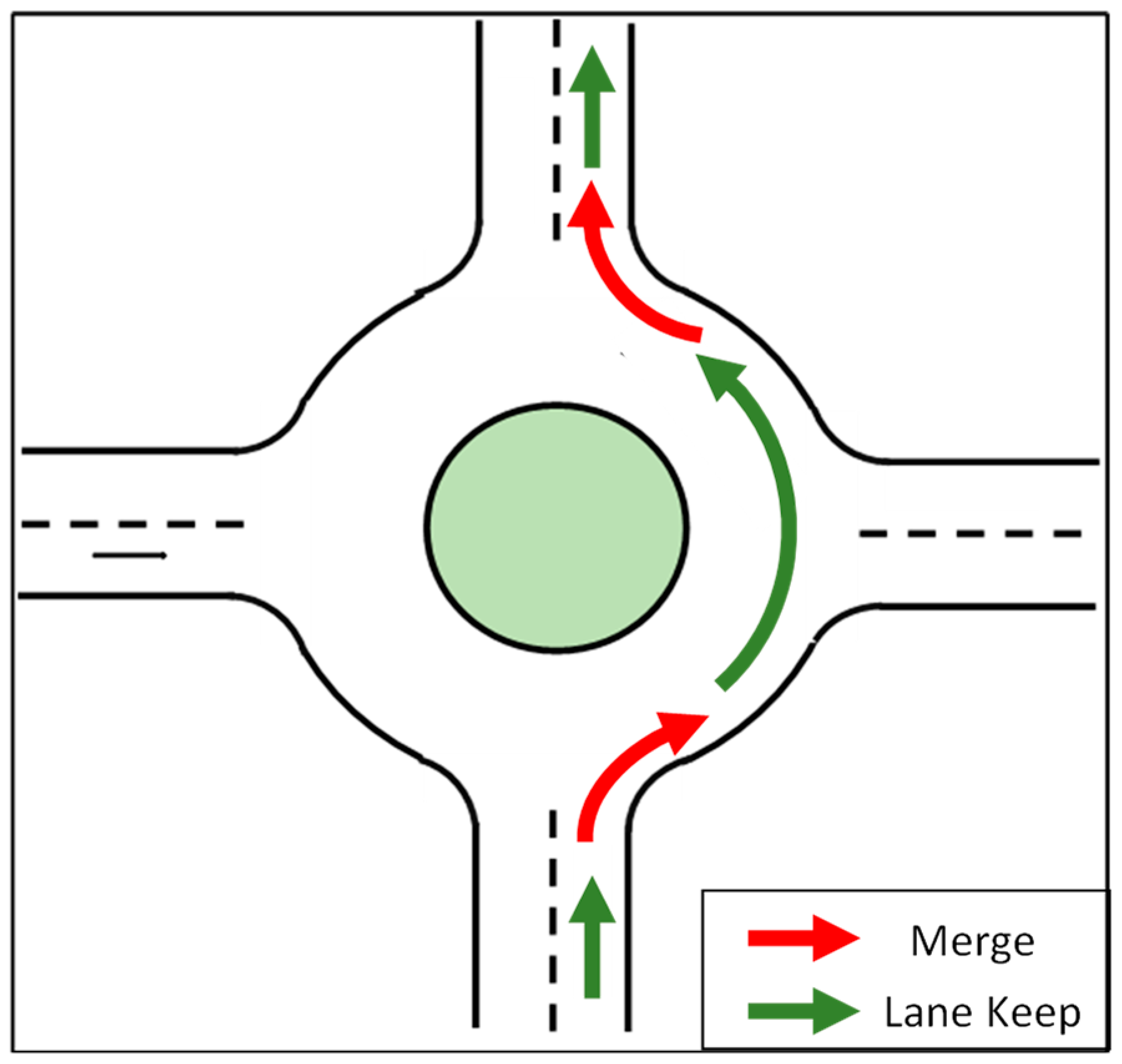
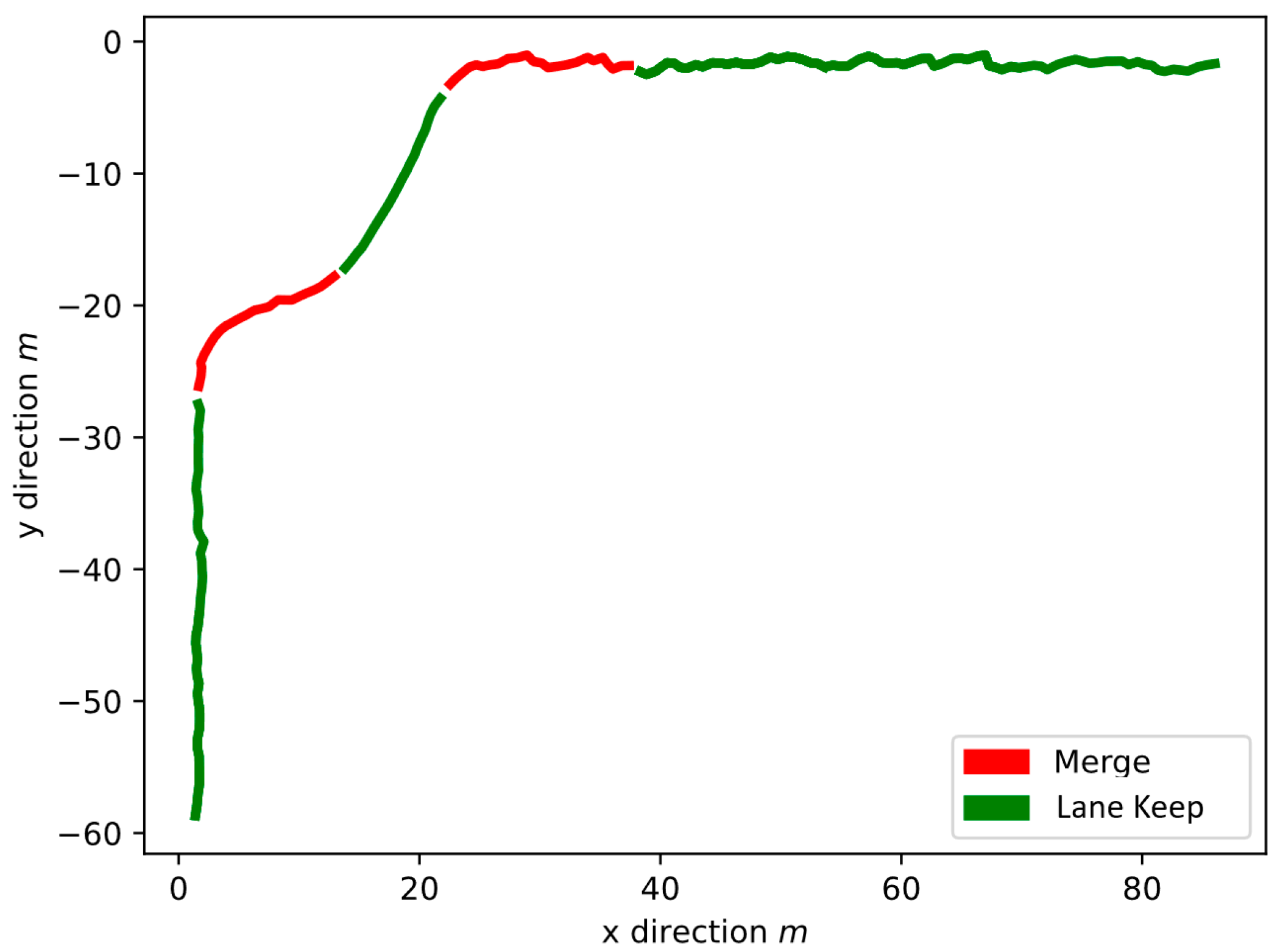
3.3. Behavior Prediction for Round Intersection

In this part, the task of predicting vehicle policy in the round intersection is presented, and the solution for estimation is shown for a round intersection. Similar to the method proposed in [21], the way of fitting policy to a specific data segment is based on the likelihood value of different policies. The policy evidence or the policy confidence, as is introduced in previous context, is the core item for determining the associated policy of a given data segment. Note that a series of vehicle state data observed from a vehicle v described the partial state trajectory as o 1 : t = { o 1 , o 2 , , o t } . Given that the trajectory has been detected and m change points have been detected, the last data segment in the data series is o m + 1 : t . Based on Equations (34) and (35), the policy likelihood for the given data segment can be computed as follows:
L ( π ) = max π , θ ^ P ( o m + 1 : t | π , θ ^ )
log L ( π ) = max π , θ ^ log P ( o m + 1 : t | π , θ ^ )
The posterior probability of the maximum likelihood estimation is derived with the observed data series and the forward simulation of vehicle trajectory under certain policies.
The forward simulation of a vehicle generates a future potential trajectory provided π , and it takes advantages of the typical geometry structure of a round intersection. A round intersection can be decomposed into three main parts, the straight lanes connecting to the roundabout, the part of road where the straight lanes are connecting to the round intersection, and the round intersection, and vehicles will behave differently during the drive on those three types of road segments. To be clear, the vehicle policies during in-lane driving or highway-like driving are not considered in this paper, and vehicle behaviors such as lane changing are not the goal for prediction. Mainly, two kinds of policies are to be predicted. When the vehicle is driving in-lane, no matter on a straight road or in a round intersection, the vehicle behavior is defined to be under the policy of lane keeping. When the vehicle is trying to enter a round intersection or trying to leave from the round intersection into a straight connected road, the policy is defined to be merge, which means the vehicle is getting in contact with the connection point between the round intersection and the straight road and approaching a different type of road. Hence, the whole policy set with the driving style as the parameter is given by the following:
{ l a n e   k e e p   m e r g e }
Different policies in the policy set are shown below in Figure 5. In Figure 5, a vehicle is passing a round intersection starting from the bottom of the figure and moving to the top of the figure along the round intersection. The vehicle first drives in the straight road segment, then merges into the round intersection. After entering the round intersection, it follows the single lane in it until it reaches the target exiting area to exit it and merges back to the straight road segment. The whole process can be divided into five sub-segments as shown in Figure 5, and can be described by the policies in (42) as the following sequence:
{ l a n e   k e e p } { m e r g e } { l a n e   k e e p } { m e r g e } { l a n e k e e p }
To be easily noted, the segments with policy l a n e   k e e p are colored green and those with policy m e r g e are colored red in Figure 5.
The likelihood computation, as shown in Equations (40) and (41), is approximated by finding the likelihood value based on normal distribution with the observed trajectories as parameters in the following equation:
P ( o m + 1 : t | π , θ ) = N ( o m + 1 : t ; T π , θ , σ I )
Yet, the observed trajectory is a series of state vectors. Each state vector, based on the observation model, should contain vehicle pose information. In this paper, the observation of other vehicles is O t v = ( x v , y v , θ v ) , in which longitudinal position is x v , lateral position is y v , and heading angles of the vehicle are θ v . Hence, fitting the whole series of observed state trajectory into the normal distribution will lead to a matrix Gaussian distribution and requires computation for high dimensional data. To make the computation more efficient, we made an approximation such that the correlation between the three state variables are ignored, and the whole state trajectory is split into three trajectories containing x v , y v , and θ v , denoted as T x v π , θ , T x y π , θ , T θ v π , θ . Therefore, Equation (41) is represented as follows:
log L ( π ) = max π , θ ^ log P ( o m + 1 : t | π , θ ^ ) max π , θ ^ log P ( x v , m + 1 : t | π , θ ^ ) + log P ( y v , m + 1 : t | π , θ ^ ) + log P ( θ v , m + 1 : t | π , θ ^ )
π v ^ * = arg max π log L ( π )
By computing the log likelihood value as the BIC, the segments will be determined with the policy most likely π v ^ * from the policy set.

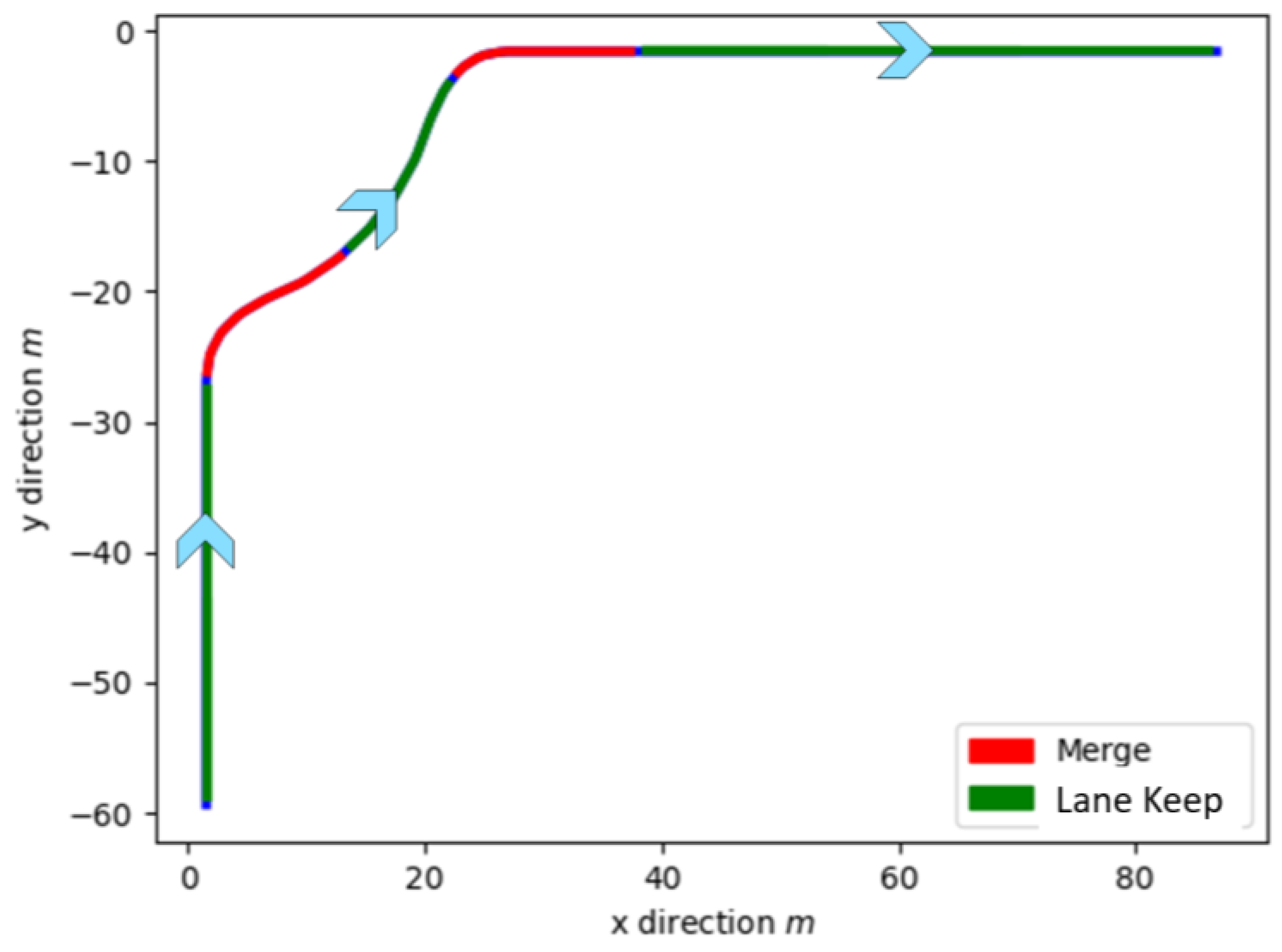
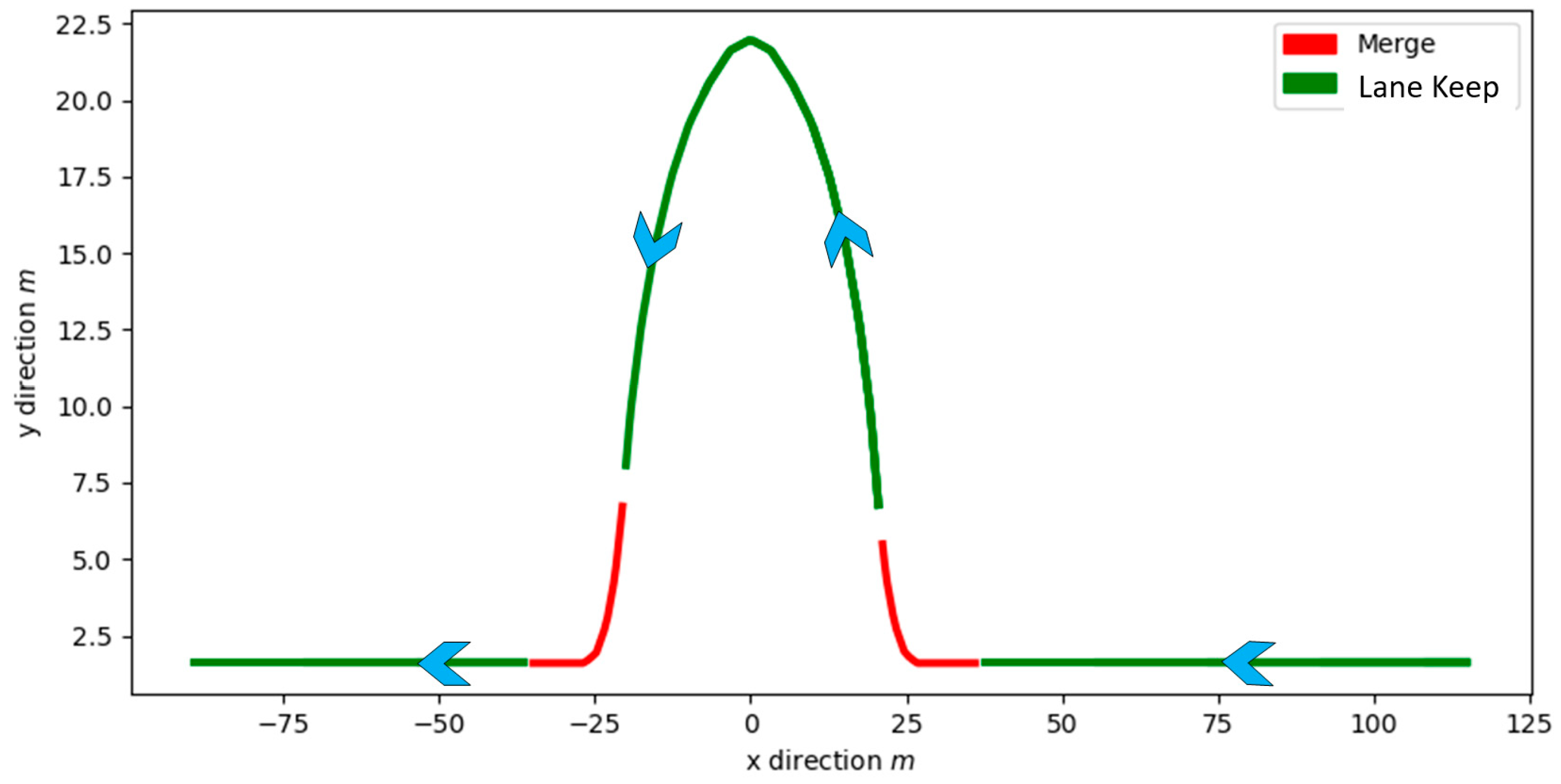
3.4. Simulation and Test Results of Policy Prediction

In the simulation test, the policy prediction method is used to determine the vehicle’s policy in different trajectory segments given a series of vehicle trajectory data. In this work, the tests have been conducted on clean trajectory directly collected from SUMO environment and the noisy trajectory obtained by adding measurement noise to the clean trajectory. The results are shown in Figure 6 and Figure 7 and are discussed below. First, the results on policy prediction based on change point detection are presented. Same as the previous section, the tests are on recorded clean vehicle trajectory passing a roundabout intersection. The vehicles, based on the trajectory data, are determined for executing a policy from the policy set. For the test, the set of parameters for the change point detection-based policy prediction is also required. For the segment length distribution in Equations (32) and (33), the mean length of the segment is set to be 50, and the minimum segment length is set to be 25. The result of the prediction is shown in Figure 6 and Figure 7. The vehicle travels following the direction of arrows. At the cornering part where vehicle is entering or exiting the round intersection area, the policy prediction algorithm correctly determines the policy to be merge. In the other parts of the trajectory, the vehicle policy is correctly determined to be lane keep.
After adding the measurement noise to the trajectory data, the policy prediction is influenced by the oscillation of the vehicle trajectory as shown in Figure 8. Due to the noise in the trajectory, policy prediction cannot work properly and will cause some error and may miss the policy change between different trajectory segments as seen by comparing Figure 6 with Figure 8. Hence, we introduce the Kalman filter for filtering out the noise along the trajectory and make sure the prediction method can work well when there is noise in the measurement in Figure 9. With the UKF, the prediction method can work better with noisy measurement of other vehicles’ trajectories as shown in Figure 9.

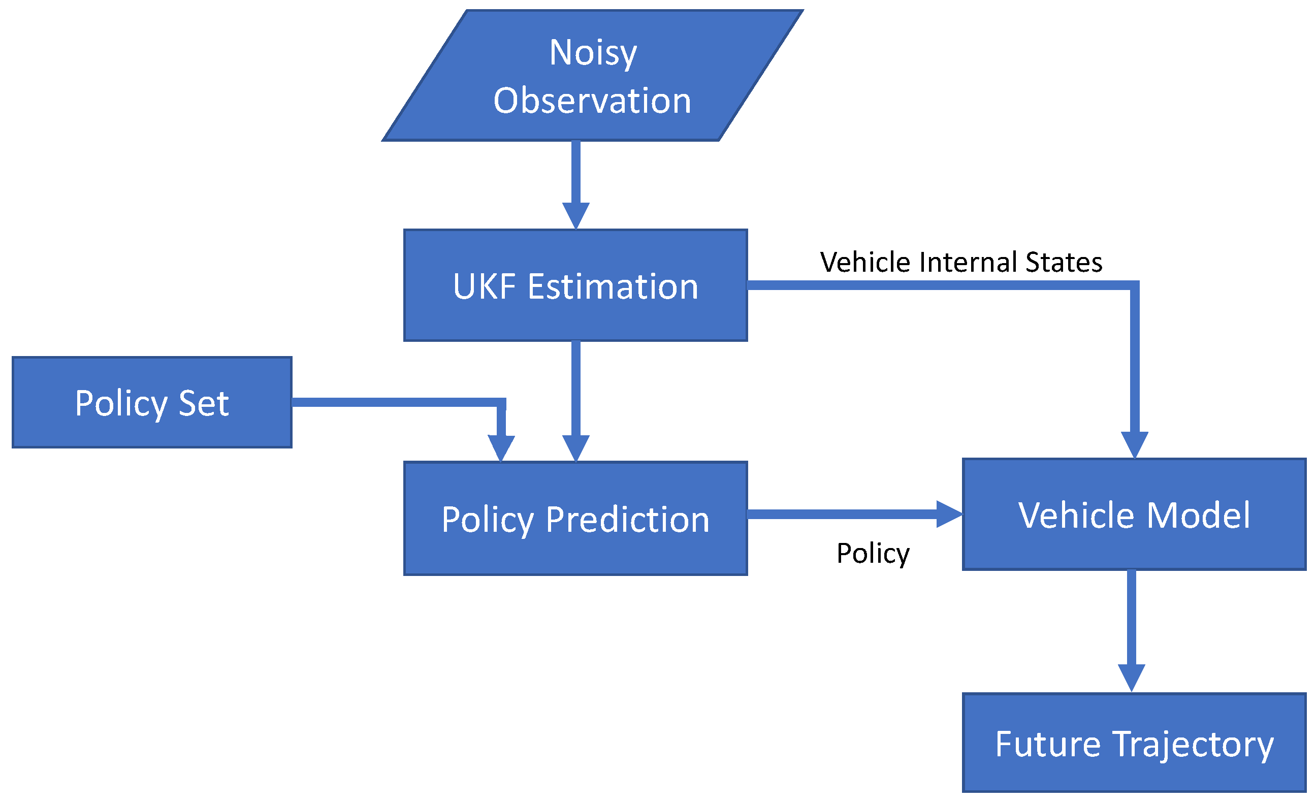
4. Vehicle Trajectory Estimation Based on UKF and Policy Prediction Method

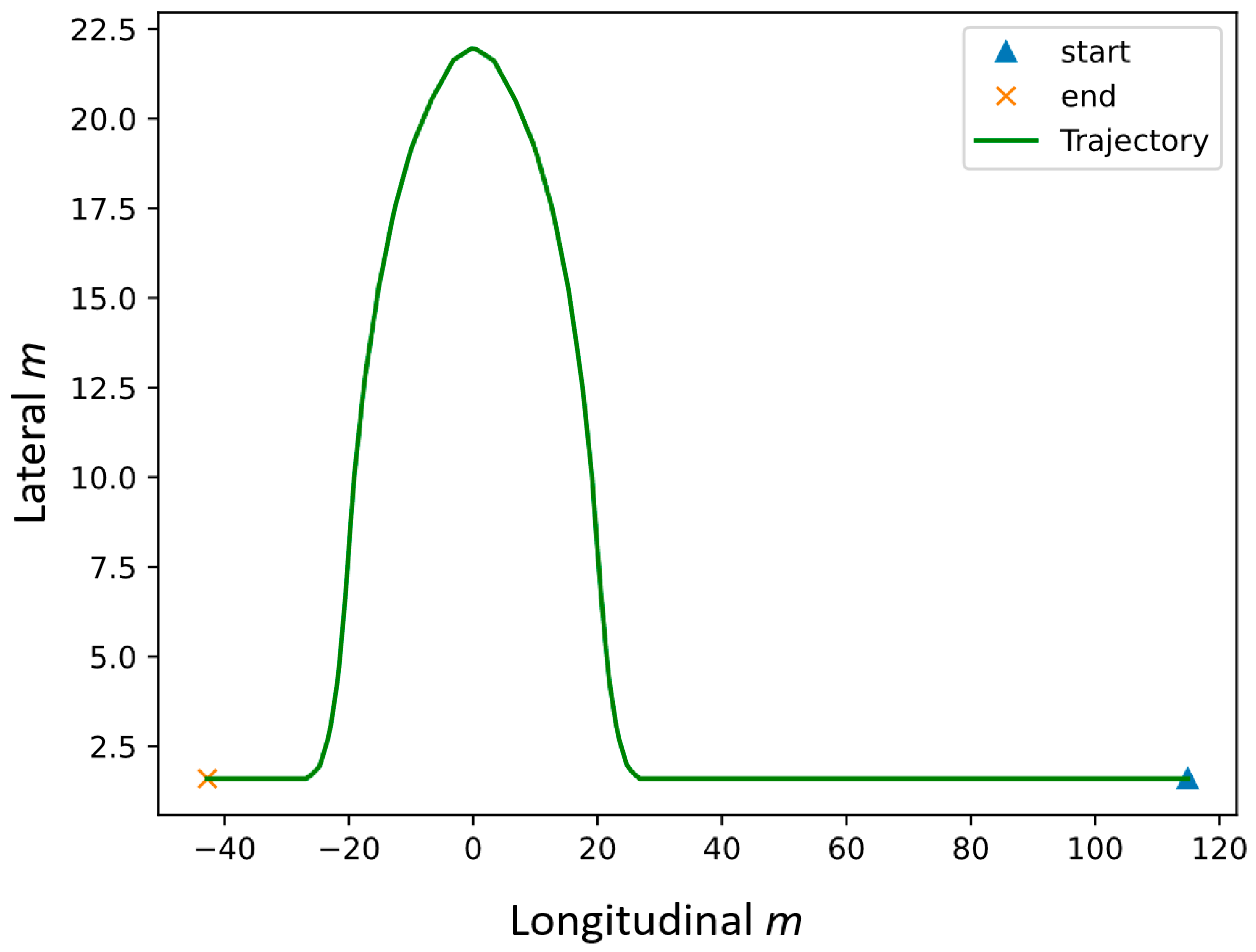
4.1. Vehicle Trajectory Estimation

In Section 2 and Section 3, the state estimation based on the unscented Kalman filter for unobserved internal state variables with noisy measurements and the policy prediction of the vehicle based on change point detection method were presented, respectively. In this section, we introduce the method for vehicle trajectory prediction over a future period of time for a target vehicle. The whole workflow is shown in Figure 10.
The existence of the UKF estimation allows the trajectory prediction system to predict a reasonable future trajectory. Even when there are some anomalous policies, the corresponding trajectory can be retrieved. The forward simulation for determining the prediction utilizes the known geometry feature of a round intersection. Given the CTRV model, the angular velocity is different at different parts of the round intersection including the entering and exiting areas. The angular velocity will change during the policy execution for the policy m e r g e . In contrast, the vehicles’ angular velocity will remain the same for the whole stage of the policy l a n e   k e e p . This provided us the key point of generating different simulation trajectories based on different policies.

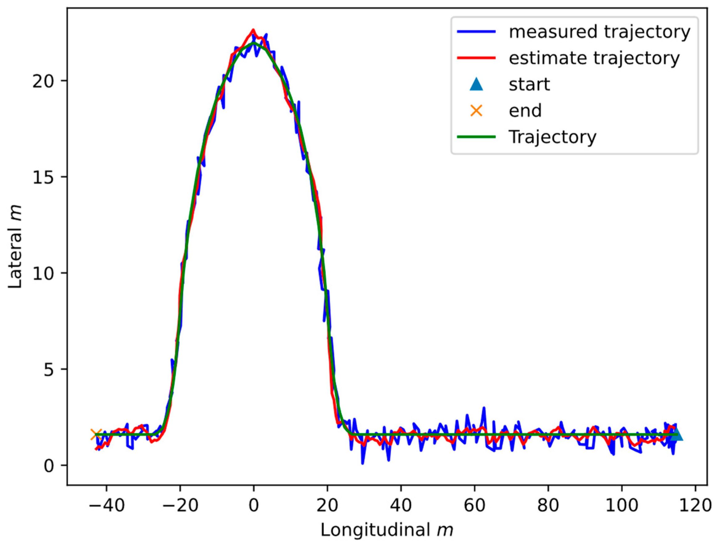
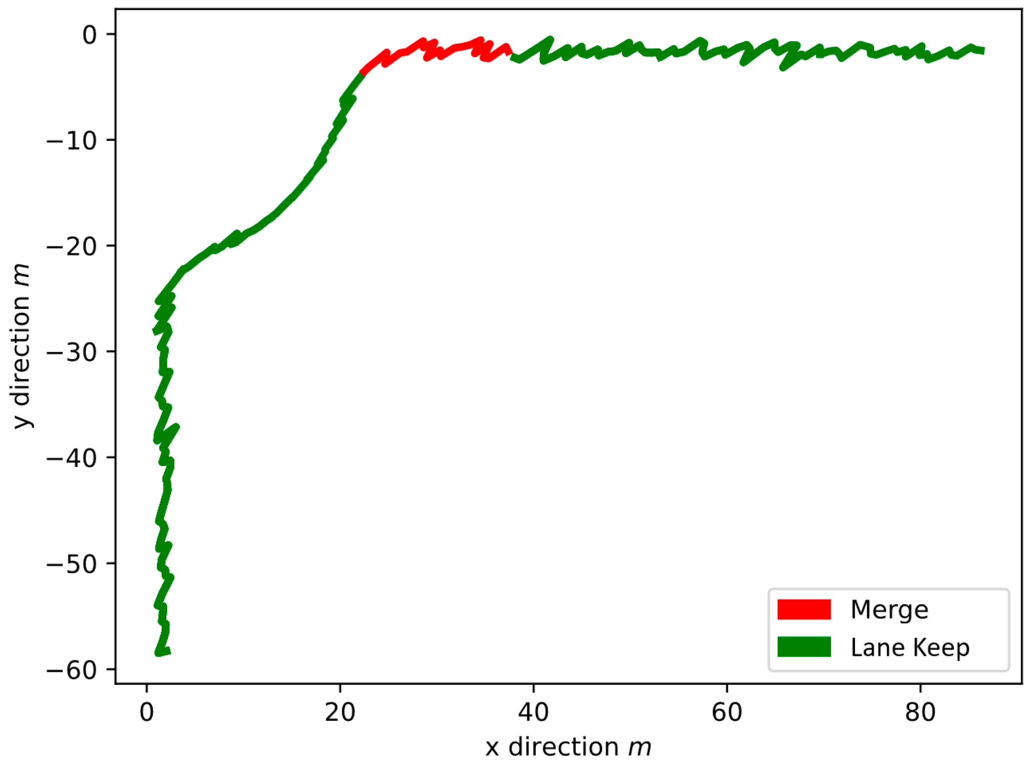
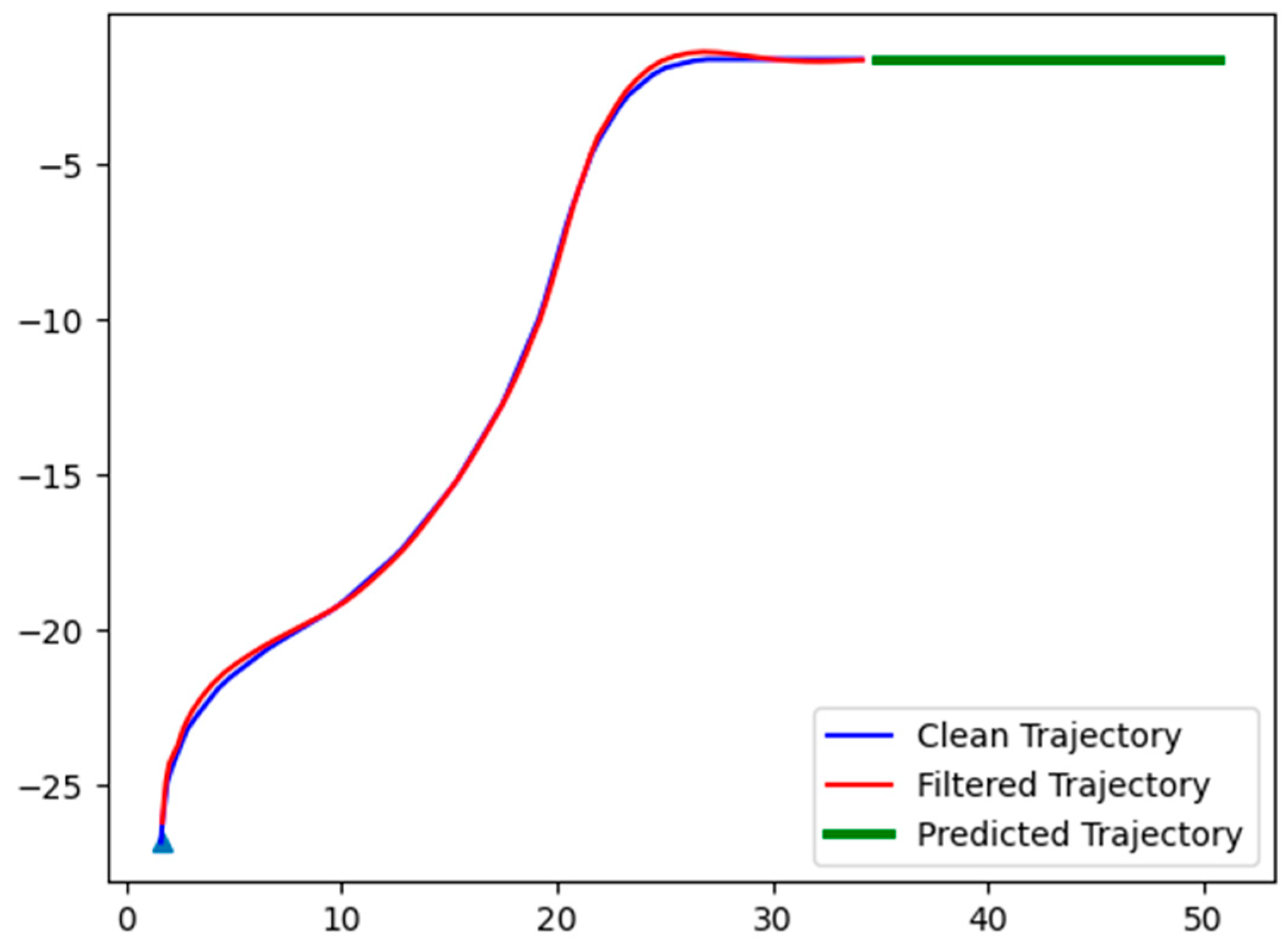
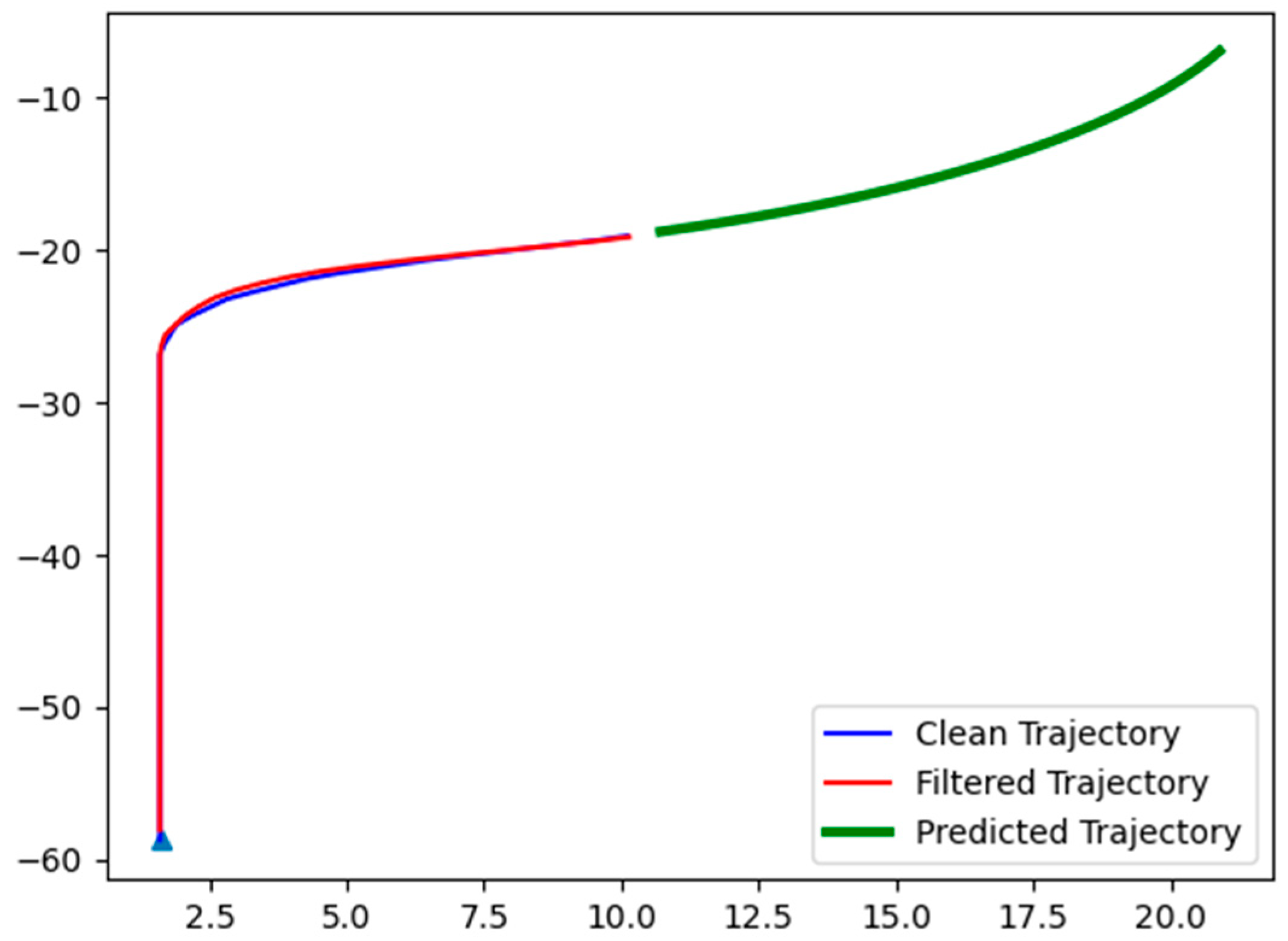
4.2. Test Results on the Vehicle Trajectory Estimation Method

In this section, several test results for vehicle trajectory prediction are presented. In Figure 11, a vehicle trajectory estimation result is shown. The vehicle is moving from bottom to upper right of the figure and with the last state estimated with UKF and the policy prediction result of the policy is { l a n e   keep } , the predicted trajectory (shown in green) is generated. With the observed trajectory, the agent vehicle does not have the information about angular velocity; hence, the UKF estimates this hidden state and provides a direction of vehicle moving forward. In Figure 12, the vehicle trajectory prediction is for the vehicle within the traffic circle, with the estimated vehicle states, and the trajectory prediction method is able to forward simulate the potential vehicle path in the round intersection.
The proposed change point detection with Kalman filter approach can be compared to the Kalman filter (UKF) approach alone in the paper by comparing the results in Section 4 and Section 3 where the Kalman filter results are representative of other published approaches in the literature. The comparison shows the improvement offered by the proposed method.

5. Conclusions and Recommendations

This paper presented estimation methods for vehicle internal states, obtaining clean vehicle trajectory under noisy measurement and vehicle policy prediction for other nearby vehicles, and proposed and demonstrated a method for estimating another vehicle’s future trajectory. The unscented Kalman filter as well as the constant turn rate and velocity vehicle motion model provided powerful tools for estimating the vehicle trajectory, given the noisy measurement, and also for estimating the internal states of vehicles that cannot be directly captured by the sensors on the ego autonomous vehicle.
The policy prediction based on change point detection method was seen to be a useful tool for predicting nearby surrounding vehicle behavior. To solve the difficult problem of estimation other vehicles’ behavior, a set of latent policy were pre-defined so that the potential policy of other vehicles could be determined by computing the Bayesian Information Criteria (BIC) on how confident it is of the vehicle executing such a policy. A good forward simulation was also necessary under different policies so that the likelihood value could be easily computed and captured for comparison. Also, computing likelihood value of Gaussian distribution of high dimensional variables was computationally heavy. An independent assumption on the trajectory component as well as the logarithm transformation made it easier for the method presented here to compute the likelihood value.
Nearby surrounding vehicle trajectory estimation is an important part of vehicle decision making and planning for autonomous vehicles. Implementing the algorithms in this paper, including Kalman filter-based vehicle tracking and change point detection-based policy prediction, makes use of series of observation data and makes sure that the estimation does not require too much computational resources. This method of estimation can easily be adjusted for different traffic scenarios if the user can generate an appropriate policy set that describes the vehicle behavior. For example, the method can be applied to other scenarios like driving through regular, perpendicular intersections or the following of curved roads.
Regarding the future work, platooning or convoying of vehicles in the form of adaptive and cooperative adaptive cruise control [25,26,27,28,29,30,31,32,33,34] on highways is a topic of high research attention. Reference [25] has used a learning approach, while reference [26] has used an algorithm based on the Frenet frame. Reference [27] has used lookahead anticipation in highway driving. Reference [28] uses a bargaining game approach, while reference [29] focuses on driverless buses. A robust parameter space design is used in reference [30]. Nonideal communication effects are treated in reference [31]. String stability is the main focus of reference [32]. Urban cooperative driving is considered in reference [33], and reference [34] focuses on ecological cooperative driving. More recent work focuses on similar cooperative driving in urban roads including cooperative handling of an intersection by a convoy of cooperating vehicles [28,29]. While there are results for signalized intersections, corresponding results for round intersections are missing. The approach in this paper can be useful for cooperative handling of round intersections by a convoy of connected and autonomous vehicles. Active safety control systems like yaw stability controllers [35,36,37,38,39,40] can also benefit from the vehicle state and driving intent prediction. The driving intent prediction will allow the prediction of future yaw and steering values that can be used to improve the performance of these controllers.

Author Contributions

Conceptualization, X.L., L.G. and B.A.-G.; methodology, X.L. and L.G.; software, X.L.; validation, X.L.; formal analysis, X.L.; investigation, X.L.; resources, L.G. and B.A.-G.; data curation, X.L.; writing—original draft preparation, X.L.; writing—review and editing, L.G. and B.A.-G.; visualization, X.L.; supervision, L.G.; project administration, L.G. and B.A.-G.; funding acquisition, L.G. and B.A.-G. All authors have read and agreed to the published version of the manuscript.

Funding

The authors acknowledge the partial support through the Smart Campus Organization (21824) of the Ohio State University in support of the Smart Columbus project.

Data Availability Statement

Not applicable.

Acknowledgments

The authors thank the support of the Automated Driving Lab at the Ohio State University.

Conflicts of Interest

The authors declare no conflict of interest.

References

  1. Guvenc, L.; Aksun-Guvenc, B.; Emirler, M.T. Connected and Autonomous Vehicles. In Internet of Things/Cyber-Physical Systems/Data Analytics Handbook; Geng, H., Ed.; Wiley: New York, NY, USA, 2017; pp. 581–596. [Google Scholar]
  2. Yurtsever, E.; Lambert, J.; Carballo, A.; Takeda, K. A Survey of Autonomous Driving: Common Practices and Emerging Technologies. IEEE Access 2020, 8, 58443–58469. [Google Scholar] [CrossRef]
  3. Claussmann, L.; Revilloud, M.; Gruyer, D.; Glaser, S. A Review of Motion Planning for Highway Autonomous Driving. IEEE Trans. Intell. Transp. Syst. 2020, 21, 1826–1848. [Google Scholar] [CrossRef]
  4. Paden, B.; Cap, M.; Yong, S.Z.; Yershov, D.; Frazzoli, E. A Survey of Motion Planning and Control Techniques for Self-Driving Urban Vehicles. IEEE Trans. Intell. Veh. 2016, 1, 33–55. [Google Scholar] [CrossRef]
  5. Guvenc, L.; Aksun-Guvenc, B.; Zhu, S.; Gelbal, S.Y. Autonomous Road Vehicle Path Planning and Tracking Control, 1st ed.; Book Series on Control Systems Theory and Application; Wiley: Hoboken, NJ, USA; IEEE Press: New York, NY, USA, 2021. [Google Scholar]
  6. Glaser, S.; Vanholme, B.; Mammar, S.; Gruyer, D.; Nouveliere, L. Maneuver-Based Trajectory Planning for Highly Autonomous Vehicles on Real Road with Traffic and Driver Interaction. IEEE Trans. Intell. Transp. Syst. 2010, 11, 589–606. [Google Scholar] [CrossRef]
  7. Kuutti, S.; Bowden, R.; Jin, Y.; Barber, P.; Fallah, S. A Survey of Deep Learning Applications to Autonomous Vehicle Control. IEEE Trans. Intell. Transp. Syst. 2021, 22, 712–733. [Google Scholar] [CrossRef]
  8. Hubmann, C.; Schulz, J.; Becker, M.; Althoff, D.; Stiller, C. Automated Driving in Uncertain Environments: Planning with Interaction and Uncertain Maneuver Prediction. IEEE Trans. Intell. Veh. 2018, 3, 5–17. [Google Scholar] [CrossRef]
  9. Li, L.; Ota, K.; Dong, M. Humanlike Driving: Empirical Decision-Making System for Autonomous Vehicles. IEEE Trans. Veh. Technol. 2018, 67, 6814–6823. [Google Scholar] [CrossRef]
  10. Kuwata, U.; Teo, J.; Fiore, G.; Karaman, S.; Frazzoli, E.; How, J.P. Real-Time Motion Planning with Applications to Autonomous Urban Driving. IEEE Trans. Control Syst. Technol. 2009, 17, 1105–1118. [Google Scholar] [CrossRef]
  11. Rajamani, R. Vehicle Dynamics and Control; Springer Science & Business Media: Berlin/Heidelberg, Germany, 2011. [Google Scholar]
  12. Schubert, R.; Richter, E.; Wanielik, G. Comparison and evaluation of advanced motion models for vehicle tracking. In Proceedings of the 11th International Conference on Information Fusion, IEEE, Cologne, Germany, 30 June–3 July 2008. [Google Scholar]
  13. Bersani, M.; Vignati, M.; Mentasti, S.; Arrigoni, S.; Cheli, F. Vehicle state estimation based on kalman filters. In Proceedings of the AEIT International Conference of Electrical and Electronic Technologies for Automotive (AEIT AUTOMOTIVE) 2019, Turin, Italy, 2–4 July 2019; pp. 1–6. [Google Scholar]
  14. Chandra, R.; Guan, T.; Panuganti, S.; Mittal, T.; Bhattacharya, U.; Bera, A.; Manocha, D. Forecasting Trajectory and Behavior of Road-Agents Using Spectral Clustering in Graph-LSTMs. IEEE Robot. Autom. Lett. 2020, 5, 4882–4890. [Google Scholar] [CrossRef]
  15. Mohamed, A.; Qian, K.; Elhoseiny, M.; Claudel, C. Social-stgcnn: A social spatio-temporal graph convolutional neural network for human trajectory prediction. In Proceedings of the IEEE/CVF Conference on Computer Vision and Pattern Recognition 2020, Seattle, WA, USA, 13–19 June 2020; pp. 14424–14432. [Google Scholar]
  16. Sriram, N.; Liu, B.; Pittaluga, F.; Chandraker, M. Smart: Simultaneous multi-agent recurrent trajectory prediction. In Proceedings of the European Conference on Computer Vision 2020, Glasgow, UK, 23–28 August 2020; pp. 463–479. [Google Scholar]
  17. Wan, E.A.; Van Der Merwe, R. The unscented Kalman filter for nonlinear estimation. In Proceedings of the IEEE 2000 Adaptive Systems for Signal Processing, Communications, and Control Symposium (Cat. No. 00EX373), Lake Louise, AB, Canada, 4 October 2000; pp. 153–158. [Google Scholar]
  18. Julier, S.J.; Uhlmann, J.K. New extension of the Kalman filter to nonlinear systems. In Signal Processing, Sensor Fusion, and Target Recognition VI 1997; International Society for Optics and Photonics: Bellingham, WA, USA, 1997; pp. 182–193. [Google Scholar]
  19. Wan, E.A.; van der Merwe, R. The Unscented Kalman Filter. In Kalman Filtering and Neural Networks; Haykin, S., Ed.; Wiley: New York, NY, USA, 2001; pp. 221–280. [Google Scholar]
  20. Li, X.; Zhu, S.; Aksun-Guvenc, B.; Guvenc, L. Development and Evaluation of Path and Speed Profile Planning and Tracking Control for an Autonomous Shuttle Using a Realistic, Virtual Simulation Environment. J. Intell. Robot. Syst. 2021, 101, 42. [Google Scholar] [CrossRef]
  21. Galceran, E.; Cunningham, A.G.; Eustice, R.M.; Olson, E. Multipolicy decision-making for autonomous driving via changepoint-based behavior prediction: Theory and experiment. Auton. Robot. 2017, 41, 1367–1382. [Google Scholar] [CrossRef]
  22. Niekum, S.; Osentoski, S.; Atkeson, C.G.; Barto, A.G. CHAMP: Changepoint Detection Using Approximate Model Parameters; Carnegie-Mellon University: Pittsburgh, PA, USA, 2014. [Google Scholar]
  23. Fearnhead, P.; Liu, Z.J.S. Computing: Efficient Bayesian analysis of multiple changepoint models with dependence across segments. Stat. Comput. 2011, 21, 217–229. [Google Scholar] [CrossRef]
  24. Viterbi, A. Error bounds for convolutional codes and an asymptotically optimum decoding algorithm. IEEE Trans. Inf. Theory 1967, 13, 260–269. [Google Scholar] [CrossRef]
  25. Mirwald, J.; Ultsch, J.; de Castro, R.; Brembeck, J. Learning-Based Cooperative Adaptive Cruise Control. Actuators 2021, 10, 286. [Google Scholar] [CrossRef]
  26. Ren, P.; Jiang, H.; Xu, X. Research on a Cooperative Adaptive Cruise Control (CACC) Algorithm Based on Frenet Frame with Lateral and Longitudinal Directions. Sensors 2023, 23, 1888. [Google Scholar] [CrossRef] [PubMed]
  27. Kamal, M.A.S.; Hashikura, K.; Hayakawa, T.; Yamada, K.; Imura, J.-i. Adaptive Cruise Control with Look-Ahead Anticipation for Driving on Freeways. Appl. Sci. 2022, 12, 929. [Google Scholar] [CrossRef]
  28. Arevalo-Castiblanco, M.F.; Pachon, J.; Tellez-Castro, D.; Mojica-Nava, E. Cooperative Cruise Control for Intelligent Connected Vehicles: A Bargaining Game Approach. Sustainability 2023, 15, 11898. [Google Scholar] [CrossRef]
  29. Xie, H.; Xiao, P. Cooperative Adaptive Cruise Algorithm Based on Trajectory Prediction for Driverless Buses. Machines 2022, 10, 893. [Google Scholar] [CrossRef]
  30. Emirler, M.T.; Guvenc, L.; Aksun-Guvenc, B. Design and Evaluation of Robust Cooperative Adaptive Cruise Control Systems in Parameter Space. Int. J. Automot. Technol. 2018, 19, 359–367. [Google Scholar] [CrossRef]
  31. Ma, F.; Wang, J.; Zhu, S.; Gelbal, S.Y.; Yu, Y.; Aksun-Guvenc, B.; Guvenç, L. Distributed Control of Cooperative Vehicular Platoon with Nonideal Communication Condition. IEEE Trans. Veh. Technol. 2020, 69, 8207–8220. [Google Scholar] [CrossRef]
  32. Oncu, S.; Ploeg, J.; van de Wouw, N.; Nijmeijer, H. Cooperative Adaptive Cruise Control: Network-Aware Analysis of String Stability. IEEE Trans. Intell. Transp. Syst. 2014, 15, 1527–1537. [Google Scholar] [CrossRef]
  33. Hu, J.; Sun, S.; Lai, J.; Wang, S.; Chen, Z.; Liu, T. CACC Simulation Platform Designed for Urban Scenes. IEEE Trans. Intell. Veh. 2023, 8, 2857–2874. [Google Scholar] [CrossRef]
  34. Ma, F.; Yang, Y.; Wang, J.; Li, X.; Wu, G.; Zhao, Y.; Wu, L.; Aksun-Guvenc, B.; Guvenc, L. Eco-Driving-Based Cooperative Adaptive Cruise Control of Connected Vehicles Platoon at Signalized Intersections. Transp. Res. Part D Transp. Environ. 2021, 92, 102746. [Google Scholar] [CrossRef]
  35. Zhai, L.; Sun, T.; Wang, J. Electronic Stability Control Based on Motor Driving and Braking Torque Distribution for a Four In-Wheel Motor Drive Electric Vehicle. IEEE Trans. Veh. Technol. 2016, 65, 4726–4739. [Google Scholar] [CrossRef]
  36. Gao, F.; Zhao, F.; Zhang, Y. Research on Yaw Stability Control Strategy for Distributed Drive Electric Trucks. Sensors 2023, 23, 7222. [Google Scholar] [CrossRef] [PubMed]
  37. Seo, Y.; Cho, K.; Nam, K. Integrated Yaw Stability Control of Electric Vehicle Equipped with Front/Rear Steer-by-Wire Systems and Four In-Wheel Motors. Electronics 2022, 11, 1277. [Google Scholar] [CrossRef]
  38. Aksun-Guvenc, B.; Guvenc, L.; Ozturk, E.S.; Yigit, T. Model Regulator Based Individual Wheel Braking Control. In Proceedings of the IEEE Conference on Control Applications 2002, İstanbul, Turkey, 23–25 June 2002. [Google Scholar]
  39. Zhang, W.; Wang, Z.; Drugge, L.; Nybacka, M. Evaluating Model Predictive Path Following and Yaw Stability Controllers for Over-Actuated Autonomous Electric Vehicles. IEEE Trans. Veh. Technol. 2020, 69, 12807–12821. [Google Scholar] [CrossRef]
  40. Aksun-Guvenc, B.; Guvenc, L. The Limited Integrator Model Regulator and its Use in Vehicle Steering Control. Turk. J. Eng. Environ. Sci. 2022, 26, 473–482. [Google Scholar]
Figure 1. Simulation environment in SUMO.
Vehicles 05 00073 g001
Figure 2. Clean trajectory of vehicle passing the round intersection.
Vehicles 05 00073 g002
Figure 3. The result of vehicle trajectory tracking based on unscented Kalman filter.
Vehicles 05 00073 g003
Figure 4. The estimation of velocity and angular velocity using Kalman filter.
Vehicles 05 00073 g004
Figure 5. Demonstration of policies for vehicle driving through a round intersection.
Vehicles 05 00073 g005
Figure 6. The policy prediction results on a vehicle trajectory, blue arrows show direction of travel.
Vehicles 05 00073 g006
Figure 7. The policy prediction results on another vehicle trajectory, blue arrows show direction of travel.
Vehicles 05 00073 g007
Figure 8. Policy prediction for noisy vehicle trajectory.
Vehicles 05 00073 g008
Figure 9. Policy prediction for noisy vehicle trajectory with UKF.
Vehicles 05 00073 g009
Figure 10. Flowchart of the trajectory estimation system.
Vehicles 05 00073 g010
Figure 11. Trajectory prediction simulation result of vehicle arriving at the straight lane segment after the round intersection.
Vehicles 05 00073 g011
Figure 12. Trajectory prediction simulation result of vehicle traversing the round intersection.
Vehicles 05 00073 g012
Table 1. The result of tests on three vehicles in the simulation.
VehicleAverage
Lateral
Error (m)
Max
Lateral
Error (m)
Average
Longitudinal
Error (m)
Max
Longitudinal
Error (m)
Average
Euclidean
Distance (m)
Max
Euclidean
Distance (m)
V10.270.970.271.410.431.43
V20.221.240.210.680.351.25
V30.260.940.291.550.431.63
Disclaimer/Publisher’s Note: The statements, opinions and data contained in all publications are solely those of the individual author(s) and contributor(s) and not of MDPI and/or the editor(s). MDPI and/or the editor(s) disclaim responsibility for any injury to people or property resulting from any ideas, methods, instructions or products referred to in the content.

