The Impact of Radio Frequency Waves on the Plasma Density in the Tokamak Edge

Abstract

A simple model is presented to describe how the radio frequency electromagnetic field modifies the plasma density the antenna faces in tokamaks. Aside from “off-the-shelf” equations standardly used to describe wave-plasma interaction relying on the quasilinear approach, it invokes the ponderomotive force in presence of the confining static magnetic field. The focus is on dynamics perpendicular to the $B_o$ magnetic field. Stronger fields result in density being pushed further away from the launcher and in stronger density asymmetry along the antenna.

1. Introduction

Last year’s Deuterium-Tritium campaign in the Joint European Torus (JET) tokamak based at Culham, UK, convincingly showed that it is possible to sustain high performance discharges and produce abundant fusion power in metal wall magnetic confinement machines [1,2,3,4,5]. Bringing tokamak plasmas to fusion-relevant temperatures requires auxiliary heating. This is done by exploiting electromagnetic waves that are efficiently damped inside the main plasma or by relying on neutral beam injection (see, e.g., the overview papers and the references therein by Noterdaeme et al. [6] for the former and by Koch [7] for the latter). When relying on waves to heat the plasma, some of the wave energy can remain in the edge, either being damped close to the antenna or being carried away from the launcher by waves and damped further afield. In the case of ICRH (ion cyclotron resonance heating) or RF (radio frequency) heating, the fast wave—standardly used to carry power from the launcher to the plasma core—is evanescent in the low-density edge and, hence, its exponentially decaying amplitude needs to be high close to the launcher to enable it to tunnel through the near-vacuum region up to the lowest (cut-off) density where it becomes propagative. Since wave damping phenomena scale with the (square of the) wave field, such larger field amplitudes amplify the risk of power remaining in the edge. Additionally, the slow wave can appear. Although typically evanescent in high-density plasmas, it can be propagative in the low-density plasma edge; in that case, its damping occurs close to the lower hybrid resonance. Some recent antenna design work highlighting the slow wave aspects was done by Messiaen and Maquet (see [8,9]). The wave–plasma interaction in the edge causes undesired effects, the acceleration of charged particles which bombard the wall and give rise to sputtering being the most problematic one since plasma purity is of utmost importance in high-performance plasmas while sputtered high-Z (high atomic number) impurities from plasma facing components tend to radiate a significant fraction of the power away, cooling the plasma. Controlled radiation is often done to protect the divertor and has given rise to a rich research field of “seeding” (see, e.g., report by Giroud et al. [10] in the recent DTE2 (Second Deuterium–Tritium Experimental) campaign), but uncontrolled radiation by high-Z impurities needs to be kept as modest as possible. Many authors have looked into the impact of RF waves on the edge plasma (see, e.g., the recent and past investigations of Colas et al. [11,12,13] and Bobkov et al. [14,15,16]). The currently reigning theory to explain the undesired effect of RF waves is that the parallel electric field component of the RF electric field can accelerate particles along the field lines of the confining static magnetic field which intersect metallic components, increasing these particles’ energy significantly, yielding RF-enhanced sputtering. The present short paper—and a companion full size paper by Tournay [17], in which more details are provided on the subtleties of the solutions of the various equations—aims to contribute to a subaspect of the plasma–wave interaction physics: it is experimentally observed that switching on RF antennas alters the density the wave faces, pushing the plasma away and hereby reducing the wave–plasma coupling. Avoiding the computational effort a proper description requires, a lot of past antenna design activity assumed the presence of the plasma at the very launcher can be neglected altogether (see, e.g., [18]) or can be mocked up by a suitable dielectric (see, e.g., [19]). More recently, aspects of the plasma are being accounted for more realistically (see, e.g., [20]). When designing antennas, one standardly still assumes the density the launcher faces is prescribed, and, furthermore, one typically considers the density to be uniform poloidally so that a one-dimensional (1D) description of the dielectric medium is sufficient. Using a simple model based on “off-the-shelf” tools (possibly to the exception of the less familiar expression of the ponderomotive force in presence of a strong confining magnetic field, an elegant derivation of which can, e.g., be found in Ref. [21]), the present paper tries to shed light in a qualitative way on how the edge density is affected by the presence of RF waves. The focus is on dynamics perpendicular to the $B_o$ magnetic field. Aligned with experimental findings, it shows that the influence globally is indeed that of a repulsion of the plasma. It is also found that—due to the presence of the confining static magnetic field—the presence of the RF field creates a poloidal density asymmetry along the antenna strap.

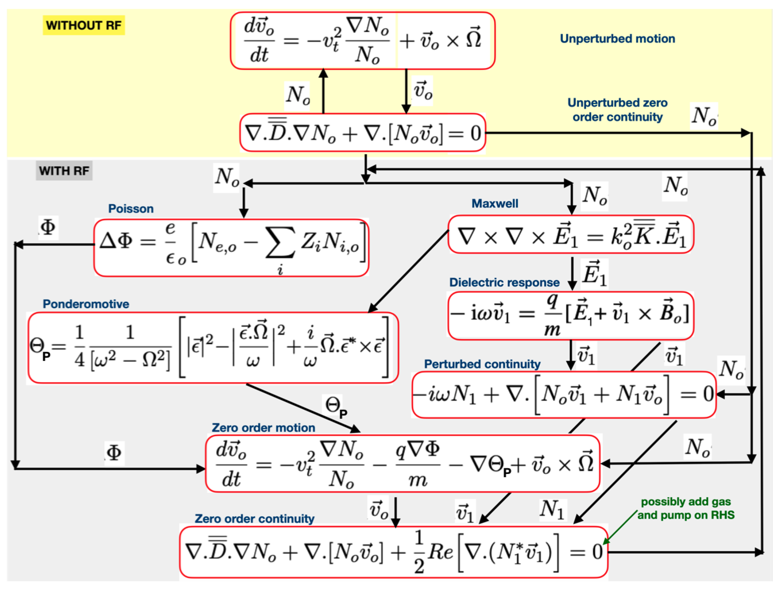
2. Adopted Set of Equations

Figure 1 shows the flow diagram of the logic adopted in this paper. RF waves are launched into the plasma at a given (driver) frequency. Since the contribution of the RF fields to the total Lorentz force is typically small compared to that of the confining magnetic field, the interaction between the charged particles and the waves is commonly described using the quasilinear approach: a set of linear equations describes the dynamics of the perturbed quantities themselves and the net effect of these perturbations after averaging over a driver period yields finite second-order net corrections that add small but non-negligible corrections to the zero-order slow time scale dynamics. The fast RF fields are governed by Maxwell’s equations,

$$\nabla \times \nabla \times {\overrightarrow{E}}_1=k_o^2\stackrel{=}{K}·{\overrightarrow{E}}_1=k_o^2\left(\stackrel{=}{1}+\sum _{\alpha }{\stackrel{=}{K}}_{\alpha }\right)·{\overrightarrow{E}}_1,$$

(1)

where ${\overrightarrow{E}}_1$ is the electric field, $\stackrel{=}{K}$ is the dielectric tensor, ${\stackrel{=}{K}}_{\alpha }$ is the contribution to the tensor by a specie $\alpha$, and $\stackrel{=}{1}$ is the unity matrix. Since the edge temperature is very low, the cold plasma dielectric tensor is suitable:

$${\stackrel{=}{K}}_{\perp 1,\perp 2,//}=\left(\begin{array}{ccc}S& -iD& 0\\ +iD& S& 0\\ 0& 0& P\end{array}\right).$$

(2)

Here, $k_o=\omega /c$ is the vacuum wave number with $\omega =2\pi f$, where f is the (antenna) driver frequency and c is the speed of light, while S, D, and P are the Stix coefficients [22],

$$S=\frac{R+L}{2},$$

$$D=\frac{R-L}{2},$$

$$R=1-\sum _{\alpha }\frac{{\omega }_{p,\alpha }^2}{\omega (\tilde{\omega }+{\mathsf{\Omega }}_{\alpha })},$$

(3)

$$L=1-\sum _{\alpha }\frac{{\omega }_{p,\alpha }^2}{\omega (\tilde{\omega }-{\mathsf{\Omega }}_{\alpha })},$$

$$P=1-\sum _{\alpha }\frac{{\omega }_{p,\alpha }^2}{\omega \tilde{\omega }},$$

where $\tilde{\omega }=\omega +i{\nu }_{\alpha }$ with ${\nu }_{\alpha }$ the collision frequency of the species $\alpha$ being treated. The cold plasma dielectric tensor (2) was obtained solving the perturbed equation of motion for each of the species $\alpha$, providing an explicit expression for the perturbed velocity,

$${\overrightarrow{v}}_{1,\alpha }=-i\omega \frac{q_{\alpha }}{m_{\alpha }}\frac{{\stackrel{=}{K}}_{\alpha }·\overrightarrow{E}}{{\omega }_{p,\alpha }^2}.$$

(4)

The tensor is expressed in terms of a coordinate frame based on the static magnetic field orientation: ${\overrightarrow{e}}_{//}={\overrightarrow{B}}_o/B_o$, ${\overrightarrow{e}}_{\perp ,1}$ is perpendicular to the local magnetic surface ($\rho =\mathrm{const}$ with $\rho$ characterising magnetic surfaces) and ${\overrightarrow{e}}_{\perp ,2}$ lies in the magnetic surface but is perpendicular to the static magnetic field. The plasma and cyclotron frequencies are defined by ${\omega }_{p,\alpha }={\left[\left(N_{\alpha }{q}_{\alpha }^2\right)/\left({ϵ}_o{m}_{\alpha }\right)\right]}^{1/2}$ and ${\mathsf{\Omega }}_{\alpha }=\left(q_{\alpha }{B}_o\right)/m_{\alpha }$, in which $B_o$ is the static magnetic field strength, ${ϵ}_o$ is the vacuum permittivity, $q_{\alpha }$ the charge and $m_{\alpha }$ the mass. $N_{\alpha }$ is the density of species $\alpha$. The geometry is kept extremely simple. Curvature effects are neglected altogether but some of the geometry details need to be retained. We identify the toroidal direction with ${\overrightarrow{e}}_z$. The coordinates x and y are then representing the radial direction (so inside the plasma $x=\mathrm{const}$ defines a magnetic surface $\rho =\mathrm{const}$), while y parametrises the poloidal direction. To account for poloidal field effects and for the fact that the magnetic surfaces nor the antenna are necessarily aligned with the main direction of variation, two angles are introduced. The first angle is the angle between the total magnetic field and the toroidal direction. The second angle is the angle between the equatorial plane of the tokamak and the magnetic surface. The dielectric tensor appearing in the wave equation then is related to the one given above by the double rotation,

$${\stackrel{=}{K}}_{x,y,z}={\stackrel{=}{R}}_2^{-1}·{\stackrel{=}{R}}_1^{-1}·{\stackrel{=}{K}}_{\perp 1,\perp 2,//}·{\stackrel{=}{R}}_1·{\stackrel{=}{R}}_2,$$

(5)

where

$$\left(\begin{array}{c}{E}_{\perp ,1}\\ E_{\perp ,2}\\ E_{//}\end{array}\right)=\left(\begin{array}{ccc}1& 0& 0\\ 0& \cos \mathsf{\Theta }& -\sin \mathsf{\Theta }\\ 0& \sin \mathsf{\Theta }& \cos \mathsf{\Theta }\end{array}\right)·\left(\begin{array}{c}{E}_{\rho }\\ E_{\theta }\\ E_{\phi }\end{array}\right)={\stackrel{=}{R}}_1·\left(\begin{array}{c}{E}_{\rho }\\ E_{\theta }\\ E_{\phi }\end{array}\right),$$

(6)

$$\left(\begin{array}{c}{E}_{\rho }\\ E_{\theta }\\ E_{\phi }\end{array}\right)=\left(\begin{array}{ccc}\cos \theta & \sin \theta & 0\\ -\sin \theta & \cos \theta & 0\\ 0& 0& 1\end{array}\right)·\left(\begin{array}{c}{E}_R\\ E_Z\\ E_{\phi }\end{array}\right)={\stackrel{=}{R}}_2·\left(\begin{array}{c}{E}_R\\ E_Z\\ E_{\phi }\end{array}\right),$$

(7)

with $\theta$ the poloidal angle and $\phi$ the toroidal angle; $(R,Z,\phi )$ is a set of cylindrical coordinates with R a major radius coordinate ($R=0$ being the symmetry axis of the tokamak), and Z the position above or below the equatorial plane (defined by $Z=0$). For what concerns the topic addressed in the present paper, these rotations mainly affect the slow wave behaviour. The former, e.g., allows the slow wave to be directly excited at the antenna even if the wave launcher is purely poloidal (i.e., intended to excite the fast wave). A sketch of the geometry is depicted in Figure 2.

Ideally, no wave energy is staying behind in the edge. To enable modelling of the RF electric field close to the antenna without having to account for the main plasma, one often introduces an artificial damping at all extremities of the integration domain except those close to the launcher to mimic the damping in a well absorbing target plasma. Glancing at how collisionless damping in a hot plasma is accounted for (in its simplest form and for Maxwellian plasmas, the cold plasma resonance is then replaced by the Fried–Conte function which smooths the resonance as far as wave propagation is concerned while introducing a finite imaginary part—mimicking the shape of the distribution function—that describes the damping) and looking at the decoupled fast and slow wave dispersion equation roots, it is suggested that one can add extra damping in the cold plasma equations by merely adding a small but finite imaginary part to the S factor of Stix—which allows to boost the fast wave damping—while doing the same on the P factor—which manages the same artificial damping for the slow wave. These corrective modifications are only added close to the left and top+bottom edges (a Gaussian shape was used); when purely outgoing waves are described, the strength and width are adjusted to ensure the wave is fully damped before reaching the actual edge of the integration domain while also leaving the near-field region untouched. The mean effect of the RF field gives rise to a finite ponderomotive potential. In absence of the magnetic field this potential is simply related to the gradient of the amplitude squared of the electric field [23] but in presence of a dominant static magnetic field its expression is somewhat more involved. The ponderomotive acceleration for each of the charged species is then of the form ${\overrightarrow{a}}_{\mathrm{pond}}=-\nabla \mathsf{\Theta }{}_P$, where [21]

$$\begin{array}{ccc}\hfill \mathsf{\Theta }{}_P& =& \frac{1}{4}\frac{1}{\left({\omega }^2-{\mathsf{\Omega }}^2\right)}\left[|\overrightarrow{ϵ}{|}^2-{\left|\frac{\overrightarrow{ϵ}·\overrightarrow{\mathsf{\Omega }}}{\omega }\right|}^2+\frac{i}{\omega }\overrightarrow{\mathsf{\Omega }}·{\overrightarrow{ϵ}}^{*}\times \overrightarrow{ϵ}\right]\hfill \end{array}$$

(8)

where $\overrightarrow{\mathsf{\Omega }}=q{\overrightarrow{B}}_o/m$ and $\overrightarrow{ϵ}=q{\overrightarrow{E}}_1/m$. In the RF domain, the electron cyclotron frequency is much larger than the driver frequency so that the dominant electric field component for the electrons is $E_{//}$. For the ions, on the other hand, the driver frequency and the cyclotron frequency are of the same order so that it is the perpendicular components that matter mostly. Note also that the ion ponderomotive potential can be further boosted when the driver frequency is close to the cyclotron frequency of the ion species. For obvious reasons, one avoids cyclotron layers (and thus cyclotron damping) to be present in the edge, however.

An electrostatic potential, $\mathsf{\Phi }$, arising from slow time scale violation of charge neutrality is prescribed by the Poisson’s equation,

$$\Delta \mathsf{\Phi }={\frac{e}{ϵ}}_o\left(N_{e,o}-\sum _i{Z}_i{N}_{i,o}\right),$$

(9)

where $N_{e,o}$ and $N_{i,o}$ are the zero-order electron and ion densities.

While the fast time scale motion is known analytically and gives rise to the cold plasma dielectric tensor, the slow time scale equation of motion needs to be evaluated for each of the species individually. Aside from the dominant Larmor gyration term and the term arising from the pressure it contains the slow time scale effects of the presence of the RF fields (the ponderomotive potential $\mathsf{\Theta }{}_P$) and of the charge separation indirectly resulting from the presence of the RF fields (the electrostatic potential $\mathsf{\Phi }$) [21]:

$$\frac{d{\overrightarrow{v}}_o}{dt}=-v_t^2\frac{\nabla N_o}{N_o}-\frac{q\nabla \mathsf{\Phi }}{m}-\nabla {\mathsf{\Theta }}_P+{\overrightarrow{v}}_o\times \overrightarrow{\mathsf{\Omega }}.$$

(10)

Here, the vector $\overrightarrow{\mathsf{\Omega }}$ is along the magnetic field and its magnitude is the cyclotron frequency, and $v_t={(kT/m)}^{1/2}$ is the thermal velocity. It was implicitly assumed that the temperature $T=T_e=T_i$ is constant so that it can be moved out of the gradient; k is the Boltzman constant. The electrostatic field corresponding to the potential arising from charge neutrality breaking is ${\overrightarrow{E}}_o=-\nabla \mathsf{\Phi }$. Note that this is a non-linear equation since $d{\overrightarrow{v}}_o/dt=\partial /\partial t+{\overrightarrow{v}}_o·\nabla {\overrightarrow{v}}_o$. Assuming a quasi-steady state exists ($\partial /\partial t=\nu$, where $\nu$ is the collision frequency for the species treated), the above equation reduces to

$$-{\overrightarrow{v}}_o·\nabla {\overrightarrow{v}}_o+{\overrightarrow{v}}_o\times \overrightarrow{\mathsf{\Omega }}-\nu {\overrightarrow{v}}_o=v_t^2\frac{\nabla N_o}{N_o}+\frac{q\nabla \mathsf{\Phi }}{m}+\nabla {\mathsf{\Theta }}_P=\overrightarrow{R}.$$

(11)

The collision frequency was added to account for collisional damping of the motion and to be fully consistent with the adopted dielectric tensor. In the context of the present study the sole role of this relatively small collisional contribution is to bend resonances into quasi-resonances allowing to avoid the need for analytical matching across resonances by adopting a sufficiently refined grid but without affecting the power balance. When omitting the non-linear term, the equation of motion can actually be solved analytically:

$$v_{ox}=\frac{-\left(\nu R_x+\mathsf{\Omega }{R}_y\right)}{{\mathsf{\Omega }}^2+{\nu }^2},v_{oy}=\frac{-\nu R_y+\mathsf{\Omega }{R}_x}{{\mathsf{\Omega }}^2+{\nu }^2}.$$

(12)

In absence of the perturbations caused by the RF field, the density in front of the antenna is dominantly depending on the radial coordinate (x in the rotated local Cartesian grid) so the dominant velocity is a uniform drift along the antenna strap. The corresponding velocity shear being in the radial direction makes that $\nabla ·{\overrightarrow{v}}_o\approx 0$ and ${\overrightarrow{v}}_o·\nabla {\overrightarrow{v}}_o\approx \overrightarrow{0}$. Non-linear corrections can arise when RF corrections are added but, the RF field being a perturbation, they can usually be neglected. Knowing the velocities, one can solve the fast and slow time scale densities for each of the species leaning on the continuity equation. Following the same (quasilinear) logic as before and writing the continuity equation into a zero-order, a first-order and second-order contribution, the fast time scale (first-order) density is

$$-i\omega N_1+\nabla ·\left(N_o{\overrightarrow{v}}_1+N_1{\overrightarrow{v}}_o\right)=0.$$

(13)

Assuming a steady state can be reached the zero-order density satisfies

$$\nabla ·\stackrel{=}{D}·\nabla N_o+\nabla ·\left(N_o{\overrightarrow{v}}_o\right)+\frac{1}{2}\mathrm{Re}\left[\nabla ·\left(N_1^{*}{\overrightarrow{v}}_1\right)\right]=0,$$

(14)

to which a diffusion matrix allowing both for radial and (depending on the rotation angle of the ${\overrightarrow{B}}_o$ field) poloidal or partially-parallel diffusion was added since mobility along and across magnetic surfaces is a key player to set up the density profile. This is a mock-up to qualitatively attempt to describe the much bigger excursions particles make due to their temperature than what fluid velocities indicate: a 10 eV D ion already has a thermal speed of 22 km/s. Note that the last term in the above is a quasilinear correction due to the net finite effect of the presence of the RF field. The latter equation closes the loop: the electromagnetic and electrostatic response to the new densities can be used to define an update of the fields and potentials.

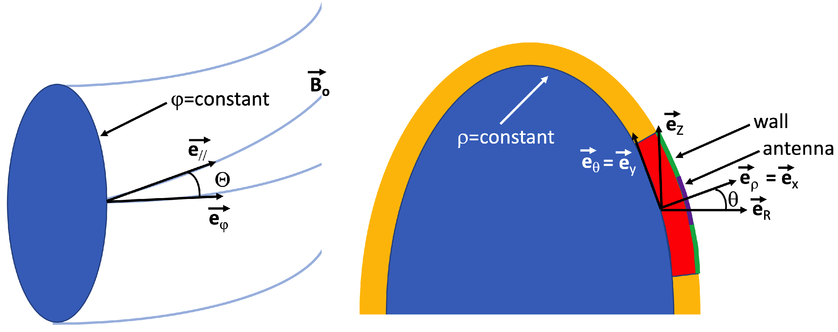
3. Boundary Conditions

The adopted geometry is as follows: the antenna is assumed to be situated on the right and the main plasma on the left extremes of the integration interval. As the y-direction is representing the (unfolded) poloidal direction, two logical options are: (i) to assume the full poloidal circumference is being modeled so that the top and bottom values values are identical (in as far as enough degrees of freedom are available), and (ii) to assume the field lines hit a metallic object. The former of these choices models the case of actual magnetic surfaces, while the latter are more relevant for field lines intersecting a septum and are more relevant when describing sheath effects, a topic left for later work.

The adopted boundary conditions for the various equations are:

• For the rapidly varying electric field (Maxwell’s equations for waves in cold plasma):

  –

  4th-order equation, so four boundary conditions in each direction,

  –

  $E_y$ imposed and $E_z=0$ at antenna side,

  –

  purely outgoing wave or metallic boundary conditions at the plasma edge (but—if desired—artificial damping imposed to ensure waves are damped before actually reaching the edge),

  –

  $E_y$ and $E_z$ and their poloidal derivatives identical at top and bottom.

• For the electrostatic potential (Poisson’s equation modelling the effect of charge neutrality breaking):

  –

  2nd-order equation, so one boundary condition at each edge,

  –

  at the plasma side, force the potential to be zero: no RF perturbations far away from the antenna,

  –

  at the antenna side and since the antenna is a metallic object, either impose a zero normal derivative (electric field perpendicular to metallic object) or impose a potential (imposed by the loading of the metallic wall when field lines not fully parallel to it),

  –

  on the poloidal side impose the potential and its normal derivative to be identical on top and bottom.

• For the slowly varying density ($N_o$ continuity equation):

  –

  2nd-order equation, so one boundary condition at each side,

  –

  impose $N_o$ to be identical to the imposed one at the plasma side: no perturbation far away from the wave launcher,

  –

  impose negligible density at the antenna side (except for small corrections, exponential decay beyond the last closed flux surface),

  –

  impose same $N_o$ and normal derivative at top and bottom (poloidal) side.

• For the fast-varying density ($N_1$ continuity equation):

  –

  1st-order equation, so one boundary condition only on one side in each direction,

  –

  no perturbation at plasma side well away from antenna,

  –

  same density top/bottom.

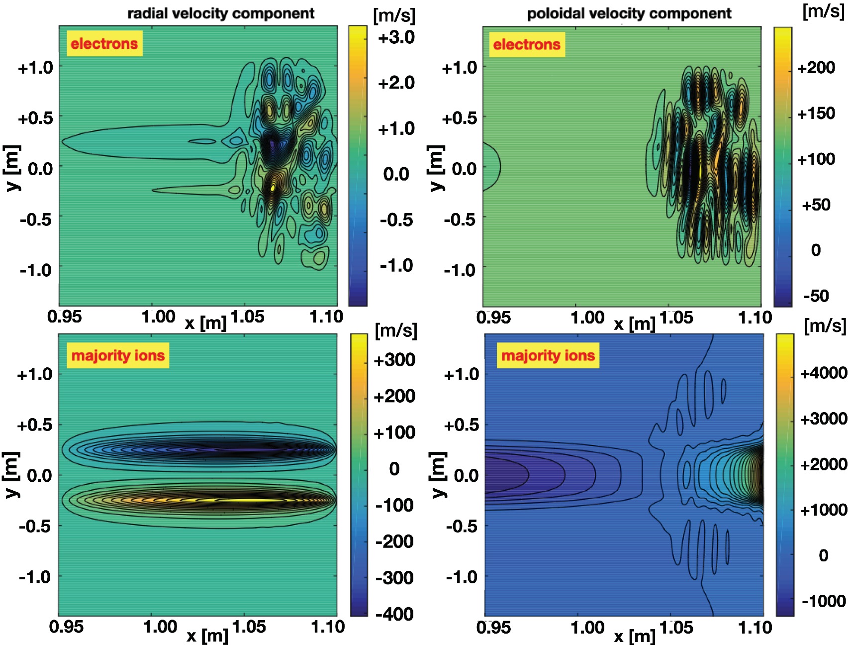
• For the slowly varying velocity for each of the species (equation of motion):

  –

  check if the non-linear term is significant; if not, simply omit it and solve this equation analytically,

  –

  if the term is required: transform the non-linear equation into a series of linear “adiabatic switch-on” artificial time steps with the non-linear solution as the asymptotic solution of the linearized problem,

  –

  1st-order vector equation, so one boundary for each unknown only on one side,

  –

  ${\overrightarrow{v}}_o=\overrightarrow{0}$ at plasma side: no RF-induced perturbation far away from the RF launcher,

  –

  same velocity top and bottom.

4. General Purpose Solver

Equation and Boundary Conditions

As we have at most second-order derivatives we build a generic partial differential equation solver for equations of the general type:

$${\stackrel{=}{A}}_{xx}·\frac{{\partial }^2}{\partial x^2}\overrightarrow{Y}+{\stackrel{=}{A}}_{xy}·\frac{{\partial }^2}{\partial x\partial y}\overrightarrow{Y}+{\stackrel{=}{A}}_{yy}·\frac{{\partial }^2}{\partial y^2}\overrightarrow{Y}+{\stackrel{=}{A}}_{0x}·\frac{\partial }{\partial x}\overrightarrow{Y}+{\stackrel{=}{A}}_{0y}·\frac{\partial }{\partial y}\overrightarrow{Y}+{\stackrel{=}{A}}_{00}·\overrightarrow{Y}=\overrightarrow{0}$$

(15)

with a set of boundary conditions of the general type,

$$\sum _{j=1}^{N_F}{B}_{x,\alpha ,i,j}\frac{\partial }{\partial x}{Y}_j+B_{y,\alpha ,i,j}\frac{\partial }{\partial y}{Y}_j+B_{0,\alpha ,i,j}{Y}_j=S_i,$$

(16)

at each of the four walls designated via the $\alpha$. All equations are solved using the same solver by merely properly defining the relevant coefficients and reading them into the solver. The $\stackrel{=}{A}$ matrices have dimensions $(N_{eq},N_F)$, where $N_{eq}$ is the number of equations and $N_F$ is the number of unknowns to be determined. The index j scans over all unknowns while the index i scans over all boundary conditions for a given side $\alpha$. The above boundary conditions allow to impose local boundary conditions. For the purposes of the present study, this is not sufficient: to be able to impose variables and their derivatives to be identical at opposite sides of the integration interval we need to extend the generic boundary condition to

$$\sum _{\alpha =1}^4\sum _{j=1}^{N_F}{B}_{x,\alpha ,i,j}\frac{\partial }{\partial x}{Y}_j+B_{y,\alpha ,i,j}\frac{\partial }{\partial y}{Y}_j+B_{0,\alpha ,i,j}{Y}_j=S_i,$$

(17)

where the sum is on the alphas on opposite sides of the integration interval (points with one common coordinate and first and last point in the remaining coordinate). The boundary conditions are imposed using Lagrange multipliers, which allows to impose the reigning equation at all points, including those at which the boundary conditions are imposed. Additionally, several boundary conditions can in principle be imposed at corner points. The resulting system of linear equations is solved by standard sparse matrix inversion techniques adopting the MUMPS solver [24].

5. Examples

The present section illustrates the type of solutions the various equations provide and culminates in putting the various pieces of the puzzle together, solving the series of equations in a closed loop. The parameters are loosely inspired on those of the JET tokamak. A major radius of $R_o=2.96$ m and a minor radius of $a_p=0.95$ m was assumed. A deuterium plasma is considered. The RF frequency is 51 MHz which allows for central hydrogen and deuterium heating when considering the static magnetic field to be $B_o=3.45$ T at the magnetic axis. It was assumed that the magnetic field is tilted by $\mathsf{\Theta }=0.2$ rad with regards to the toroidal direction. The antenna is assumed to be symmetrical with respect to the equatorial plane so that $\theta =0$. In the wave equation the collision frequency allows to turn resonances into quasi-resonances at which resonant absorption occurs but its actual value is immaterial as long as it is sufficiently small. Dipole phasing of JET’s A2 antenna has a dominant $k_{//}$ of about 6/m. When evaluating the ponderomotive potential, it will—unless otherwise specified—be assumed that 5 MW of power is launched. The antenna’s poloidal length is 50 cm, positioned symmetrically with regards to the equatorial plane $y=0$. A 15 cm radial plasma slice is considered, starting at the last closed flux surface. In the poloidal direction, the integration domain has been limited to just $1.4$ m up and below the equatorial plane to reduce the number of grid points required but the top end is imposed to be identical to the bottom end to simulate the poloidal periodicity.

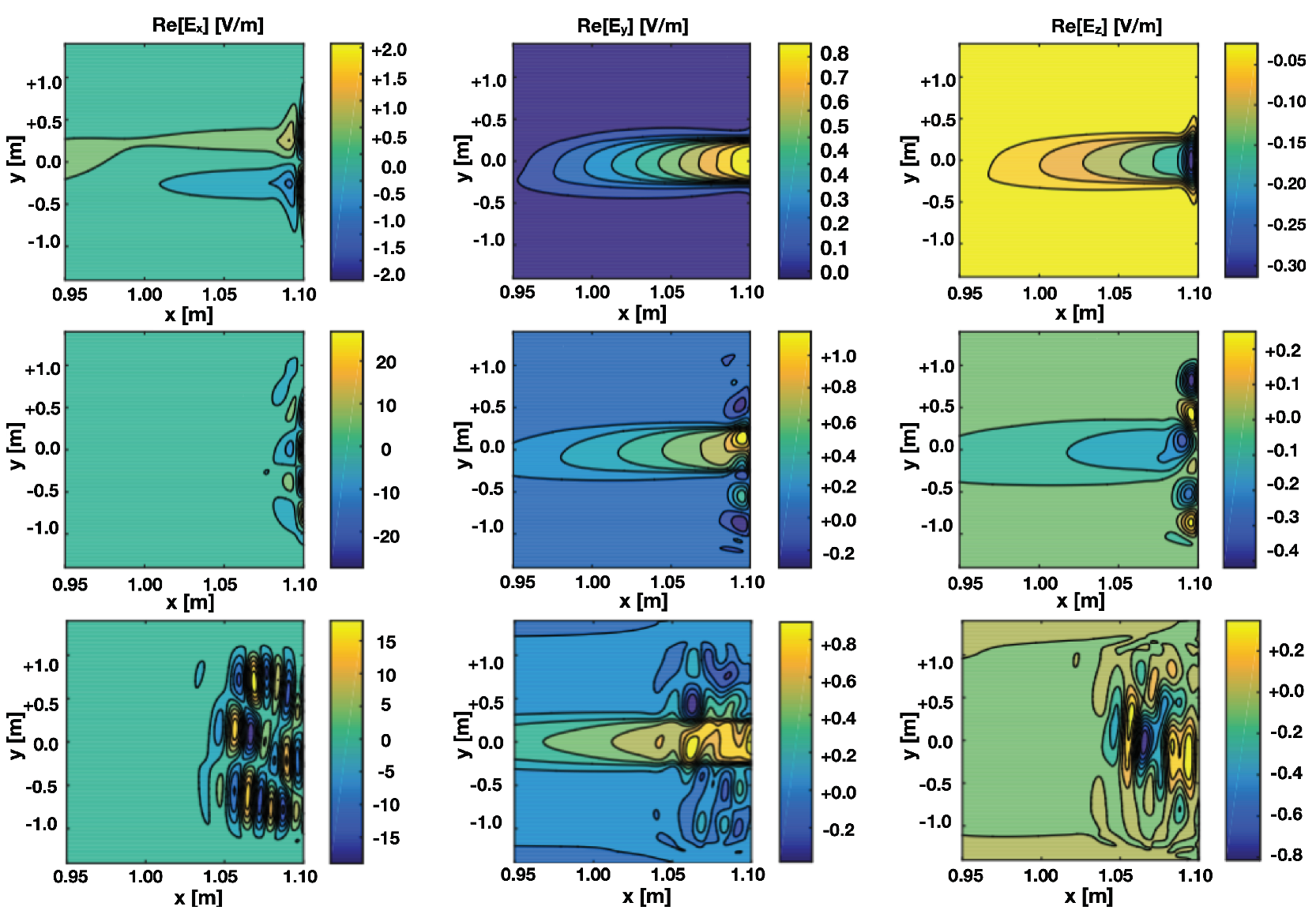
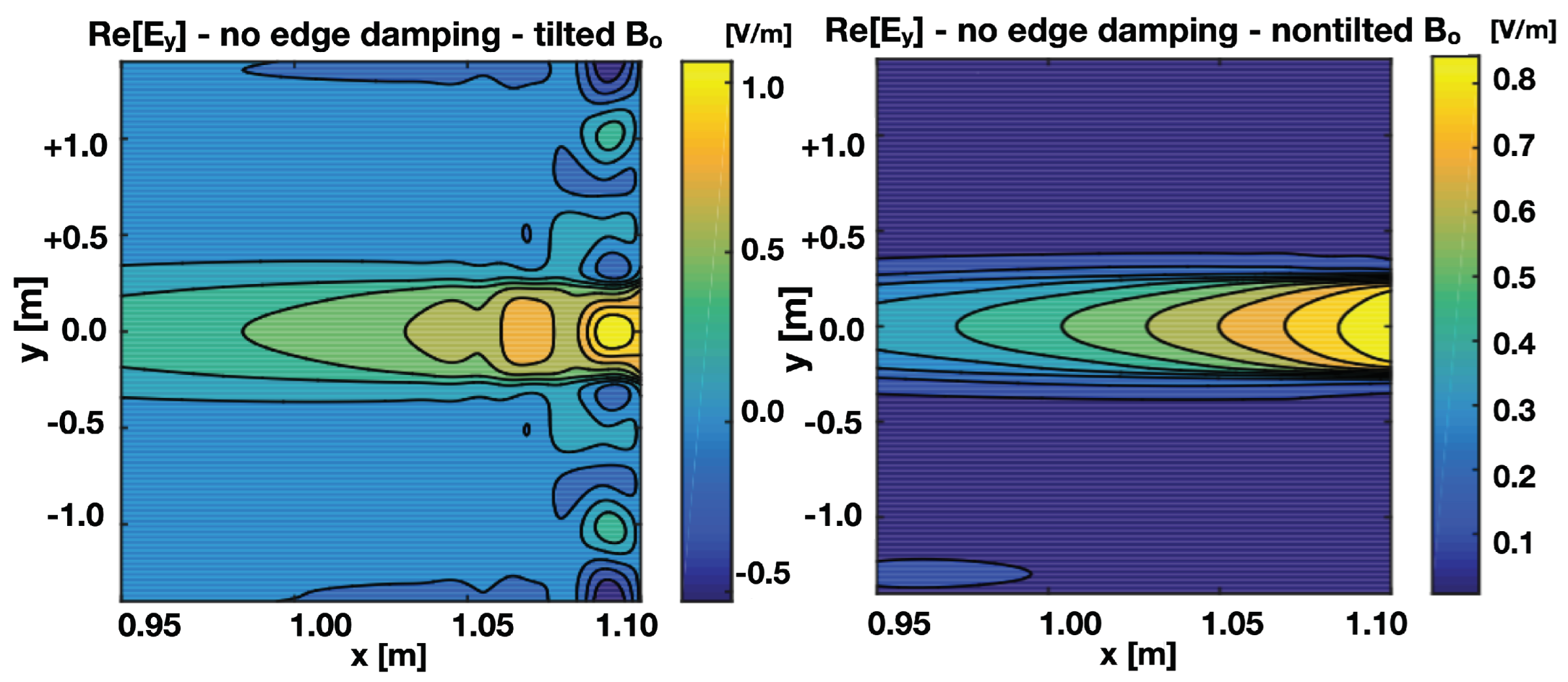
5.1. Solution of the Wave Equation

Figure 3 depicts an example of the electric field for three different densities at the last closed flux surface and assuming an exponential decay length of 3 cm in the scrape-off layer while imposing a unity poloidal electric field ($E_y$ = 1 V/m) at the antenna location. A decay in the shape of an arctangent with a characteristic length of 3 cm was imposed at either antenna end to simulate the gradual electric field drop beyond the end of the launcher strap. Since the magnetic field lines are tilted, the fast wave antenna parasitically partly excites the slow wave. The exponentially evanescent fast wave poloidal field component ($E_{\theta }=E_y$) is well seen in the top middle plot. Slow wave structure is well observed on the real part of the x (radial) component of the field: the slow wave is directly exited at the antenna due to the finite angle between the parallel and the toroidal direction but since the wave is evanescent it only appears close to the launcher for the highest imposed density. It invades gradually more of the plasma when the edge density is decreased (middle and bottom rows plots). Since a unity ”antenna” $E_y$ field amplitude was imposed, these examples do not correspond to the same power launched. Moreover the imaginary part’s contribution to the field amplitude (locally contributing differently for fast and slow waves) has not been depicted. This gives the deceiving impression that the fast wave penetrates better at lower than at higher densities, which is not the case. The wave equation being linear, the amplitude is adapted when imposing a prescribed launched power (as is well seen in Figure 9 below).

In Figure 3, the electric field is artificially damped by adding a finite imaginary part to S and P when approaching the poloidal edge. To better illustrate this case, the poloidal field component in absence of the artificial poloidal edge damping is also shown (Figure 4, left) for the lowest edge density, ${10}^{18}$/m${}^3$. The wave structure close to the right edge is now dominated by the slow wave structure all along the edge. The latter example illustrates that isolating the antenna region from the rest of the machine—as is frequently done when designing antenna’s, implicitly assuming waves never return to the launcher—is not necessarily providing a physically meaningful result: the impact of constructive/destructive interference in the region, where waves are admitted but are not fully or are only weakly damped, is artificially suppressed by such a procedure. Whether the slow wave plays an active role or not depends on the efficiency with which it is excited, either directly at the antenna—as is the case in the latter example—or at its confluence near the ion–ion hybrid layer with the fast wave. To capture the mode a sufficiently fine grid needs to be adopted: a grid coarser than the slow wave characteristic length artificially screens the wave and gives the wrong impression it does not play a role. However, in many cases the distance between the ion–ion hybrid layer (where the slow wave is excited by the fast wave) and the lower hybrid layer (where it is absorbed) is small and the slow wave does not take front stage. Additionally, towards the main plasma—where significant damping is present when properly tuning the frequency to the magnetic field—assuming purely outgoing waves from the antenna region is a poor representation if single pass absorption is not guaranteed so that waves need to wash over the main plasma multiple times before being fully absorbed. Figure 4, right, depicts the poloidal electric field component when the toroidal and parallel directions coincide. The shorter wave structure has now disappeared. Recall that we imposed the poloidal and toroidal electric field, as well as their poloidal derivatives to be identical at the top and bottom of the integration interval.

When the electric field pattern consistent with a prescribed excitation on the antenna has been obtained, the ponderomotive potential, $\mathsf{\Theta }{}_P$, can be evaluated. First, the total flux Poynting emanating from the antenna is evaluated. Next, the electric field magnitude is rescaled to an assumed launched power. The acceleration corresponding to the ponderomotive potential involves the gradient of the potential. The acceleration is not in the direction of the gradient—as is the case in absence of the confining magnetic field $B_o$—but is perpendicular to it. Provided a steady state is reached and assuming the non-linear term is not of significance, the resulting velocity when solving the equation of motion is perpendicular both to the field and to the force. An example is shown in Figure 5. Note that the image is consistent with the notion of “convective cells” brought about by the RF field: first look at the bottom plots representative for the ions and the fast wave. At either end of the antenna strap, the radial velocity is significant, as shown in Figure 5, left. At the bottom, the velocity points towards the antenna while, at the top, it points away from it. Figure 5, right, shows upward (poloidal) movement along the antenna blade and downward motion well away from the launcher. The total motion is that of a convective cell, pulling particles towards the antenna at the bottom of the strap, forcing them to stream upwards along the antenna, pushing them away at the top of the strap and closing the “cell” away from the antenna. This image is somewhat deceptive, though. The velocities in the radial and poloidal directions are not similar in magnitude, so that the dominant effect is the creation of an up–down asymmetry. Looking at the top plots one sees a similar picture but since the electrons are more vulnerable to effects caused by the parallel electric field, they form convective cells imposed by the slow wave rather than by the fast wave structure. As a consequence the cells are smaller in magnitude. This kind of streaming was already illustrated in Ref. [25], see Figures 3–5 there. In this earlier study, the description was not fully self-consistent, however. The aim of the present paper is to remove that drawback. The idea of convective cells indirectly driven by RF electric fields goes back to even older notions, however; see, e.g., [26]. In the latter, the inward and outward flux was already attributed to the simultaneous presence of a strong confining magnetic field and a DC (direct current) electric field arising from the presence of RF fields. What is added now is the notion that this happens under the influence of ponderomotive effects, and that the inward and outward push is mainly at the antenna tips if fast wave physics is important while it can occur close or far away from the antenna if the slow wave imposes the motion.

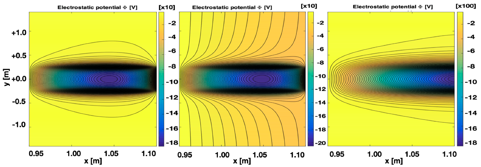
5.2. Poisson’s Equation

Charge neutrality breaking gives rise to a nonzero electrostatic potential being created. It is commonly assumed that electrons are mobile because of their small mass and can compensate imbalances quickly. In the presence of a strong confining magnetic field, rapid balancing perpendicular to magnetic field lines is strongly hindered, however, while flow along the field lines is not. If the magnetic field lines intersect metallic objects, the wall material tends to load up negatively in view of the high mobility of the electrons. In this Subsection, an artificial Gaussian charge separation with a characteristic width of 3 cm is imposed at the antenna while neutrality is achieved elsewhere. Prior to actually closing the loop and solving all equations in a cycle, this is done to acquire a feeling of the magnitude of voltages required to compensate mild charge separation breaking. Violating the charge neutrality by density differences as tiny as ${10}^{14}$/m${}^3$ (i.e., 5–6 orders of magnitude smaller than the densities in the main plasma) in the considered 15 cm narrow interval between the last closed flux surface and the antenna requires potentials to have values in the 10kV range: neglecting the poloidal (y) dependence so just retaining the radial (x) variation when estimating the ballpark magnitude of the potential and assuming the potential, as well as its derivative, are zero at the plasma side ($x=x_{\mathrm{ref}}=0.95$ m), while the charge neutrality breaking is the same throughout the domain, the solution of $d^2\mathsf{\Phi }/d{x}^2=C$ is $\mathsf{\Phi }=C{(x-x_{\mathrm{ref}})}^2/2$, where $C=e/{ϵ}_o·{10}^{14}/{\mathrm{m}}^3$, so that $\mathsf{\Phi }$ would reach about 20 kV. Smaller regions, where charge neutrality is broken, reduce these high voltages: under the same boundary condition, $d^2\mathsf{\Phi }/d{x}^2=0$ (charge neutrality in the whole domain), yields $\mathsf{\Phi }=0$, while dropping down the region of charge neutrality breaking to 1 cm would yield $\mathsf{\Phi }=90$ V. Solutions of the Poisson’s equation with the Gaussian source are depicted in Figure 6. Closer to the antenna, where the charge neutrality is broken, the slope of the potential is imposed by the Gaussian and the requirement to satisfy the boundary condition at the antenna side. Higher slopes allow more modest voltages and shallower slopes require higher ones. In Figure 6, left, it is assumed that the potential at the antenna is zero, while in Figure 6, middle, it is assumed the antenna charges up to a static potential of −35 V; in Figure 6, right, it is assumed that the normal derivative vanishes at the antenna. The antenna being a metallic object, this condition seems the more logical one to be used. It requires voltages to raise to about $1.8$ kV. In the other two examples of Figure 6, the voltages remain quite modest but the gradients are much steeper, so the corresponding electric field is significant as well. The obtained results show that even modest enough charge neutrality breaking gives rise to significant restoring electrostatic fields.

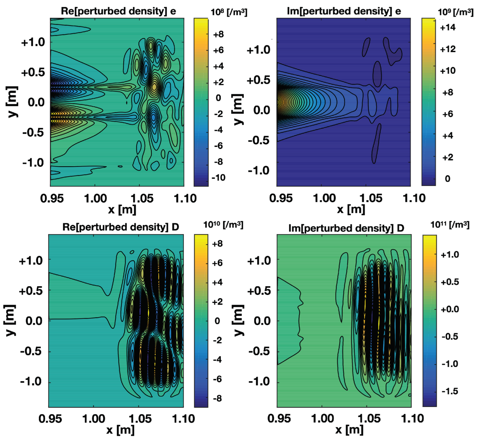
5.3. Perturbed Density

The perturbed density is computed solving the continuity equation for the perturbed quantities. It represents a relatively small correction to the main plasma density but it is not necessarily negligible in the region close enough to the antenna, where other effects than those reigning the confined plasma determine the density response. Figure 7 provides an example showing the electron density perturbation is smaller than that of ions. From Equations (1)–(4), one can see that the perturbed electron motion is present dominantly in the parallel direction, while that of ions present mainly in the perpendicular direction. Since the product of the density and velocity (see Equation (14)) will constitute the “source” term for the zero-order density, it is expected the RF induced electron corrections to the zero-order density in the radial direction will be less pronounced.

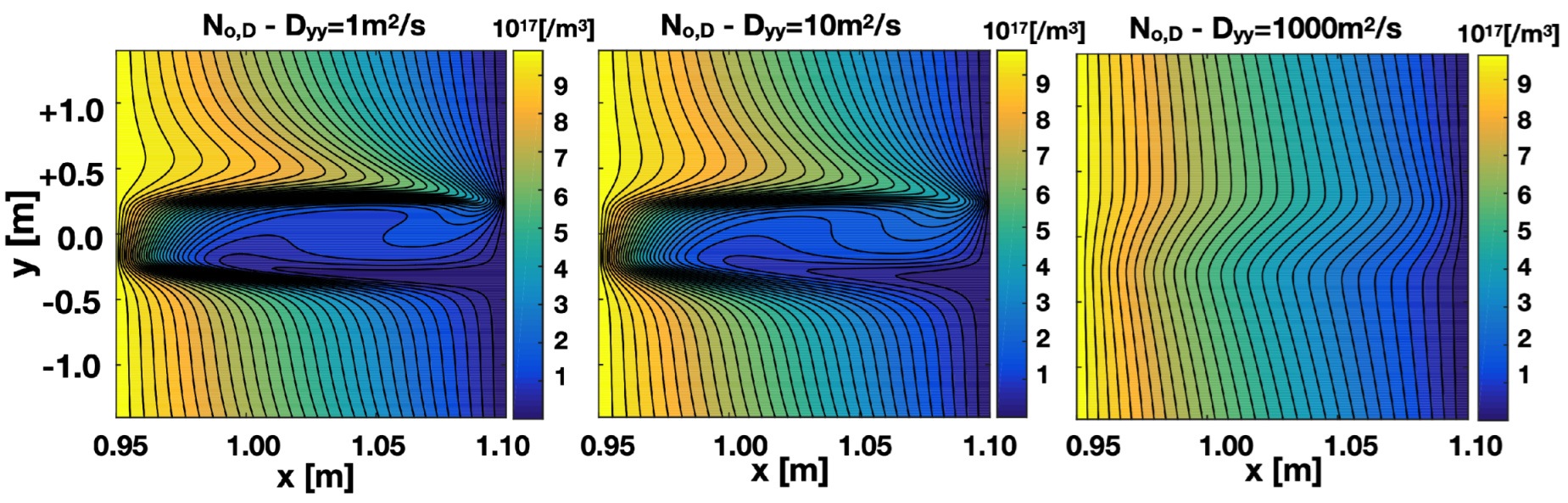
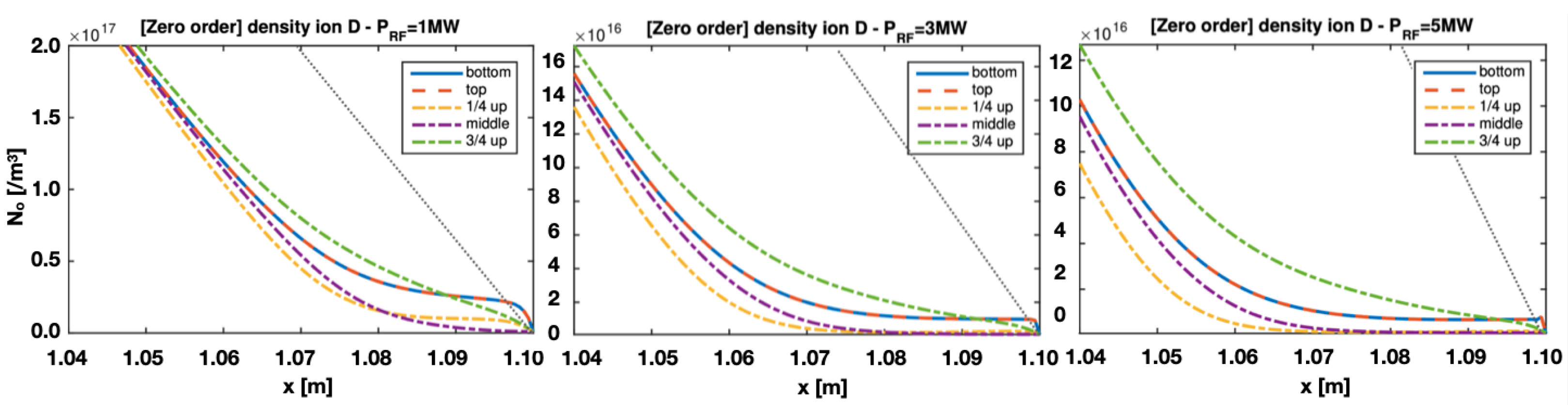
5.4. Zero-Order Density Correction

Aside from the zero-order velocities, which have been evaluated solving the equation of motion, and the quasilinear correction term, which appears in the right-hand side of the zero-order continuity equation used to find the zero-order density, knowledge of the diffusion strength parallel and perpendicular to magnetic surfaces is required. Aligned with values consistent with neoclassical theory, the diffusion across field lines is assumed to be $D_{xx}=1$ m${}^2$/s. Since the mobility along the magnetic field lines is much higher than that across them, the parallel diffusion will accordingly be assumed to be much higher. Figure 8 depicts the zero-order density for three parallel diffusion strengths: one at very low ($D_{yy}=1$ m${}^2$/s; Figure 8, left), one at low ($D_{yy}=10$ m${}^2$/s; Figure 8, middle), and one at moderately high ($D_{yy}=1000$ m${}^2$/s; Figure 8, right) levels. As expected, the impact of the diffusion is to smear out the particles. The higher the parallel diffusion, the more uniform the density becomes in the parallel direction.

One can also conclude that the single-most important equation in the set of Equations (1), (4), and (8)–(14) solved iteratively, as depicted in Figure 1, is the Poisson’s Equation (9) modelling the breaking of the charge neutrality. Ensuring an as accurate as possible model for the density corrections in the right-hand side of that equation is key since very modest deviations from charge neutrality already give rise to significant overall changes.

Upon several iterations, one finds that the non-linear term in the equation of motion is negligible. Hence, adopting the analytical expression of the velocity rather than actually solving the partial differential equation of motion is permissible and allows us speeding up the numerical procedure.

Figure 9 represents the main result of the present paper and depicts the zero-order density for different RF powers launched when solving the set of equations and looping to account for adjustments of electric field patterns caused by changes in the densities, as well as to account for modifications of the densities resulting from the computed electric fields: three different power levels have been adopted, namely $P_{\mathrm{RF}}=1$ MW (Figure 9, left), $P_{\mathrm{RF}}=3$ MW (Figure 9, middle), and $P_{\mathrm{RF}}=5$ MW (Figure 9, right). The impact of the presence of the RF field is that the density is strongly reduced in front of the antenna but—because of the strong diffusion along the magnetic field lines and because of the asymmetry imposed by the ponderomotive effects—also poloidally away from it. The part of the densities where it is linear and attaches to the imposed density at the last closed flux surface (${10}^{18}$/m${}^3$) is not shown but the density in absence of the RF waves is equally drawn (dotted grey line) to provide an idea of the magnitude of the density change.

An important side remark needs to be made at this point. Although the effect of the presence of the RF field on the density confirms experimental findings, a key aspect of the physics has been side-stepped: close to metallic objects and because of the essentially different mobility of ions and electrons for similar temperatures, sheaths tend to form. These correspond to fierce charge neutrality breaking on the scale of the Debye length, a scale much shorter than the grid spacing adopted in the present paper. For that reason, the results obtained here most certainly need to be scrutinised further to better account for the impact of sheaths. Parallel expulsion along the field lines was not even discussed, although it is of importance, as the simple model invoking diffusion to crudely represent the different parallel and perpendicular mobility already testifies in an ad hoc way when admitting a field line tilt. A more rigorous treatment of the fluid theory of ponderomotive forces in presence of a strong magnetic field than Klima’s was later provided by Lee and Parks [27]. Ref. [27] underlines that Klima [21] adopts two-fluid cold plasma expressions to compute the time averaged forces. Ref. [27] states that the model exploited in the present paper when compared to the more complete findings of Ref. [27] is approximately the same up to first derivatives but that potentially important (e.g., density) gradient terms are omitted because of the approximation made. Additionally, other authors contributed to further progress (see, e.g., [28,29]). Much more recently, extra efforts—exploiting sophisticated antenna modelling—have been made, e.g., in Refs. [30,31,32,33,34]. The provided examples equally illustrate that the results found sensitively depend on the parameters (e.g., the value of the diffusion coefficients) chosen. A too simple model—ignoring the details of the ionisation and recombination occurring in the edge, as well as the details of the actual plasma–wall interaction (e.g. due to sputtering) —is unlikely to provide more than a qualitative picture of the reigning dynamics. Hence, the present study can—at best—only be considered as a step along the way towards a more rigorous understanding.

6. Conclusions

A simple set of equations was adopted to study the impact of the RF waves on the density in the plasma edge. It is found that the density in front of a radio frequency antenna is affected by the presence of the launched electromagnetic waves: the plasma is pushed away from the antenna and a density asymmetry along the strap is created. Both effects are gradually more pronounced when the launched power is bigger.

References

1. Mailloux, J.; Abid, N.; Abraham, K.; Abreu, P.; Adabonyan, O.; Adrich, P.; Afanasev, V.; Afzal, M.; Ahlgren, T.; Aho-Mantila, L.; et al. Overview of JET results for optimising ITER operation. Nucl. Fusion 2022, 62, 042026. [Google Scholar] [CrossRef]
2. Garzotti, L. Overview of results of scenario development for high fusion performance from DTE2 campaign at JET. In Proceedings of the 48th Annual Plasma Physics Conference, Liverpool, UK, 11–14 April 2022. [Google Scholar]
3. Maggi, C.; JET contributors. Tritium experiments in JET-ILW in support of JET and ITER D-T plasmas. In Proceedings of the 48th EPS Conference on Plasma Physics, online, 27 June–1 July 2022; Available online (abstract): https://indico.fusenet.eu/event/28/contributions/216/ (accessed on 17 December 2022).
4. Challis, C.; Hobirk, J.; Kappatou, A.; Lerche1, E.; Auriemma, F.; Belonohy, E.; Casson, F.J.; Coffey, I.; Eriksson, J.; Field, A.R.; et al. JET contributors. Development of hybrid (high beta) plasmas for deuterium-tritium operation in JET. In Proceedings of the 48th EPS Conference on Plasma Physics, online, 27 June–1 July 2022; Available online: https://indico.fusenet.eu/event/28/contributions/219/ (accessed on 17 December 2022).
5. Maslov, M.; Lerche, E.; Challis, C.D.; Hobirk, J.; Kappatou, A.; King, D.B.; Keeling, D.; Rimini, F.; De La Luna, E.; Monakhov, I.; et al. T-rich scenario for the record fusion energy plasma in JET DT. In Proceedings of the 64th] Annual Meeting of the APS Division of Plasma Physics (APS), Spokane, WA, USA, 17–21 October 2022; Available online (abstract): https://meetings.aps.org/Meeting/DPP22/Session/BI01.3 (accessed on 17 December 2022).
6. Noterdaeme, J.M.; Eriksson, L.-G.; Mantsinen, M.; Mayoral, M.-L.; Eester, D.V.; Mailloux, J.; Gormezano, C.; Jones, T.T.C. Physics studies with the additional heating systems in JET. Fusion Sci. Technol. 2008, 53, 1103–1151. [Google Scholar] [CrossRef]
7. Koch, R. Plasma Heating by neutral beam injection. Fusion Sci. Technol. 2004, 45, 183–192. [Google Scholar] [CrossRef]
8. Messiaen, A.; Maquet, V. Coaxial and surface mode excitation by an ICRF antenna in large machines like DEMO and ITER. Nucl. Fusion 2020, 60, 076014. [Google Scholar] [CrossRef]
9. Maquet, V.; Druart, A.; Messiaen, A. Analytical edge power loss at the lower hybrid resonance: ANTITER IV validation and application to ion cyclotron resonance heating systems. J. Plasma Phys. 2021, 87, 905870617. [Google Scholar] [CrossRef]
10. Giroud, C.; Pitts, R.A.; Kaveeva, E.; Rozhansky, V.; Brezinsek, S.; Huber, A.; Mailloux, J.; Marin, M.; Tomes, M.; Veselova, I.; et al. JET contributors. High performance Ne-seeded baseline scenario in JET-ILW in support of ITER. In Proceedings of the 48th EPS Conference on Plasma Physics, Maastricht, The Netherlands, 27 June–1 July 2022; Available online (abstract): https://indico.fusenet.eu/event/28/contributions/500/ (accessed on 17 December 2022).
11. Colas, L.; Urbanczyk, G.; Goniche, M.; Hillairet, J.; Bernard, J.M.; Bourdelle, C.; Fedorczak, N.; Guillemaut, C.; Helou, W.; Bobkov, V.V.; et al. The geometry of the ICRF-induced wave-SOL interaction. A multi-machine experimental review in view of the ITER operation. Nucl. Fusion 2022, 62, 016014. [Google Scholar] [CrossRef]
12. Colas, L.; Lu, L.; Jacquot, J.; Tierens, W.; Křivská, A.; Heuraux, S.; Faudot, E.; Tamain, P.; Després, B.; Van Eester, D.; et al. SOL RF physics modelling in Europe, in support of ICRF experiments. EPJ Web Conf. 2017, 157, 01001. [Google Scholar] [CrossRef] [Green Version]
13. Colas, L.; Gunn, J.P.; Nanobashvili, I.; Petržílka, V.; Goniche, M.; Ekedahl, A.; Heuraux, S.; Joffrin, E.; Saint-Laurent, F.; Balorin, C.; et al. 2-D mapping of ICRF-induced SOL perturbations in Tore Supra tokamak. J. Nucl. Mater. 2007, 363–365, 555–559. [Google Scholar] [CrossRef]
14. Bobkov, V.; Balden, M.; Bilato, R.; Braun, F.; Dux, R.; Herrmann, A.; Faugel, H.; Fünfgelder, H.; Giannone, L.; Kallenbach, A.; et al. ICRF operation with improved antennas in ASDEX Upgrade with W wall. Nucl. Fusion 2013, 53, 093018. [Google Scholar] [CrossRef] [Green Version]
15. Bobkov, V.; Aguiam, D.; Bilato, R.; Brezinsek, S.; Colas, L.; Faugel, H.; Fünfgelder, H.; Herrmann, A.; Jacquot, J.; Kallenbach, A.; et al. Making ICRF power compatible with a high-Z wall in ASDEX Upgrade. Plasma Phys. Control. Fusion 2016, 59, 014022. [Google Scholar] [CrossRef]
16. Bobkov, V.; Bilato, R.; Colas, L.; Dux, R.; Faudot, E.; Faugel, H.; Fünfgelder, H.; Herrmann, A.; Jacquot, J.; Kallenbach, A.; et al. Characterization of 3-strap antennas in ASDEX Upgrade. EPJ Web Conf. 2017, 157, 03005. [Google Scholar] [CrossRef]
17. Tournay, N. Modelling Near-Antenna Plasma-Wave Interaction. Master’s Thesis, Université Libre de Bruxelles, Brussels, Belgium, 2022. [Google Scholar]
18. Lancellotti, V.; Milanesio, D.; Maggiora, R.; Vecchi, G.; Kyrytsya, V. TOPICA: An accurate and efficient numerical tool for analysis and design of ICRF antennas. Nucl. Fusion 2006, 46, S476–S499. [Google Scholar] [CrossRef]
19. Louche, F.; Lamalle, P.U.; Dumortier, P.; Messiaen, A.M. Three-dimensional electromagnetic modeling of the ITER ICRF antenna (external matching design). AIP Conf. Proc. 2005, 787, 190–193. [Google Scholar] [CrossRef]
20. Usoltceva, M.; Tierens, W.; Kostic, A.; Noterdaeme, J.-M.; Ochoukov, R.; Zhang, W. 3D RAPLICASOL model of simultaneous ICRF FW and SW propagation in ASDEX upgrade conditions. AIP Conf. Proc. 2020, 2254, 050003. [Google Scholar] [CrossRef]
21. Klima, R. The drifts and hydrodynamics of particles in a field with a high-frequency component. Czech. J. Phys. B 1968, 18, 1280–1291. [Google Scholar] [CrossRef]
22. Stix, T.H. Waves in Plasmas; AIP: Melville, NY, USA, 1992. [Google Scholar]
23. Swanson, D.G. Plasma Waves; CRC Press/Taylor & Francis Group: Boca Raton, FL, USA, 2003. [Google Scholar] [CrossRef]
24. MUMPS: MUltifrontal Massively Parallel Sparse Direct Solver. Available online: https://graal.ens-lyon.fr/MUMPS/index.php (accessed on 17 December 2017).
25. Van Eester, D.; Crombé, K.; Kyrytsya, V. Ion cyclotron resonance heating-induced density modification near antennas. Plasma Phys. Control. Fusion 2013, 55, 025002. [Google Scholar] [CrossRef]
26. Bora, D.; Ivanov, R.S.; Van Oost, G.; Samm, U. Effects of ICRH on electrostatic fluctuations and particle transport in the boundary plasma of TEXTOR. Nucl. Fusion 1991, 31, 2383–2391. [Google Scholar] [CrossRef]
27. Lee, N.C.; Parks, G.K. Ponderomotive force in a warm two-fluid plasma. Phys. Fluids 1983, 26, 724–729. [Google Scholar] [CrossRef]
28. Stratham, G.; Ter Haar, D. Strong turbulence of a magnetized plasma. II. The ponderomotive force. Plasma Phys. 1983, 25, 681–698. [Google Scholar] [CrossRef]
29. Sawley, M.L. Self-consistent calculation of the ponderomotive force in a magnetized plasma column. Plasma Phys. Control. Fusion 1985, 27, 957–968. [Google Scholar] [CrossRef] [Green Version]
30. Smithe, D.N.; Jenkins, T.G.; King, J.R. Improvements to the ICRH antenna time-domain 3D plasma simulation model. AIP Conf. Proc. 2015, 1689, 050004. [Google Scholar] [CrossRef] [Green Version]
31. Zhang, W.; Bilato, R.; Bobkov, V.; Cathey, A.; Di Siena, A.; Hoelzl, M.; Messiaen, A.; Myra, J.R.; Suárez López, G.; Tierens, W.; et al. Recent progress in modeling ICRF-edge plasma interactions with application to ASDEX Upgrade. Nucl. Fusion 2022, 62, 075001. [Google Scholar] [CrossRef]
32. Barnett, R.L.; Green, D.L.; Waters, C.L.; Lore, J.D.; Smithe, D.N.; Myra, J.R. RF-transpond: A 1D coupled cold plasma wave and plasma transport model for ponderomotive force driven density modification parallel to B0. Comp. Phys. Comm. 2022, 274, 108286. [Google Scholar] [CrossRef]
33. Barnett, R.L.; Green, D.L.; Waters, C.L.; Lore, J.D.; Smithe, D.N.; Myra, J.R.; Lau, C.; Van Compernolle, B.; Vincena, S. Ponderomotive force driven density modifications parallel to B0 on the LAPD. Phys. Plasmas 2022, 29, 042508. [Google Scholar] [CrossRef]
34. Jenkins, T.G.; Smithe, D.N.; Umansky, M.V.; Dimits, A.M.; Rognlien, T.D. Modeling RF-induced ponderomotive effects on edge/SOL transport: NSTX and beyond. In Proceedings of the 24th Topical Conference on Radio-Frequency Power in Plasmas, Annapolis, MD, USA, 26–28 September 2022; Available online (Book of Abstracts): https://web.cvent.com/event/4a35efca-19ed-47cc-9ba9-388d856ade7d/websitePage:eddac876-adfd-40bb-99cd-66eaa4414435 (accessed on 17 December 2022).
Figure 1. Scheme for modelling wave–plasma interaction. Note that at the outset when the radio frequency (RF) power, P RF = 0 , charge neutrality is assumed, so that not only the ponderomotive but also the electrostatic potential is assumed to be zero.
Physics 05 00009 g001
Figure 2. Sketch of the considered geometry. In the slab geometry adopted for the computations, e x = e ρ and e y = e θ . The poloidal middle of the antenna is identified with y = 0 . See text for details.
Physics 05 00009 g002
Figure 3. Real parts of the electric field components, E x (radial; left), E y (poloidal; middle column), and E z (toroidal; right) for a density of 10 19 /m 3 (top), 5 × 10 18 /m 3 (middle row), and 10 18 /m 3 (bottom) at the last closed flux surface with a magnetic field tilt of Θ = 0.2 rad. E y = 1 V/m was imposed as “antenna” at the antenna location.
Physics 05 00009 g003
Figure 4. Poloidal component in absence of poloidal edge damping (left) and in absence of the antenna tilt (right); E y = 1 V/m at the antenna location.
Physics 05 00009 g004
Figure 5. Electron (top) and deuteron (bottom) zero-order velocities corresponding to the electric field in the bottom of Figure 3.
Physics 05 00009 g005
Figure 6. Electrostatic potential consistent with a local charge neutrality imbalance near the antenna of 10 14 /m 3 : Φ antenna = 0 (left), Φ antenna = 35 V (middle), and Φ antenna / x = 0 (right). See text for details.
Physics 05 00009 g006
Figure 7. Perturbed density of the electrons, e (top), and deuterons, D (bottom), corresponding to the electric field shown in the bottom of Figure 3.
Physics 05 00009 g007
Figure 8. RF corrected zero-order density for very low (1 m 2 /s; left), low (10 m 2 /s; middle), and moderately high (1000 m 2 /s; right) parallel diffusion for parameters corresponding to the electric field shown in the bottom plots of Figure 3.
Physics 05 00009 g008
Figure 9. Zero-order density at five poloidal positions (bottom, 1/4 up, middle, 3/4 up, and top) for P RF = 0 (left), P RF = 3 MW (middle), and P RF = 5 MW (right). The grey dotted line is the density variation in absence of RF power according to the simplified model adopted.
Physics 05 00009 g009
Disclaimer/Publisher’s Note: The statements, opinions and data contained in all publications are solely those of the individual author(s) and contributor(s) and not of MDPI and/or the editor(s). MDPI and/or the editor(s) disclaim responsibility for any injury to people or property resulting from any ideas, methods, instructions or products referred to in the content.