Estimation of Return Levels with Long Return Periods for Extreme Sea Levels by the Average Conditional Exceedance Rate Method

Abstract

Estimation of so-called return levels for environmental extremes is of importance for risk assessment. A particular challenge is to find estimates corresponding to long return periods, as uncertainties in the form of confidence intervals became too wide for practical use when applying conventional methodology where large portions of data are not used. A recently proposed technique, the Average Conditional Exceedance Rate (ACER), makes effective use of all available data. For risk analysis related to nuclear infrastructure, usually located along a coastline, extreme sea levels are of concern. We demonstrate, for measurements of the sea level along the Swedish coast at locations close to nuclear power plants, that the methodology results in considerably shorter confidence intervals compared to conventional approaches.

1. Introduction

In statistical risk analysis in the geosciences, estimation of return levels is often of importance. In particular, the uncertainties of the estimates are crucial. Statistically speaking, these are quantiles, which are estimated from data by maximum-likelihood (ML) techniques or, particularly in hydrological applications, methodologies based on moments [1,2]. Typically in applications, arguments from extreme-value theory lead to quantile computations from a particular family of distributions. For instance, employing the conventional methodology of block maxima, the Generalised Extreme Value (GEV) distribution is the case. The estimates of the return levels are closed-form expressions involving estimates of the three parameters (location, scale and shape) in a GEV distribution [3,4].

In risk and safety analysis, estimating return levels for longer periods is intricate, not least assessing the related uncertainties. Several alternatives to block maxima exist, e.g., threshold-based methods like Peaks Over Thresholds (POT), or Bayesian frameworks. The latter approach has proven to be successful, see, e.g., [5]. Still another alternative is Average Conditional Exceedance Rate (ACER), presented by Naess and coworkers [6,7,8]. An application to extreme sea levels is given in [8], where return levels of extreme sea levels along the Norwegian coast are estimated with ACER and compared to other approaches, e.g., block maxima and POT, for return periods up to 200 years. Moreover, the ACER method has been used by Norwegian authorities for analysis of sea-level change [9].

In this paper, the ACER method is applied to measurements of sea levels along the Swedish coast. The stations considered are located close to nuclear power plants. Hence, local studies are performed. As a further extension to previous works, we here study relatively long return periods, as is of interest in risk analysis for nuclear safety. We consider return periods from ${10}^3$ years up to ${10}^6$ years. The latter return period is of concern in some Swedish regulations for nuclear safety. Comparison is made here to the traditional block-maxima methodology only, as Skjong et al. in [8] found that, e.g., the POT method resulted in considerably larger uncertainty for return-level estimates compared to ACER.

The paper is structured as follows. In Section 2, a description of the data and the climatological conditions in the Baltic Sea are given. Moreover, reviews of conventional trend analysis and classical extreme-value theory are provided, including estimation of return levels. Next, the ACER methodology is described. The results of these methods for long return periods, as mentioned above, are presented in Section 3. Finally, in Section 4, a summary and discussion is found. Mathematical details of the ACER method are found in Appendix A.

2. Material and Methods

2.1. Data Sets and Their Origins

In this subsection, we commence with a brief review from a climatological point of view concerning sea levels in the Baltic, in particular extremes. This is followed by a description of the data sets, which form the basis for the analysis of extremes in the sequel of the paper.

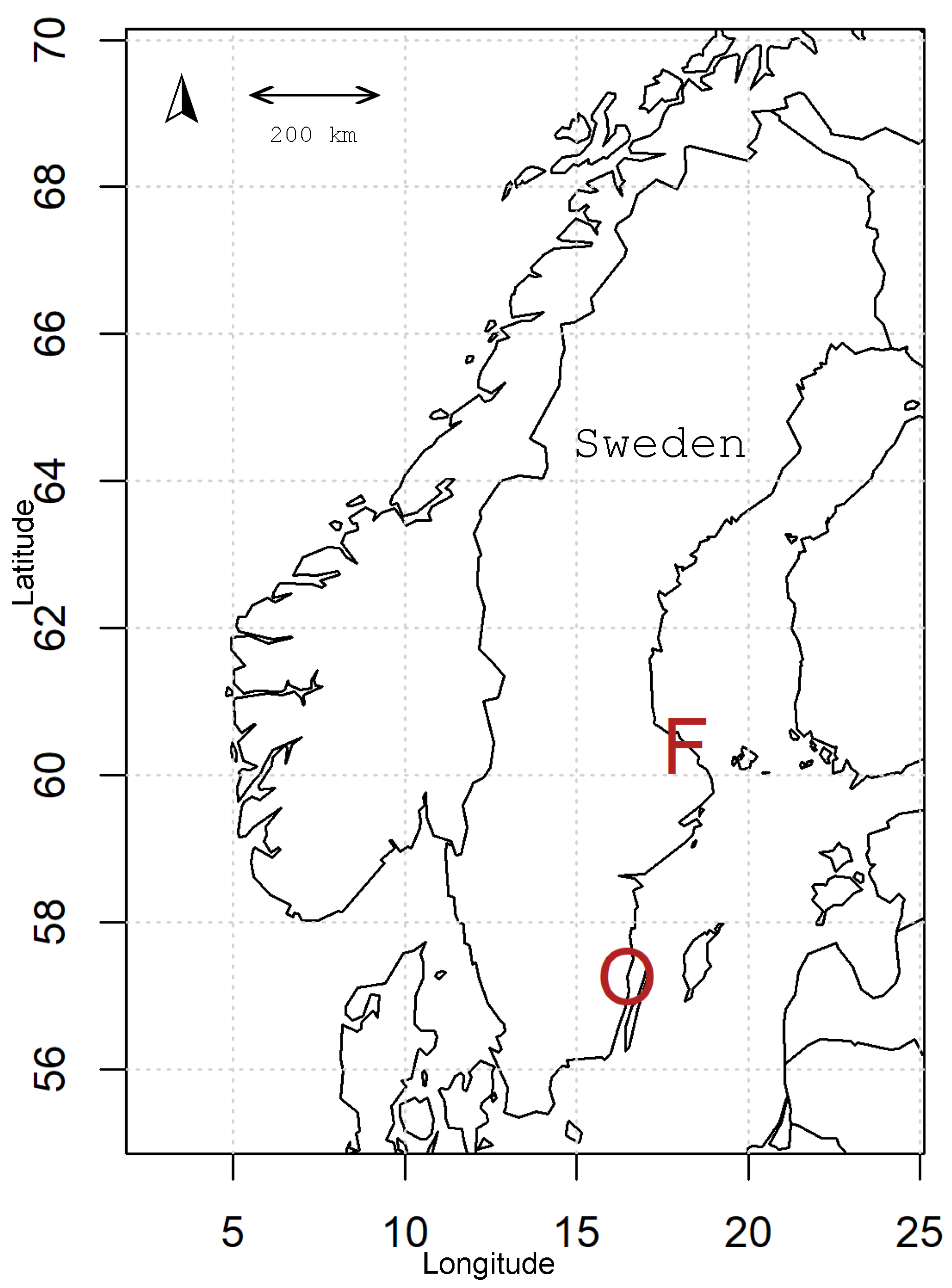
2.1.1. Sea Levels in the Baltic Sea

Sea levels in the Baltic Sea have been registered since the 18th century, with the series for Stockholm commencing already in 1774 [10]. Regarding changes in extreme sea levels along European coasts in general, Weisse et al. found that extreme sea levels show variability related to seasonal and nodal tidal cycles [11]. Moreover, long-term trends are mostly associated with corresponding mean sea level changes. Waves and storm surge climate do not show substantial long-term trends.

In a work oriented towards the Baltic Sea region, Weisse et al. state that over approximately the past 50 years, the Baltic absolute mean sea level has risen at a rate slightly larger than the global average [12]. However, in the northern parts of the Baltic Sea, due to vertical land movements, relative mean sea level has decreased. The phenomenon of land uplift has been known for some time. As early as in the 18th century, it was observed that the Earth’s surface was rising in the Nordic area. For instance, the famous Swedish geologist and polar researcher A.E. Nordenskiöld presented results of calculations [13]. Postglacial land uplift means the return of the earth crust to its state of equilibrium after having been heavily loaded by the kilometre-thick ice during the last Ice Age. The last ice disappeared from Scandinavia about 10,000 years ago.

A recent review on extreme events in the Baltic Sea region, not limited to sea level, is given in [14]. In the Baltic Sea, extreme sea levels could be caused by wind, air pressure (inverse barometric effect), and seiches. The amplitude of the internal tides is a few centimetres in most places, due to the Danish straits preventing the entrance of tidal waves into the Baltic Sea. Moreover, in the studies of observed extreme sea levels, no significant trends in extremes exceeding mean sea level rise have been found, except for the Gulf of Bothnia.

2.1.2. Measurements of Sea Level

Data in this study are hourly measurements of sea level (in cm) from recordings provided by the Swedish Meteorological and Hydrological Institute (SMHI). The sea levels are presented in relation to the zero level in the National Height System called RH2000. For the sake of simplicity, the RH2000 values were kept in the statistical analyses—the main objective is to compare statistical estimation techniques. However, the observations can be corrected for relative sea-level change (i.e., isostasy and eustasy). In the document [15] from SMHI, formulae are provided for such corrections. See [16], Section 2.3, for an example.

Two stations were considered, Forsmark and Oskarshamn, both located near to Swedish nuclear power plants.

Table 1. Stations considered in the study.

Station	Latitude/Longitude	Period
Forsmark	(60.41, 18.21)	1976–2022
Oskarshamn	(57.28, 16.48)	1961–2022

gives a summary including, e.g., the lengths of records. Further, the locations are shown on the map of Scandinavia in Figure 1. Data quality was overall decent, in the sense of few major portions missing. Concerning extremes, the winter season (from November to February) yields more extreme observations and need extra care in examination. The most serious example was Oskarshamn, with the period 27 January 1980 to 7 April 1980 missing in its entirety, but comparison with a neighbouring station (Ölands norra udde) showed that values were not extreme during that period. More precisely, the observations at Ölands norra udde during the gap period were all less than the 10 largest annual maxima during 1980 from Oskarshamn. Time series of annual maxima for the two stations are shown in Figure 2.

For these locations, we recall from Section 2.1.1 that the influence of tide could be neglected [14]. Furthermore, no significant trends in extremes exceeding mean sea level rise are of concern, since these data do not origin from the Gulf of Bothnia.

2.2. Statistical Methodology

2.2.1. Tests of Trend

In analysis of environmental data, a common non-parametric test of trend is the Mann–Kendall test (for a review, see, e.g., [17]). For a time series $\left\{x_t\right\}$, $t=1,2,\dots ,N$, the test statistic is given by

$$S=\sum _{k=1}^{N-1}\sum _{j=k+1}^N\mathrm{sgn}(x_j-x_k),$$

where

$$\mathrm{sgn}\left(x\right)=\left\{\begin{array}{cc}\hfill 1,& \mathrm{if} x>0,\hfill \\ \hfill 0,& \mathrm{if} x=0,\hfill \\ \hfill -1,& \mathrm{if} x<0.\hfill \end{array}\right.$$

For large N, the statistic S is approximately normally distributed. The sign of the test statistic indicates the tendency of trend; a negative sign is related to a negative slope, and vice versa. The implementation in the R package ‘trend’ was used [18].

Occasionally, when the Mann–Kendall test results show a significant trend, it is of interest to follow up with an analysis of possible changepoints. The non-parametric approach of Pettitt is commonly applied to detect a single changepoint in, e.g., hydrological series [19]. This tests the null hypothesis that the variables follow distributions that have the same location parameter (no change), against the alternative that a changepoint exists.

2.2.2. Extreme-Value Analysis and the GEV Distribution

Statistical extreme-value analysis can be said to concern the tails of distributions. The common approach is to fit a generalised extreme-value (GEV) distribution to a sample of independent annual maxima (“block maxima”). This then serves as the limiting distribution of independent maxima. The distribution function for the GEV distribution is given as

$$\mathsf{P}(X\le x)=exp\left\{-{\left[1+\xi \left(\frac{x-\mu }{\sigma }\right)\right]}^{-1/\xi }\right\},$$

(1)

defined on $\{x:1+\xi (x-\mu )/\sigma >0\}$, and where $\mu ,\sigma >0$ and $\xi$ are the location, scale and shape parameters, respectively.

The GEV distribution unifies three limiting distribution and the shape parameter $\xi$ is related to the nature of the tail. If $\xi <0$, the upper tail is bounded (reversed Weibull distribution); if $\xi =0$, the tail decays exponentially (Gumbel distribution); if $\xi >0$, the tail decays as a power function (Fréchet distribution). In the case $\xi <0$, the upper limit is given by $\mu -\sigma /\xi$.

When fitting a conventional GEV distribution to data, estimation is often performed using the ML method. When $-1<\xi \le -0.5$, the ML estimate exists, but does not have the standard asymptotic properties. Often in practice, $\xi >-0.5$ (cf. [1]), which is also the case in this study. For the numerical work in this paper. an implementation in R was used [20], as provided in the package ‘eva’ [21].

2.2.3. Return Levels

The T-year return level, corresponding to a return period T, is often defined as the high quantile for which the probability that the annual maximum exceeds this quantile is $1/T$. In the stationary case, the return level can be interpreted in two ways: that the expected waiting time until the next exceedance is T years, or that the expected number of events in T years is 1. For details and arguments, see [3].

For a GEV distribution, the return level follows from closed-form expressions as quantiles in the distribution:

$$y_T=\left\{\begin{array}{cc}\mu -\frac{\sigma }{\xi }[1-{(-ln(1-1/T))}^{-\xi }],\hfill & \xi \ne 0,\hfill \\ \mu -\sigma ln[1-ln(1-1/T\left)\right],\hfill & \xi =0.\hfill \end{array}\right.$$

(2)

Estimates of return levels are obtained by in Equation (2) by simply plugging in the ML estimates of the parameters $\mu$, $\sigma$ and $\xi$. The uncertainty of the return level is of interest to assess in risk analysis, and statistical procedures are, e.g., the delta method or profile likelihood. Usually, the profile-likelihood approach is preferred, as the delta method results in symmetric intervals [1]. The likelihood function is then reparameterised, and maximisation is carried out numerically with respect to two parameters, $\sigma$ and $\xi$.

2.2.4. The ACER Method

The ACER method was introduced in [6], with further examples presented in [7]. In this section, the method is briefly introduced. Mathematical details are given in Appendix A.

Denote the variable of interest (in this paper, sea level) with $\eta$. At the heart of the method is the so-called ACER function ${ϵ}_k\left(\eta \right)$, which can be interpreted as the rate at which the threshold $\eta$ is crossed, given the $k-1$ previous non-exceedances. It is defined by

$${ϵ}_k\left(\eta \right)=q_k\left(\eta \right)exp(-a_k{(\eta -b_k)}^{c_k})$$

(3)

where $a_k>0$, $b_k>0$, $c_k>0$, and the function $q_k\left(\eta \right)$ is slowly varying compared to the exponential function $exp(-a_k{(\eta -b_k)}^{c_k})$. In particular, the values $c_k=q_k\left(\eta \right)=1$ correspond to the asymptotic Gumbel distribution.

In practice, the choice of k needs to be addressed. The conditional upcrossings are assumed to be independent for high enough values of k. The case $k=1$ corresponds to the case of independent observations. Typically, through visualisations, a proper value of k is obtained; the ACER function is computed and drawn for different values of k, and one notes the value of k for which convergence is attained. Estimation of the parameters $a_k$, $b_k$, $c_k$ and $q_k$ in Equation (3) is then performed. Return levels corresponding to return period T can be computed by

$$y_T=b_k+{\left[\frac{1}{a_k}\left(ln\left(q_{k}N\right)-ln(-ln(1-1/T))\right)\right]}^{1/c_k}$$

(4)

where N is the average number of peaks in the data during one year. In this work, the implementation in the R package ‘acer’ was employed.

Furthermore, a so-called tail marker, ${\eta }_0$, needs to be specified in the algorithms. This corresponds to the place where the function starts to behave like the form in Equation (3), with a constant $q_k\left(\eta \right)=q_k$. See Section 3.3 for further discussion and numerical example.

3. Results

3.1. Trend Analysis

In

Table 2. Results of Mann–Kendall test for trend. Null hypothesis: no trend present. Two-sided alternative hypothesis (data follow a monotonic trend).

Station:	Forsmark	Oskarshamn
p-value:	$7.6·{10}^{-3}$	$8.4·{10}^{-1}$

, the results of the tests in form of p-values are presented. Recall from elementary statistics that given a significance level (usually 0.05), the null hypothesis is rejected if the p-value resulting from the test is less than the significance level. Thus, from the table, the test results in a trend for Forsmark. The value of S is negative ($S=-292$), and hence a negative slope. This seems reasonable when studying the times series of annual maxima in Figure 2 and could possibly be explained by land uplift in that part of the Baltic.

Following up with Pettitt’s test for Forsmark, results in the p-value 0.052, which corresponds to year 2007. The possible suggestion of a shift here might be due to the somewhat higher observed maximum this year, compared to years before and after, cf. Figure 2.

In the sequel, we apply the ACER methodology. As pointed out in [6], this technique is applicable to non-stationary time series.

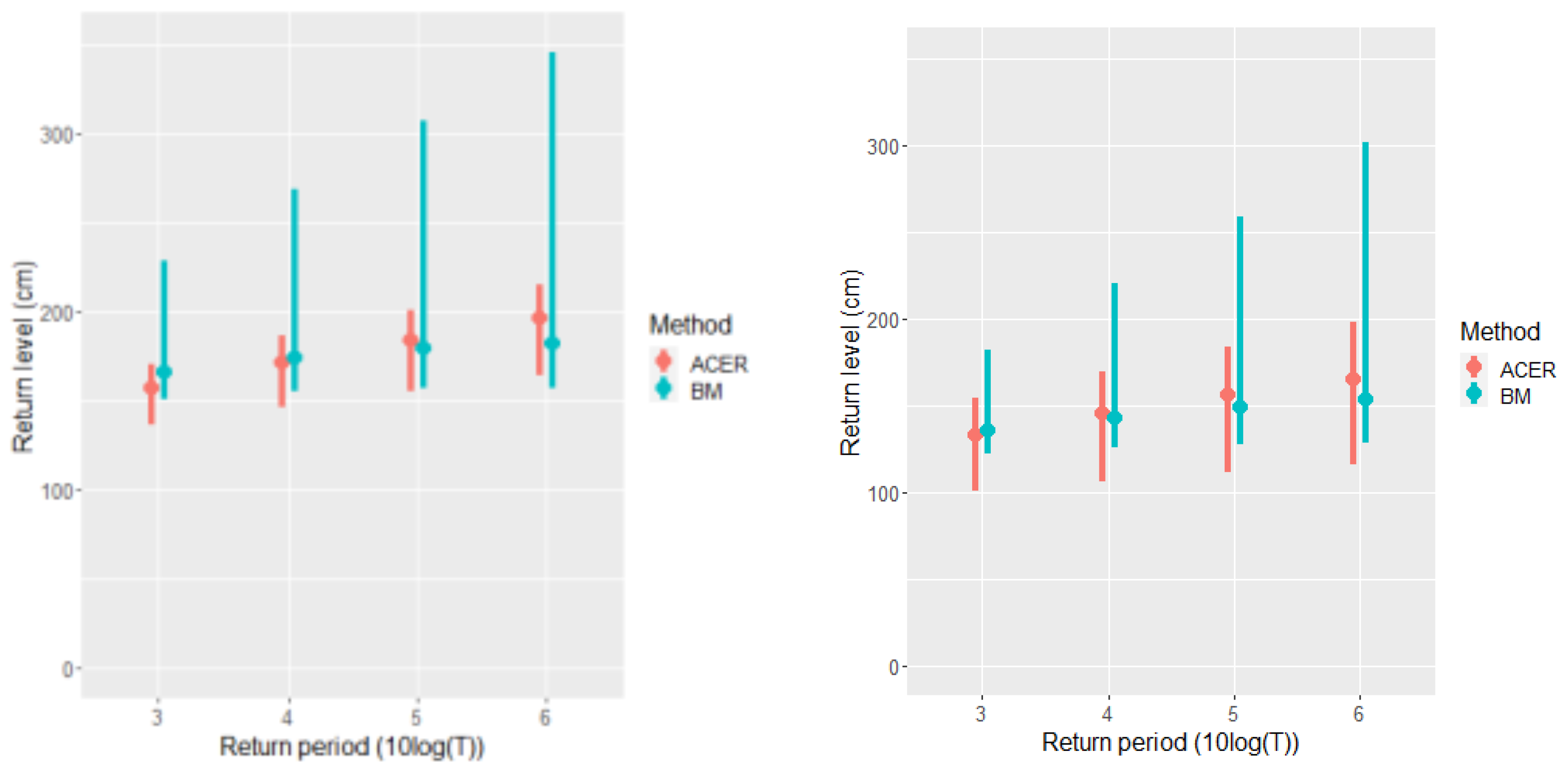
3.2. Estimation of Return Levels: Comparisons

A comparison of the conventional method of block maxima (BM) and the ACER methodology is the main aim of this paper. We present in Figure 3 the resulting estimates of return levels (for return periods in years ${10}^3$, ${10}^4$, ${10}^5$, ${10}^6$) along with related 95% confidence intervals. In the case of block maxima, confidence intervals were computed by profile likelihood. We now describe the findings; first the point estimates, then the uncertainties of estimates in form of confidence intervals.

Point estimates. ACER estimates tend to be higher than those resulting from BM, the longer the return period. The difference is, however, in all cases less than 2 dm. Recall from Section 2.2.2 that a negative shape parameter implies an upper bound for a GEV distributed random variable. The maximum-likelihood estimates are for Forsmark and Oskarshamn $-0.23$ and $-0.17$, respectively. Simple Wald tests result in rejection of the null hypothesis with $\xi =0$ for these stations.

Confidence intervals. It is clear from Figure 3 that the uncertainties are considerably reduced with the ACER methodology. For both methodologies under study, the intervals become wider with increasing return period, but more notably so for the conventional BM approach. One may note that the confidence intervals by ACER are skewed to the left. This phenomenon is found also in other applications of the method, e.g., in the report [9].

In the study [8] of extreme sea levels along the Norwegian coast, intervals with return period 200 years were compared and the same features as in the present paper were found; compared to a BM approach, minor differences in point estimates, but less wide confidence intervals for return levels.

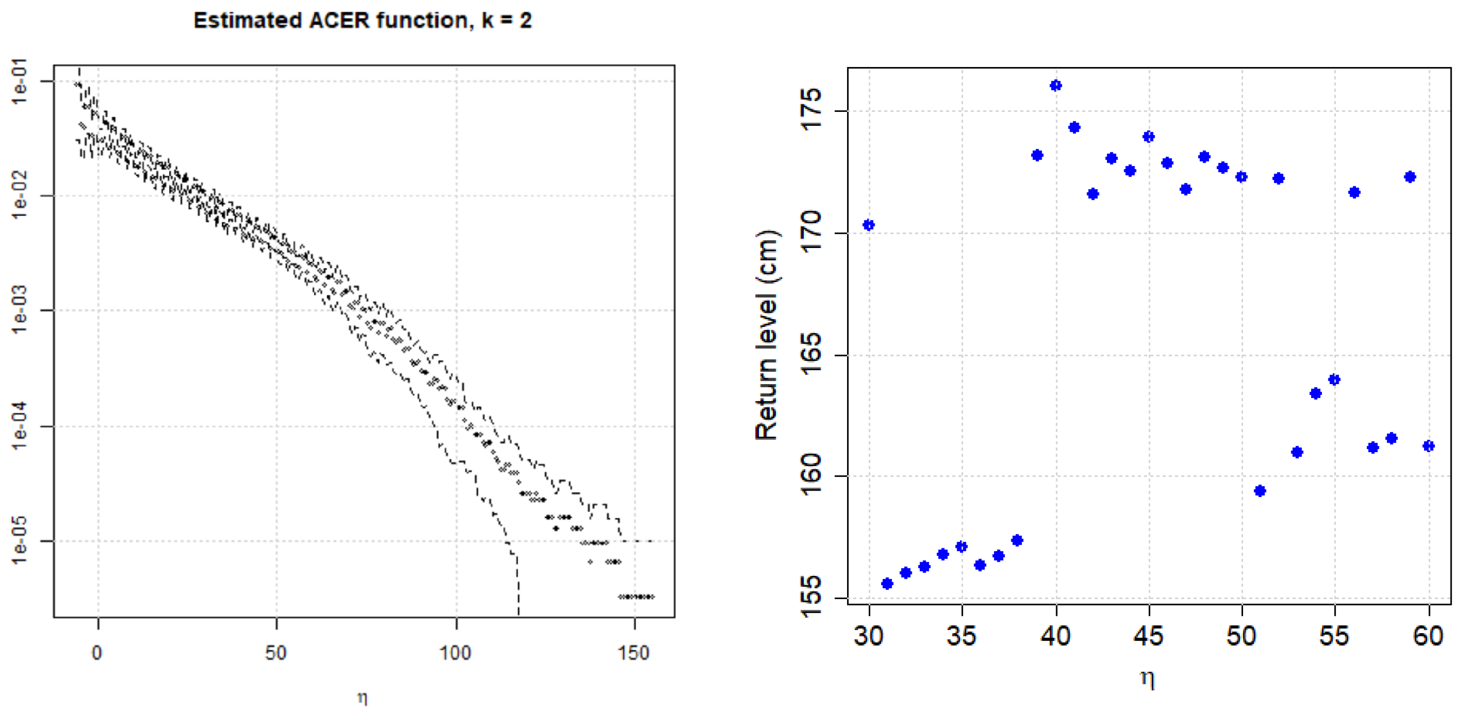
3.3. Notes on the ACER Methodology

Recall from Section 2.2.4 that $k=1$ corresponds to the case of independent observations. To apply the algorithms, a proper k value needs to be chosen for estimation of return levels (as well as value of the tail marker ${\eta }_0$). An introductory ACER plot resulted for all stations in the choice $k=2$; the same choice was made in [8] for data of similar character.

Turning to the selection of the tail marker ${\eta }_0$, a plot of the ACER function ${ϵ}_k\left(\eta \right)$ can assist. One should try to find where the ACER function seems to behave regularly. Choosing a higher value would increase the variance of the estimate (the number of observation points decreases). In Figure 4, outcomes for Forsmark station are shown as an example. Judging from the left panel, a value less than 50 seems to be the case. In addition one could, as pointed out in [8], check the stability of return-level estimates for a range of tail markers. This is shown for the situation with return period 1000 years in Figure 4, right panel. In this particular case, ${\eta }_0=38$ was chosen.

4. Summary and Discussion

Estimation of return levels for long return periods (longer than 1000 years, say) is a non-trivial task, since uncertainties typically become large. We have demonstrated that the confidence intervals are considerably shorter with the ACER approach, compared to the classical block-maxima method (Figure 3). More precisely, for Forsmark station, the ratio of interval lengths ranged from 2.3 to 3.7 (return periods ${10}^3$ up to ${10}^6$), while for Oskarshamn, the ratios ranged from 1.1 to 2.1 for the same choice of return periods investigated. The methodology has also proven useful for series coming from heavy tailed distributions [22].

Skjong et al. compared the ACER methodology to three other techniques (block-maxima with Gumbel or GEV; POT, revised joint probabilities method), and found for three locations along the Norwegian coast that the ACER in all cases resulted in the shortest confidence intervals [8]. Return periods up to 200 years were considered. Still, alternative procedures exist. Rydén and Freyland investigated the performance of the so-called r largest-maximum approach for the same Swedish locations as in the present paper [23]. Comparing with block-maximum (with GEV), that approach resulted in shorter confidence intervals. However, for return periods longer than 10,000 years, intervals became too wide for practical use.

The sign of the shape parameter could be crucial due to its relationship with a possible upper bound [24]. Similarly to the present paper, Skjong et al. found negative estimates of the shape parameter along the Norwegian coast, ranging from $-0.28$ to $-0.09$ [8]. The question on sign of shape parameter has been discussed for other quantities as well, e.g., maximum daily rainfall. For this quantity, Papalexiou and Koutsoyiannis investigated an impressive number of 15,137 records from all over the world, fitting GEV distributions [25]. They found that when the effect of the record length was corrected, the shape parameter $\xi$ varied in a narrow range; moreover, an influence of geographical location on the value of $\xi$. A variability in sign of $\xi$ was found, but in the majority of cases (about 80%), $\xi >0$.

From a climatology point of view, when discussing extreme sea levels along the Scandinavian coastlines, one might refer to recent research reported in [26]. Six sites along the Swedish coast were then investigated using a so-called flood-risk simulation framework. The general conclusion was for longer planning periods, the risk of flooding is dominated by high sea-level rise. This is in line with statements found in [11].

Finally, there are several other approaches for estimation of return levels of environmental extremes. For instance, in [27] is suggested a procedure that like the ACER method makes use of the complete time series. A Bayesian framework is another option, as stated in [5]: “Thus, where feasible, we propose a Bayesian estimation strategy for optimal return level inference”.

References

1. Dey, D.; Roy, D.; Yan, J. Univariate extreme value analysis. In Extreme Value Modeling and Risk Analysis. Methods and Applications; Dey, D.K., Yan, J., Eds.; CRC Press, Chapman & Hall: New York, NY, USA, 2016; pp. 1–22. [Google Scholar]
2. Belzile, L.R.; Dutang, C.; Northrop, P.J.; Opitz, T. A modeler’s guide to extreme value software. Extremes 2023, 26, 595–638. [Google Scholar] [CrossRef]
3. Cooley, D. Return periods and return levels under climate change. In Extremes in a Changing Climate; AghaKouchak, A., Easterling, D., Hsu, K., Schubert, S., Sorooshian, S., Eds.; Springer: Berlin/Heidelberg, Germany, 2013; pp. 97–114. [Google Scholar]
4. Volpi, E. On return period and probability of failure in hydrology. WIREs Water 2019, 6, e1340. [Google Scholar] [CrossRef]
5. Fawcett, L.; Walshaw, D. Sea-surge and wind speed extremes: Optimal estimation strategies for planners and engineers. Stoch. Environ. Res. Risk. Assess. 2016, 30, 463–480. [Google Scholar] [CrossRef]
6. Naess, A.; Gaidai, O. Estimation of extreme values from sampled time series. Struct. Saf. 2009, 31, 325–334. [Google Scholar] [CrossRef]
7. Naess, A.; Gaidai, O.; Karpa, O. Estimation of extreme values by the average conditional exceedance rate method. J. Probab. Stat. 2013, 2013, 797014. [Google Scholar] [CrossRef]
8. Skjong, M.; Naess, A.; Brandrud Naess, O.E. Statistics of extreme sea levels for locations along the Norwegian coast. J. Coast. Res. 2013, 29, 1029–1048. [Google Scholar] [CrossRef]
9. Simpson, M.J.R.; Nilsen, J.E.Ø.; Ravndal, O.R.; Breili, K.; Sande, H.; Kierulf, H.P.; Steffen, H.; Jansen, E.; Carson, M.; Vestøl, O. Sea Level Change for Norway. Past and Present Observations and Projections to 2100. NCCS Report No. 1/2015. Available online: https://www.miljodirektoratet.no/globalassets/publikasjoner/M405/M405.pdf (accessed on 22 January 2024).
10. Ekman, M. Climate changes detected through the world’s longest sea level series. Glob. Planet. Chang. 1999, 21, 215–224. [Google Scholar] [CrossRef]
11. Weisse, R.; Bellafiore, D.; Menéndez, M.; Méndez, F.; Nicholls, R.J.; Umgiesser, G.; Willems, P. Changing extreme sea levels along European coasts. Coast. Eng. 2014, 87, 4–14. [Google Scholar] [CrossRef]
12. Weisse, R.; Dailidienė, I.; Hünicke, B.; Kahma, K.; Madsen, K.; Omstedt, A.; Parnell, K.; Schöne, T.; Soomere, T.; Zhang, W.; et al. Sea level dynamics and coastal erosion in the Baltic Sea region. Earth Syst. Dyn. 2021, 12, 871–898. [Google Scholar] [CrossRef]
13. Nordenskiöld, A.E. Beräkning af fasta landets höjning vid Stockholm. Öfversigt Kongl. Vetenskaps Akad. Förhandlingar 1858, 15, 269–272. [Google Scholar]
14. Rutgersson, A.; Kjellström, E.; Haapala, J.; Stendel, M.; Danilovich, I.; Drews, M.; Jylhä, K.; Kujala, P.; Larsén, X.G.; Halsnæs, K.; et al. Natural hazards and extreme events in the Baltic Sea region. Earth Syst. Dyn. 2022, 13, 251–301. [Google Scholar] [CrossRef]
15. SMHI: Ekvationer för Medelvattenståndet i Rikets Höjdsystem 2000 (RH2000), 2023. Available online: https://www.smhi.se/polopoly_fs/1.195046!/mwreg_MWekvationer_2023.pdf (accessed on 6 February 2024).
16. Posada, M. Statistical Analysis of Oceanographic Data: A Comparison between Stationary and Mobile Sea Leve Gauges. Master’s Thesis, Lund University, Lund, Sweden, 2014. [Google Scholar]
17. Chandler, R.; Scott, M. Statistical Methods for Trend Detection and Analysis in the Environmental Sciences; Wiley: Hoboken, NJ, USA, 2011. [Google Scholar]
18. Pohlert, T. Trend. Non-Parametric Trend Tests and Change-Point Detection. R-Package. Available online: https://cran.r-project.org/web/packages/trend/ (accessed on 14 February 2024).
19. Pettitt, A.N. A non-parametric approach to the change point problem. J. R. Stat. Soc. Ser. C Appl. Stat. 1979, 28, 126–135. [Google Scholar] [CrossRef]
20. R Core Team. R: A Language and Environment for Statistical Computing; R Foundation for Statistical Computing: Vienna, Austria. Available online: https://www.R-project.org/ (accessed on 14 February 2024).
21. Bader, B.; Yan, J. EVA. Extreme Value Analysis wih Goodness-of-Fit Testing. R Package. Available online: https://cran.r-project.org/web/packages/eva/ (accessed on 14 February 2024).
22. Dahlen, K.E. Comparison of ACER and POT Methods for Estimation of Extreme Values. Master’s Thesis, NTNU, Trondheim, Norway, 2010. [Google Scholar]
23. Rydén, J.; Freyland, S. Estimation of return levels of sea level along the Swedish coast by the method of r largest annual maxima. In Proceedings of the 33rd International Ocean and Polar Engineering Conference, ISOPE-2023, Ottawa, ON, Canada, 19–23 June 2023; pp. 2762–2766. [Google Scholar]
24. Rydén, J. A tale of two stations: A note on rejecting the Gumbel distribution. Acta Geophys. 2023, 71, 385–390. [Google Scholar] [CrossRef]
25. Papalexiou, S.M.; Koutsoyiannis, D. Battle of extreme value distributions: A global survey on extreme daily rainfall. Water Resour. Res. 2013, 49, 187–201. [Google Scholar] [CrossRef]
26. Hieronymus, M.; Kalén, O. Should Swedish sea level planners worry more about mean sea level rise or sea level extremes? Ambio 2022, 51, 2235–2332. [Google Scholar] [CrossRef] [PubMed]
27. Volpi, E.; Fiori, A.; Grimaldi, S.; Lombardo, F.; Koutsoyiannis, D. Save hydrological observations! Return period estimation without data decimation. J. Hydrol. 2019, 571, 782–792. [Google Scholar] [CrossRef]
Figure 1. Map over Scandinavia with the locations of measurement stations indicated. F: Forsmark. O: Oskarshamn.
Geohazards 05 00008 g001
Figure 2. Time series, annual maxima of sea level at the two locations under study.
Geohazards 05 00008 g002
Figure 3. Estimated return levels with related confidence intervals (profile-likelihood method). Left panel: Forsmark. Right panel: Oskarshamn.
Geohazards 05 00008 g003
Figure 4. Illustrations for Forsmark. Left panel: Plot of the estimated ACER function ϵ ^ k ( η ) (for k = 2 ) for assessing a proper value of the tail marker η 0 . Right panel: Stability of return-level estimates. Choice by the author: η 0 = 38 .
Geohazards 05 00008 g004