Induced Seismicity Hazard Assessment for a Potential CO₂ Storage Site in the Southern San Joaquin Basin, CA

Abstract

California’s Central Valley offers vast opportunities for CO₂ storage in deep saline aquifers. We conducted an induced seismicity hazard assessment for a potential injection site in the southern San Joaquin Basin for 18 years of injection at 0.68 MtCO₂/yr and 100 years of monitoring. We mapped stress, faults, and seismicity in a 30 km radius around the site to build a geomechanical model and resolve the stresses on major faults. From a 3D hydromechanical simulation of the CO₂ plume, we calculated the change in pressure over time on these faults and determined the conditions for safe injection. Lacking any subsurface imaging, we also conducted a probabilistic fault slip analysis using numerous random distributions of faults and a range of geomechanical parameters. Our results show that the change in probability of fault slip can be minimized by controlling the size, migration, and magnitude of the pressure plume. We also constructed a seismic catalog for the last 20 years around the site and characterized the natural patterns of seismicity. We use these results to establish criteria for evaluating potential-induced events during the storage period and to develop a traffic light response system. This study represents a first-order procedure to evaluate the seismic hazards presented by CO₂ storage and incorporate uncertainties in hydrological and geomechanical parameters.

1. Introduction

The San Joaquin Basin has significant potential storage capacity for CO₂ in deep saline aquifers (16.6–52 Gt) [1]. Although the parts of the basin suited for storage are not tectonically active, there are major faults that present seismic hazards. Increasing pore pressure in storage reservoirs through CO₂ injection pushes faults closer to failure by decreasing fault-effective normal stress. Injection-induced seismicity has previously occurred in California during fluid injection associated with enhanced geothermal recovery [2] and wastewater disposal [3]. Although there have been no large, damaging earthquakes induced by CO₂ storage, there have been many observations of microseismicity related to CO₂ injection [4,5,6]. In CO₂ storage applications, induced seismicity represents a hazard in terms of human nuisance and safety, damage to surface and subsurface structures, and storage integrity [7]. While the area of the CO₂ plume remains relatively small, the pressure perturbation and deformation field extend much further [8]. These perturbation fields evolve over time. So, it is critical to assess the potential for fault slip through both injection and storage periods.

In this study, we take a three-part approach to evaluating seismic hazards at a candidate site in the Southern San Joaquin Basin of California. First, we build a geomechanical model and evaluate the stress state of mapped faults near the injection site. We then examine the probability of induced fault slip due to CO₂ injection using random populations of faults and a distribution of geomechanical parameters. From these analyses, we delineate the pressure conditions that minimize the potential to induce slip on faults, given the spatial extent and magnitude of the predicted pressure plume. Finally, we characterize the natural patterns of seismicity at the site and establish criteria for differentiating induced events during the injection storage periods and for responding to events at different thresholds using a traffic light system.

2. Method

The first step of our analysis was to map stress, seismicity, and faults in the area surrounding the injection site. Based on estimates of the CO₂ pressure plume size from a three-dimensional hydromechanical model implemented in Computer Modeling Group (CMG) software [9], we chose to study the area within a ~20 km radius of the injector. We obtained principal stress directions and relative stress magnitudes from recently published U.S. stress maps that include borehole measurements and earthquake focal mechanism inversions [10]. For the seismic catalog, we used the USGS earthquake catalog from 1920 to 2008 and a recently published Southern California catalog from 2008 to 2018 [11], and the Southern California Earthquake Data Center (SCEDC) catalog from 2018 to present. The new Southern California catalog uses template matching to detect more events and relocate previously detected events. Fault locations and orientations were obtained from the USGS Quaternary Faults database [12]. No seismic imaging was available for the area, so we simply assume that each of the mapped faults extends from the surface and intersects the entire thickness of the storage formation at depth. We used the stress map data to calculate the resolved shear and normal stresses on the mapped faults at depth and determine what pressure conditions are safe during the injection period. Because we do not have a complete picture of the fault architecture or material properties at depth, we also conducted a probabilistic fault slip analysis to understand the conditions for fault slip given a range of geomechanical and fault properties. Finally, we analyzed the last 20 years of earthquake data around the site to understand the characteristics of naturally occurring seismicity. We performed a declustering analysis of the updated seismic catalogs and used seismic density as a metric to track changes in seismic characteristics that may distinguish natural and induced seismicity during the monitoring phase.

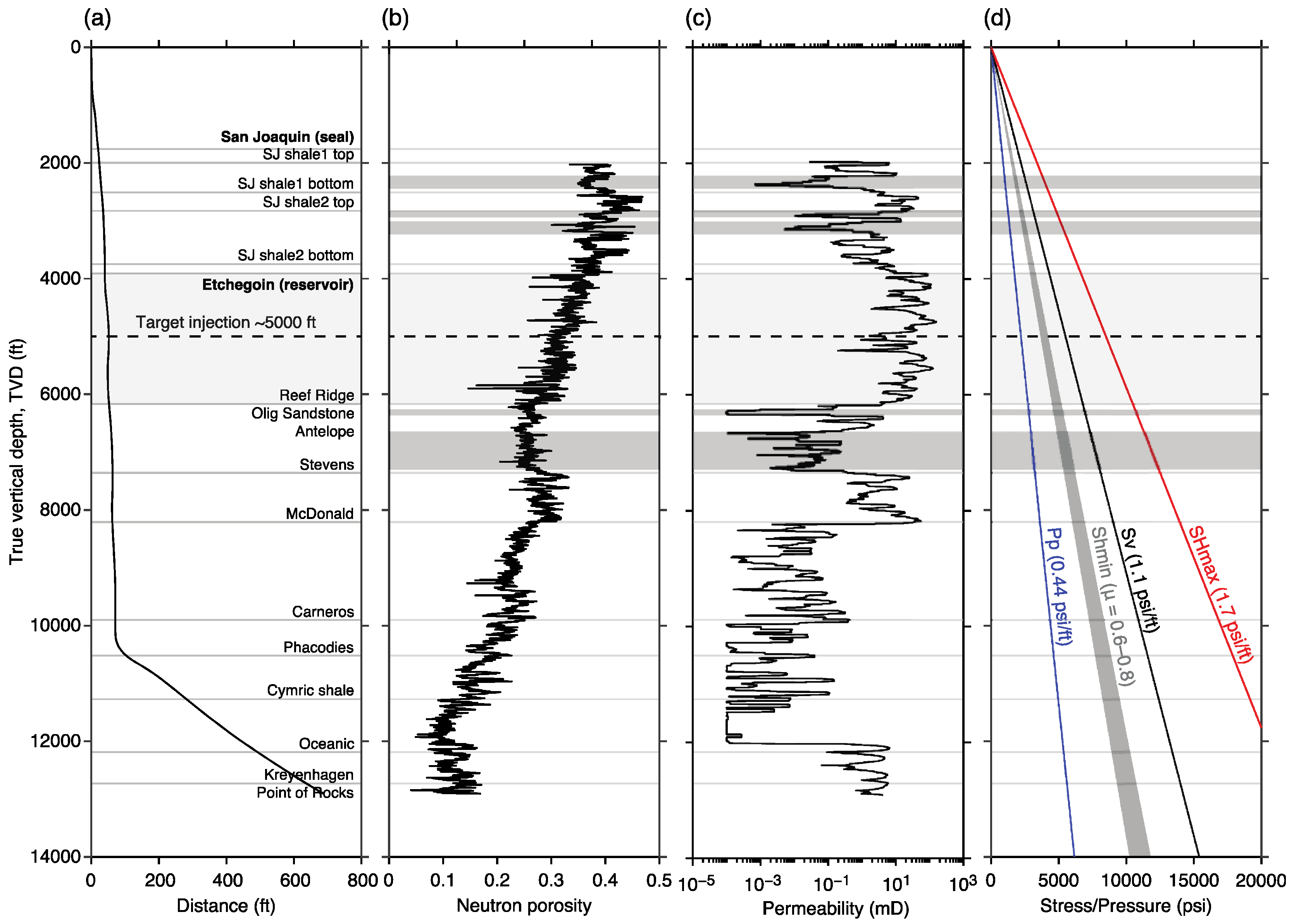
3. Site Characteristics

The proposed injection site is northwest of Bakersfield, CA, in the Southern San Joaquin Basin (Figure 1). This area of the basin is predominantly composed of Cenozoic marine sediments that show a depositional sequence transitioning from a deep marine to a shallow brackish environment [13]. The target formation for storage is the Etchegoin, a Pliocene-age marine formation comprised of interbedded siltstones, sandstones, and silty sands. In the region of the proposed site, the Etchegoin is ~1000–2000 ft thick and dips ~9° to the southeast [14]. The porosity from neutron logs is measured between 25 and 33% and the permeability is estimated between 1 and 10 mD (Figure 2). Above the Etchegoin are multiple low-permeability shales and claystones of the San Joaquin formation, which serve as the overlying seals. Below the Etchegoin is the low-permeability Antelope shale (0.1–1 µD). The target injection depth in the Etchegoin is 5000 ft (1524 m).

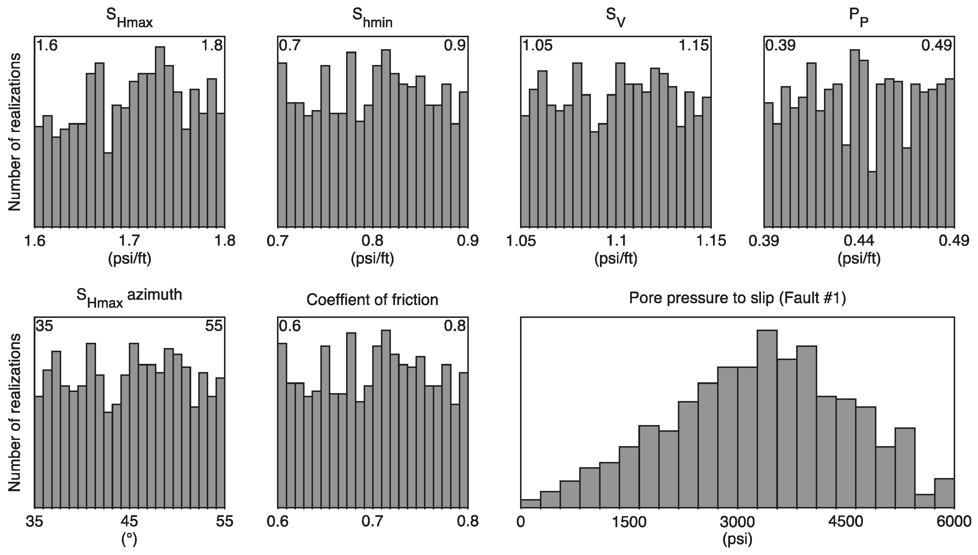
3.1. Stress

The candidate area is in a strike-slip stress state, signifying that the maximum horizontal stress (S_Hmax) is the greatest principal stress component. The magnitude of A_Φ, which describes the ratio of the principal stresses, is ~1.5–1.7 [15]. The maximum horizontal stress is oriented approximately normal to the San Andreas Fault to the southwest. S_Hmax orientations around the injection site are relatively consistent, ~50–60° N-NE. We estimated the gradient of the vertical stress (S_v) at 1.1 psi/ft based on reasonable values for sedimentary rock density. We then used earthquake focal mechanism inversion to obtain the relative magnitudes of the three principal stresses. Based on our estimate for S_v, the S_Hmax gradient is ~1.7 psi/ft. To estimate S_hmin, we use frictional faulting theory, assuming a range of values for the fault coefficient of friction of 0.6–0.8 and obtain a value of ~0.8–0.9 psi/ft. Well data and the lack of production from the Etchegoin suggest that the pore pressure is likely hydrostatic (0.44 psi/ft).

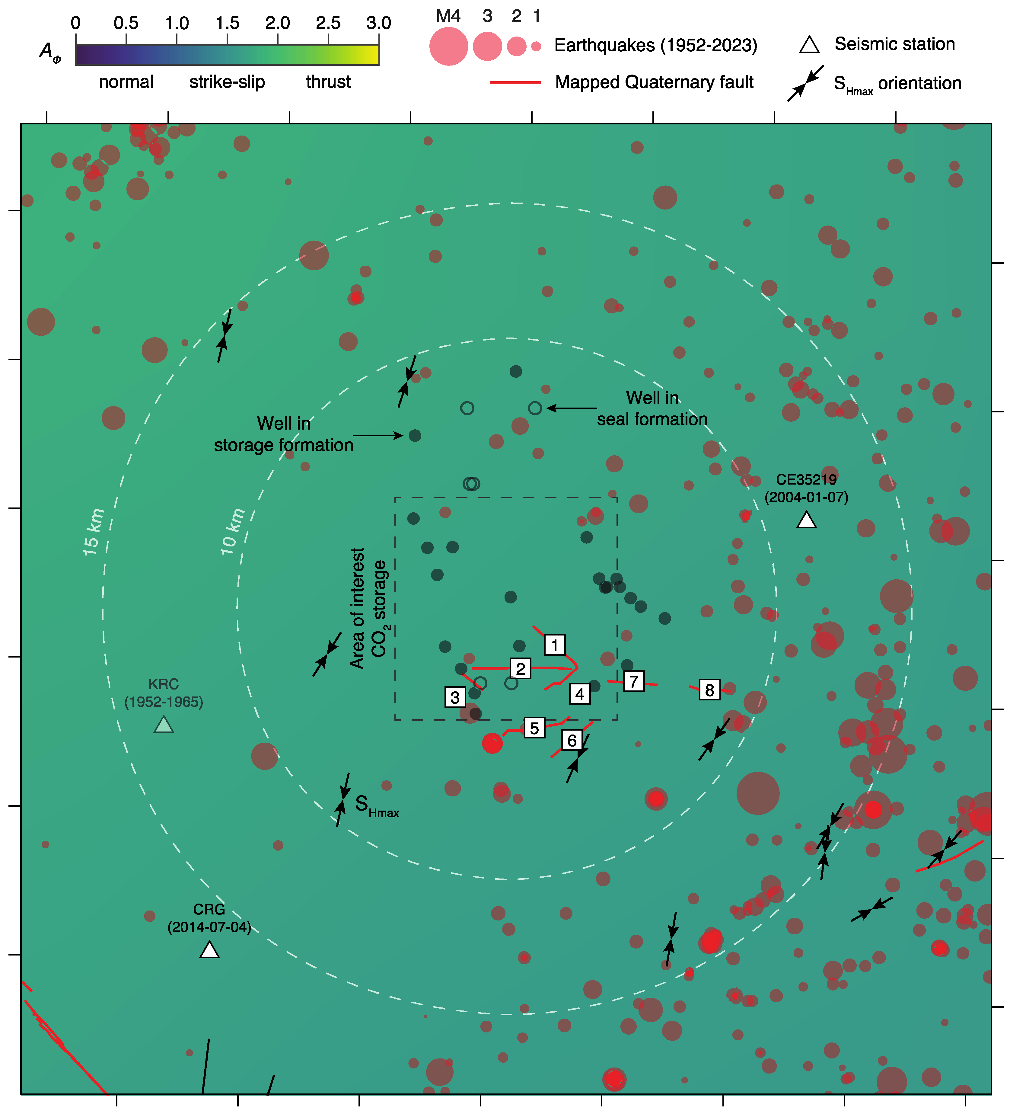
3.2. Faults

Within 10 km of the candidate site, there are 8 mapped fault structures (Figure 1). To evaluate the conditions for slip on these faults, we used the estimated principal stress magnitudes to calculate the resolved stresses on each fault (Figure 3). We assumed that each of these faults penetrates the formation at the injection depth and that the friction coefficient is 0.6–0.8. Lower frictional resistance makes faults more susceptible to induced slip. We found that several faults (2, 7, and 8) are well-oriented for slip, meaning that only a small pore pressure change is needed to induce slip, as shown in Figure 3. These faults are steeply dipping, E-W-striking features that are oblique to the S_Hmax. Faults 4 and 6 are oriented nearly parallel to S_Hmax and do not have enough shear stress to slip, while fault 5 is oriented nearly normal to S_Hmax and has too much normal stress to slip. Based on our analysis, faults 1 and 3 could not slip in this stress field because the pore pressure required to trigger slip is greater than the minimum principal stress (S_hmin). We plotted the pressure to induce slip on each fault as a function of distance from the injector to highlight the range of pressure plume profiles that are safe. Our analysis indicates that pressure changes should be kept below 400 psi within 1–2 km of the injector in order to limit the potential for induced slip on well-oriented fault 2.

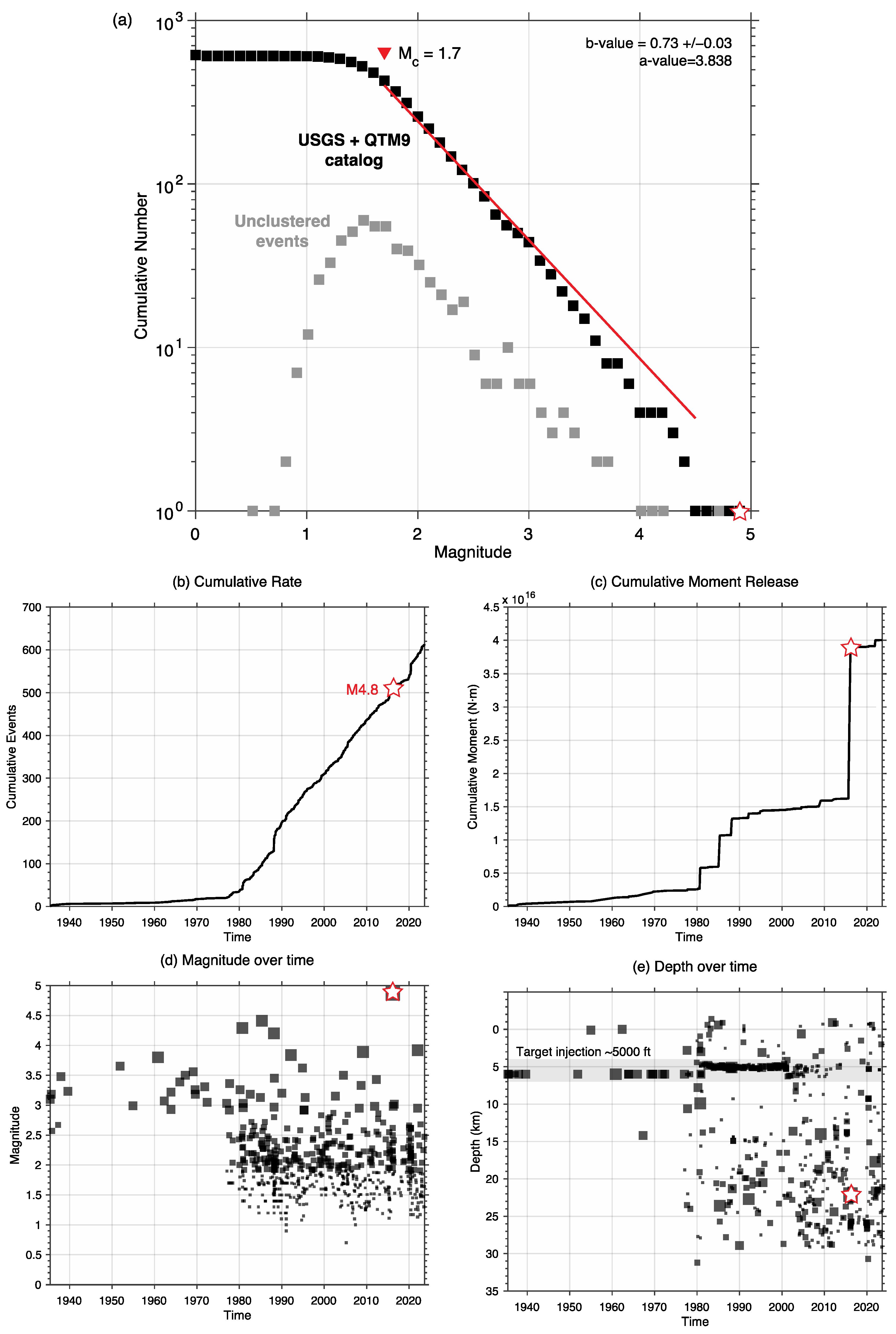
3.3. Seismicity

The area around the proposed injector is seismically quiescent relative to the surroundings (Figure 1). There are only 3 broadband seismometers in the area, all more than 10 km away from the injector. The combined earthquake catalog for the area around the injector has approximately one thousand events since 1980, with a b-value of 0.73 and a magnitude of catalog completion of ~1.7 as shown in Figure 4a. Earthquake catalogs were compiled and analyzed using the software package ZMAP [16]. The largest event is M4.9, which occurred over 20 km to the NE of the proposed injector. The majority of large events occurred at depths greater than 5 km, significantly below the proposed injection zone at 5000 ft (1.524 km). There are no major earthquakes or earthquake sequences on any of the eight mapped Quaternary faults (Figure 1).

We performed a declustering analysis of the catalog in ZMAP utilizing the Gardner and Knopoff method [17]. The declustered data represent mainshock events that are not associated with space or time. Due to limited seismic coverage in the area, there are less than 100 declustered events, with a similar magnitude of catalog completion to the full catalog. These declustered events will be used to calculate the tectonic background seismicity in the area of interest.

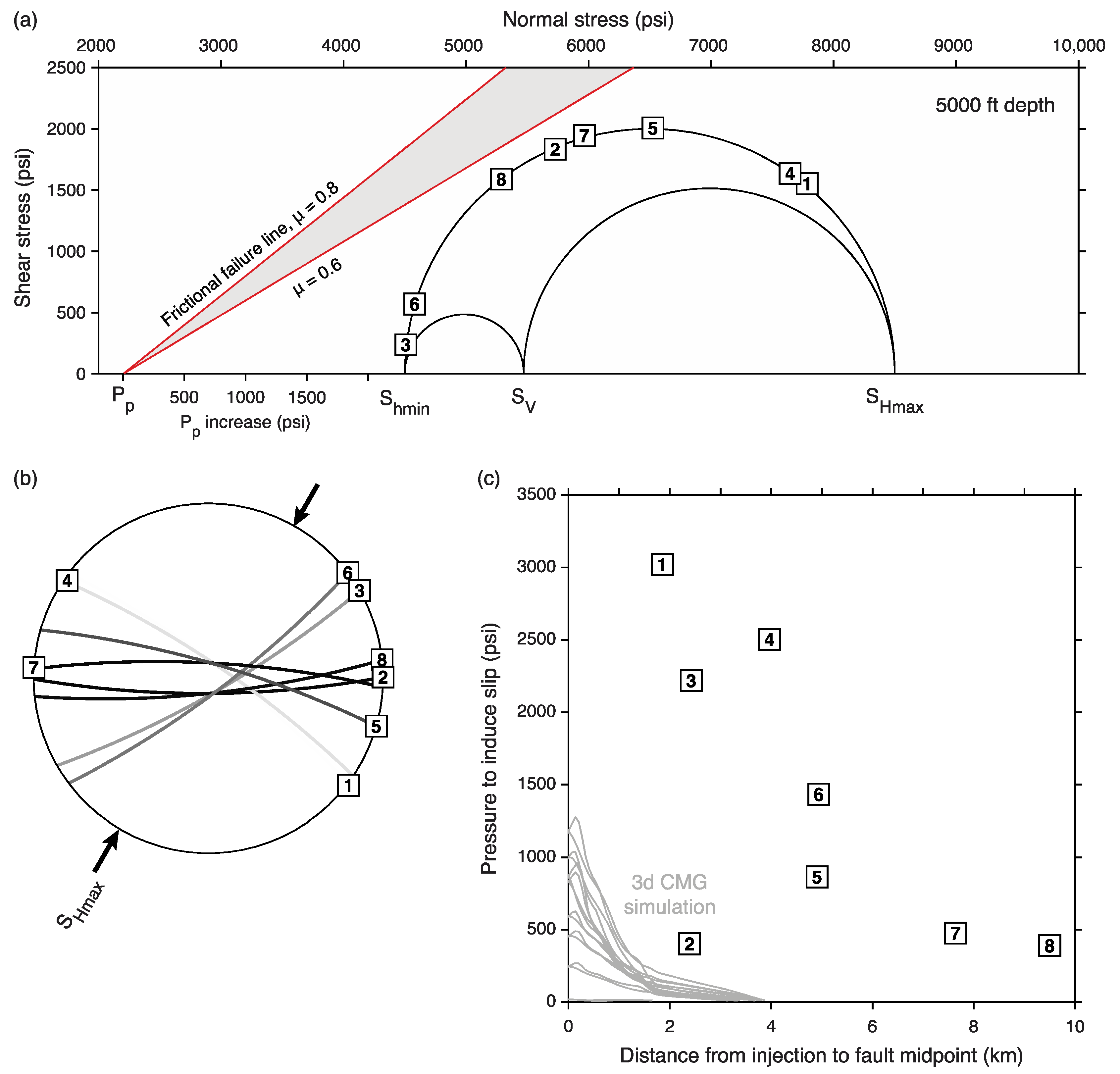
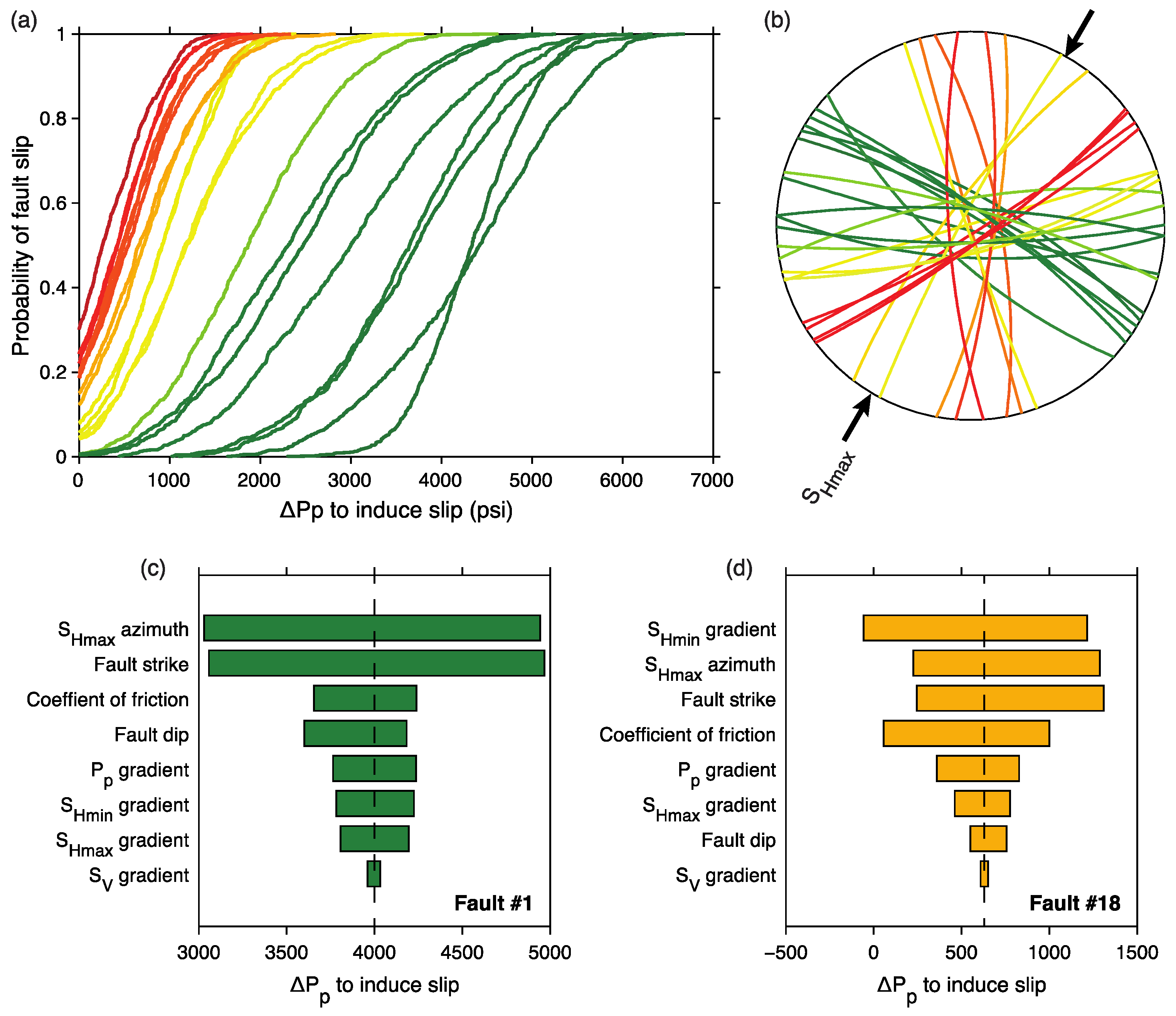
4. Fault Slip Potential

Because our knowledge of subsurface faults and their properties is limited, it is useful to examine the probability of fault slip for a range of geomechanical parameters and fault scenarios. We constructed a probabilistic model for fault slip using the Fault Slip Potential (FSP) software from the Stanford Center for Induced and Triggered Seismicity [18]. There are no seismic profiles, image logs, or earthquake sequences to reveal subsurface structures, so we chose to use numerous random distributions of faults with characteristics similar to those mapped at the surface. Figure 5 shows the range of geomechanical parameters used in the analysis. We generated populations of 20 near vertical faults (dip = 75–85°) and allowed the strike of each to vary by ±10°. We used ranges of ±0.1 psi/ft for S_v, S_hmin, and pore pressure. We allowed the S_Hmax azimuth to vary by ±10°. Both the coefficient of friction and the A_Φ parameter vary by ±0.1.

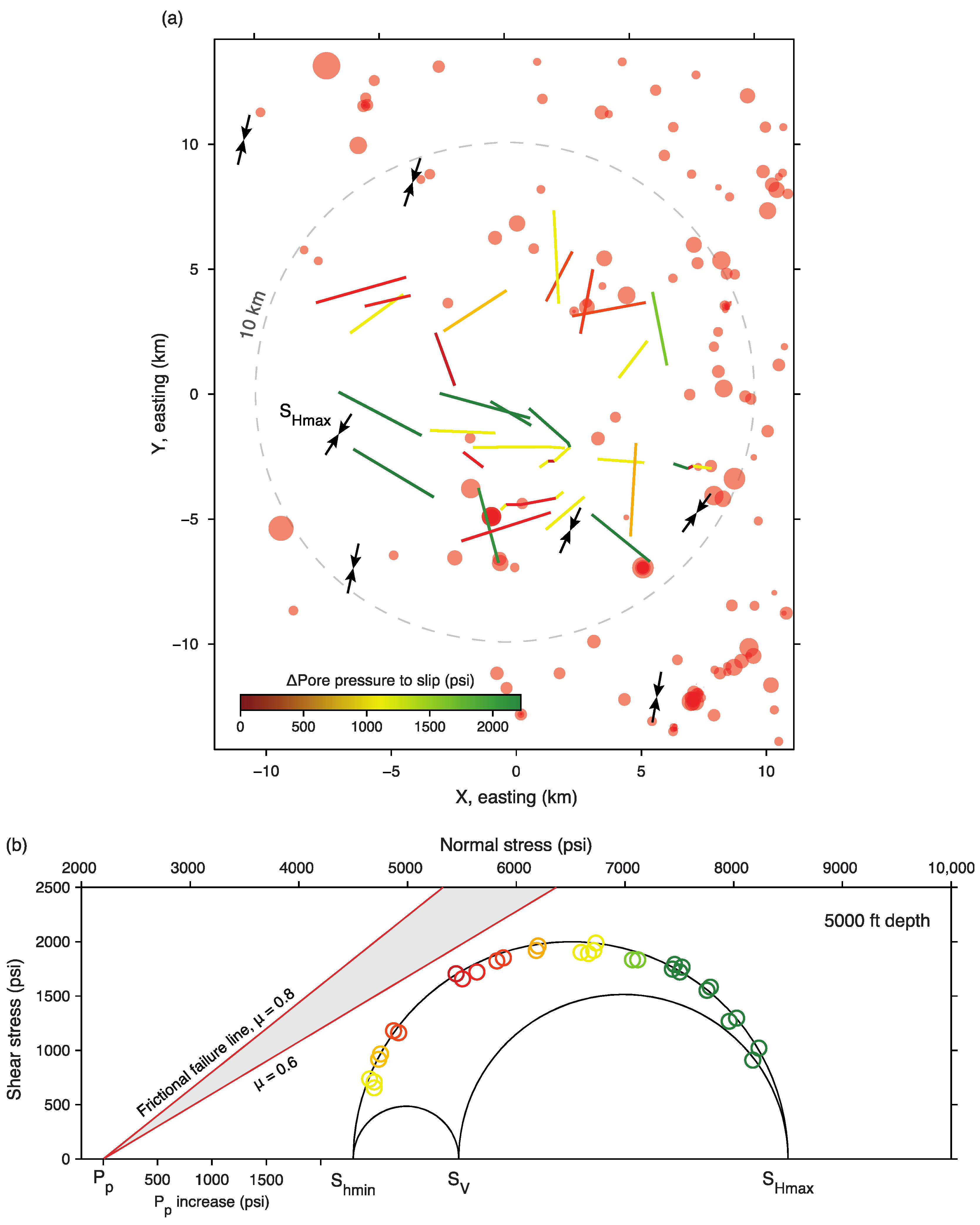
4.1. Initial Stress State

From each random distribution of faults, we calculate the pore pressure change to induce slip in the given stress field. We used populations of 20 faults with fault lengths 1–4 km in a 10 × 10 km area around the injector. Figure 6 shows a map view of the faults and a Mohr-Coulomb diagram with one population of faults colored by the change in pore pressure required to induce slip. Similar to the analysis of quaternary faults, faults perpendicular to S_Hmax have too much normal stress to slip in the given stress field. Faults oblique to S_Hmax are well oriented for slip and will slip with pore pressure changes of ~600–1000 psi.

FSP uses a Monte Carlo scheme to propagate the uncertainty in geomechanical parameters throughout the model. Each realization is a point on a probability distribution function that represents the likelihood of inducing fault slip given a specific change in pore pressure (Figure 7a). We ran 2000 realizations for each fault scenario. FSP also generates tornado diagrams for each fault that show the sensitivity of the change in pore pressure with respect to the varying geomechanical parameters (Figure 7c). The probability of fault slip in the initial stress state ranges from 0 to 0.3. For poorly-oriented fault 1, the pore pressure to slip is most sensitive to the S_Hmax azimuth, while for well-oriented fault 18, the highest sensitivity is for the S_hmin gradient. In both cases, pore pressure to slip is not very sensitive to the S_Hmax gradient and to well-constrained parameters, e.g., fault dip and vertical stress gradient.

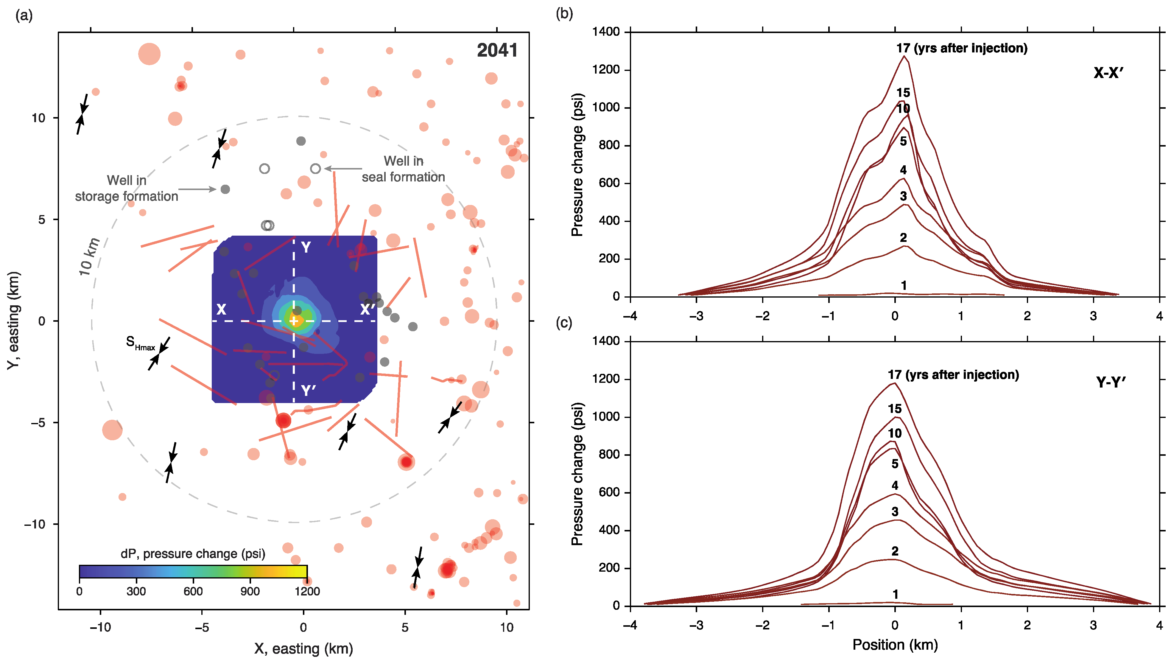
4.2. Post-Injection

We use the results of the 3D hydromechanical simulation of CO₂ injection (Figure 8) to quantify the likelihood of fault slip given the simulated pressure plume. The model prescribes 18 years of injection at ~0.68 MtCO₂/yr and 100 years of monitoring. We used data on pressure change over time from a two-dimensional layer (Figure 8a) approximately at the target injection depth (5000 ft) to calculate the change in fault slip potential.

We input time series data of the pressure plume (e.g., Figure 8b,c) into FSP to quantify the change in the fault slip potential value, or the probability of inducing fault slip, over time (Figure 9). We calculate the change in pressure at each fault midpoint over time in Figure 9b and combine the results with the probability distribution function given in Figure 7a to determine the fault slip potential over time in Figure 9c. In this injection scenario, the rate of pressurization at the faults increases in a logarithmic fashion during injection and drops immediately after the end of injection. The maximum pressure changes on faults range from ~200 to 400 psi. Fault slip potential values on the faults closest to failure increase from ~0.3 to 0.5 over the injection period.

5. Seismic Analysis

Using the expanded southern California earthquake catalog, we examined the recent seismic history of the area and explored different metrics to quantify the natural patterns of seismicity. Due to the limited number of stations and sparse event data in the region of the simulated pressure plume, we are not able to conduct statistically significant Gutenberg–Richter mapping to establish a baseline for the natural frequency-magnitude distribution, e.g., [3,14,15]. This could be a useful metric to evaluate changes in seismicity patterns due to injection, but it requires a dense, near-well monitoring network established before the start of injection.

5.1. Seismic Density

Another potentially useful metric for understanding induced seismicity is the spatiotemporal seismicity rate, or seismic density [19]. We gridded the seismic density as a function of distance from the injection zone using 2 km grids radially and 1 month time windows for the area within 40 km of the injector (Figure 10). The background seismicity rate for this region is ~0.1–0.2 events/month/km². Following large events, seismicity rates can increase up to 0.5 events/month/km². On the right side of Figure 10, which represents the period after the start of injection, we plot the spatial extent of the CO₂ saturation and pressure plumes calculated from the hydromechanical model. The extent of the saturation plume corresponds to regions with CO₂ saturations > 5%, and the extent of the pressure plume corresponds to regions with pressure increases > 10 psi. Based on these models, we do not expect the region of the pressure plume to interact with any of the areas that have had large events with intense aftershock sequences. Therefore, we can use seismicity density as a real-time monitoring metric to highlight event sequences in the region of influence that may be induced by CO₂ injection.

5.2. Distinguishing Natural and Induced Events

To evaluate whether events during the injection period are natural or induced, we developed a three-part criterion detailed in

Table 1. Criteria for assessing potential induced seismic events, including thresholds for area of interest (AOI), seismic characteristics, and ground shaking.

Criteria	Description	Action
Area of Interest
Thermal plume	Region of thermal stresses > 5% of initial reservoir model	If event with threshold characteristics or shaking occurs in thermal plume, refer to traffic light protocol (Table 2).
Pressure plume	Region where change in pressure is >10 psi than initial reservoir model	If event with threshold characteristics or shaking occurs in pressure plume, refer to traffic light protocol.
Strain plume	Region where strains are >0.1% than initial reservoir model	If event with threshold characteristics or shaking occurs in strain plume, refer to traffic light protocol.
Mapped fault	Large event or swarm on mapped fault in seal, reservoir, or underburden	If event with threshold characteristics or shaking occurs on mapped fault, refer to traffic light protocol.
Seismic Characteristics
Event magnitude	Event magnitude obtained from USGS or local network	If event > M3 in AOI refer to red light protocol. If <M3, assess seismic characteristics and ground shaking.
Seismic density	Spatial density of events in time	If density > 0.2 mo−1 km−1 in area of interest, assess other seismic characteristics and shaking criteria and refer to traffic light protocol if necessary.
Gutenberg-Richter	G-R statistics for earthquake swarms	Additional aseismic data is needed to determine thresholds for changes in G-R statistics.
Ground Shaking
Peak ground acceleration (PGA)	PGA for nearby population centers, sensitive infrastructure	If PGA > 0.1 g, assess area of interest and seismic characteristics and refer to traffic light protocol if necessary.
Perceived shaking	Felt reports to USGS or operator	If perceived shaking > Strong (PGA 0.9–1.8) reported, assess area of interest and seismic characteristics, and refer to traffic light protocol if necessary.
Reported damage	Damage reported to USGS or operator	If damage reported, assess all criteria, and refer to traffic light protocol.

. There are 3 subcategories: area of interest, seismic characteristics, and ground shaking. If an event triggers the threshold of any one of the subcategories, we will examine the other subcategories further. Area of interest (AOI) signifies that the seismic event occurred in the region that is mechanically influenced by CO₂ injection, as predicted by the three-dimensional hydromechanical model, or on a mapped fault of interest. Also, events in the seal units or in the underlying basement that could result in leakage [6] or rapid pressure migration [3] merit additional investigation. If the plume intersects any high-permeability structures that were not previously identified through geophysical imaging, it is possible for large events to be induced outside the AOI. Hydrologically conductive fractures are often critically stressed, meaning only a small pore pressure change is needed to induce slip. In the case of saltwater disposal in Oklahoma, although the seismicity rate of significant earthquakes M > 3 correlated with the loading rate, some of the largest events M > 5 occurred after the peak of injection outside the area of the modeled pressure plume [20].

Seismic characteristics refer to single events or populations of events and include magnitude, spatial seismicity rate, and magnitude-frequency statistics (Gutenberg–Richter). During the monitoring period, we plan to compare future events to the seismic characteristics of past sequences to identify any anomalous behavior that may have been induced by injection. A caveat here is the need for high-resolution monitoring around an injector in advance of the injection period. Recently, a seismicity rate model combined with a geomechanical simulation has been used to successfully hindcast the rates and magnitudes of minor induced events M< 2 at the Decatur, IL CO₂ storage site [21], which underscores the potential to anticipate the character of induced seismicity with sufficient monitoring. In addition to such physics-based approaches for forecasting induced seismicity, earthquake cycle models may be useful for quantifying background seismicity and identifying anomalous behavior. The concept of “natural time”, or representing the number of small earthquakes as the timescale between large earthquakes [22], is particularly relevant to induced seismicity in tectonically active areas with long duration data, where the earthquake cycle defines the probability distribution of large events. This methodology was used to successfully identify and “nowcast” induced seismicity due to gas production in the Groningen field in the Netherlands [23] and could readily be applied to CO₂ storage sites with sufficient seismic monitoring. Since the natural time between large events scales with magnitude, long-duration recording is needed to predict potentially damaging events.

Ground shaking refers to the recorded acceleration at seismic stations as well as the perceived shaking by people. Any events that cause felt reports or reported damage should be examined further.

6. Traffic Light Protocol

If an event is in the area of interest and exceeds thresholds for seismic characteristics or ground shaking, the event or event sequence will be studied in greater detail to establish causality with injection. Events determined as induced will trigger a response according to a traffic light protocol, e.g., Table 2. These schema have been successfully used to manage the risk of induced seismicity due to wastewater injection and hydraulic fracturing [24] and have been proposed for CO₂ storage [25]. We adapted a traffic light protocol from the Archer Daniels Midland EPA Class VI well application for the Decatur, IL, storage site [26]. We updated the threshold conditions to reflect the characteristics of the updated earthquake catalog for the prospective site. We also include additional metrics such as seismicity density and the difference between the pressure recorded at the monitoring well and the predicted pressure from simulation. Each set of threshold conditions results in a corresponding action sequence. A critical step resulting from exceeding the orange threshold is reviewing the space-time correlation between injection parameters (rate, pressure, and volume) and potentially induced events or event sequences. In the case of confirmed induced events with problematic outcomes (i.e., risk of leakage, perceptible, and/or damaging ground shaking), the only sure course of action is to reduce injection rates and continue monitoring both pressures and seismicity. If seismicity continues or intensifies after injection stops, e.g., [27], it may be feasible to temporarily produce CO₂ and brine to further reduce pressure changes on faults in the near-well region. Seismicity occurring outside or above/below the modeled region of influence could indicate rapid fluid migration, and operations should be halted until the relevant structures are resolved through geophysical imaging.

Table 2. Summary of traffic light states, threshold conditions, and response actions. Adapted from the ADM EPA Class VI application for the Decatur, IL, site [26].

State	Threshold Conditions	Action
	- Seismic events < M1.5 (2) in AOI (1) - Spatial seismicity rate < 0.2 mo−1 km−2 - Pressure change (dP) less than or equal to model	1. Continued operations at current levels
	- Seismic events M1.5–2.0 (2) in AOI (1) - Spatial seismicity rate 0.2–0.4 mo−1 km−2 - Monitoring well dP 1% greater than model	1. Continued operations at current levels 2. Within 24 h of the incident, notify the Underground Injection Control (UIC) Program Director of the operating status of the well.
	- Event > M2.0 (2) in AOI (1) and/or felt report (3) - Spatial seismicity rate > 0.5 mo−1 km−2 - Seismic event > M1.5 on mapped fault - Seismic event > M1.5 above/below storage unit - Monitoring well dP 5–10% greater than model	1. Injection rate reduction 2. Vent CO2 from surface facilities 3. Within 24 h of the incident, notify the UIC Program Director of the operating status of the well. 4. Limit access to wellhead 5. Coordinate evacuation plans, if necessary 6. Monitor well diagnostics (pressure, temperature, strain etc.) 7. Check for impacts on USDW [28] 8. If USDW contamination detected, shutdown operations. 9. Review seismic and operational data for space-time correlation. 10. Report findings to UIC Program Director and amend operating conditions if necessary.
	- Seismic event > M3.0 (2) in AOI (1) and/or felt report (3) and/or damage report (4) - Spatial seismicity rate > 1 mo−1 km−2 - Seismic event > M2.0 on mapped fault - Seismic event > M2.0 above/below storage unit - Monitoring well dP > 10% greater than model	1. Shutdown procedure 2. Vent CO2 from surface facilities and shut in well 3. Within 24 h of the incident, notify the UIC Program Director of the operating status of the well. 4. Limit access to wellhead 5. Coordinate evacuation plans, if necessary 6. Monitor well diagnostics (pressure, temperature, strain, etc.) 7. Check for impacts on USDW [28] 8. If USDW contamination detected, shutdown operations. 9. Review seismic and operational data for space-time correlation. 10. Report findings to UIC Program Director and amend operating conditions if necessary.

(1) AOI as defined by 3D reservoir simulation results; see Table 1 for details. (2) Determined by the site monitoring network and/or USGS seismic monitoring stations and/or reported by the USGS National Earthquake Information Center using the national seismic network. (3) Confirmed by local reports of felt ground motion or reported on the USGS “Did You Feel It?” reporting system. (4) The onset of damage is defined as cosmetic damage to structures.

Table 2. Summary of traffic light states, threshold conditions, and response actions. Adapted from the ADM EPA Class VI application for the Decatur, IL, site [26].

State	Threshold Conditions	Action
	- Seismic events < M1.5 (2) in AOI (1) - Spatial seismicity rate < 0.2 mo−1 km−2 - Pressure change (dP) less than or equal to model	1. Continued operations at current levels
	- Seismic events M1.5–2.0 (2) in AOI (1) - Spatial seismicity rate 0.2–0.4 mo−1 km−2 - Monitoring well dP 1% greater than model	1. Continued operations at current levels 2. Within 24 h of the incident, notify the Underground Injection Control (UIC) Program Director of the operating status of the well.
	- Event > M2.0 (2) in AOI (1) and/or felt report (3) - Spatial seismicity rate > 0.5 mo−1 km−2 - Seismic event > M1.5 on mapped fault - Seismic event > M1.5 above/below storage unit - Monitoring well dP 5–10% greater than model	1. Injection rate reduction 2. Vent CO2 from surface facilities 3. Within 24 h of the incident, notify the UIC Program Director of the operating status of the well. 4. Limit access to wellhead 5. Coordinate evacuation plans, if necessary 6. Monitor well diagnostics (pressure, temperature, strain etc.) 7. Check for impacts on USDW [28] 8. If USDW contamination detected, shutdown operations. 9. Review seismic and operational data for space-time correlation. 10. Report findings to UIC Program Director and amend operating conditions if necessary.
	- Seismic event > M3.0 (2) in AOI (1) and/or felt report (3) and/or damage report (4) - Spatial seismicity rate > 1 mo−1 km−2 - Seismic event > M2.0 on mapped fault - Seismic event > M2.0 above/below storage unit - Monitoring well dP > 10% greater than model	1. Shutdown procedure 2. Vent CO2 from surface facilities and shut in well 3. Within 24 h of the incident, notify the UIC Program Director of the operating status of the well. 4. Limit access to wellhead 5. Coordinate evacuation plans, if necessary 6. Monitor well diagnostics (pressure, temperature, strain, etc.) 7. Check for impacts on USDW [28] 8. If USDW contamination detected, shutdown operations. 9. Review seismic and operational data for space-time correlation. 10. Report findings to UIC Program Director and amend operating conditions if necessary.

(1) AOI as defined by 3D reservoir simulation results; see Table 1 for details. (2) Determined by the site monitoring network and/or USGS seismic monitoring stations and/or reported by the USGS National Earthquake Information Center using the national seismic network. (3) Confirmed by local reports of felt ground motion or reported on the USGS “Did You Feel It?” reporting system. (4) The onset of damage is defined as cosmetic damage to structures.

7. Conclusions

Our study highlights the need for detailed, site-specific assessments of induced seismicity hazards for CO₂ injection projects in California. In the AOI of the prospective site, mapped faults are not associated with any located earthquakes, suggesting that these faults are not active in the current tectonic regime. However, increasing pore pressure through CO₂ injection drives faults closer to failure and may induce slip if the magnitude and footprint of the pressure plume are not controlled. Our geomechanical analysis suggests that the potential to reactivate mapped faults in the area is low if pressures are kept below 500 psi within 1–2 km of the injector. The probabilistic fault slip analysis indicates fault slip may change by up to 20% under the proposed injection conditions. The greatest hazard is presented by well-oriented faults within 2 km of the injector, where pressure changes are greatest and occur relatively rapidly. Sensitivity analysis indicates that stress magnitudes and orientations are the greatest sources of variability in fault slip probability, which underscores the need for borehole stress measurements at the injection site and monitoring well locations.

Although the change in seismic hazards under the proposed injection conditions may be within risk tolerances, more data is needed to resolve faults and seismicity in the estimated AOI. Based on our analysis, we recommend the following strategies to further characterize and mitigate the risk of induced seismicity at the prospective site:

• Fortify the earthquake catalog by deploying more surface seismic stations around the injector and borehole seismic stations nearby a monitoring well;
• Conduct image logs and stress measurements in both the injector and monitoring well to characterize depth variations in stress and locate zones with active faults;
• Acquire seismic imaging to identify hidden faults in the subsurface;
• Design the permanent monitoring array around the predicted plume footprint;
• Take corrective action if the pressure plume extent and the magnitude of the pressure increase deviate from simulation results, and adhere to the corrective actions proposed in the traffic light system.

References

- Kim, T.W.; Yaw, S.; Kovscek, A.R. Evaluation of Geological Carbon Storage Opportunities in California and a Deep Look in the Vicinity of Kern County. In Proceedings of the SPE Western Regional Meeting, Bakersfield, CA, USA, 26–28 April 2022; SPE: Bakersfield, CA, USA, 2022; p. D011S005R001. [Google Scholar]
- Eberhart-Phillips, D.; Oppenheimer, D.H. Induced Seismicity in The Geysers Geothermal Area, California. J. Geophys. Res. 1984, 89, 1191–1207. [Google Scholar] [CrossRef]
- Goebel, T.H.W.; Hosseini, S.M.; Cappa, F.; Hauksson, E.; Ampuero, J.P.; Aminzadeh, F.; Saleeby, J.B. Wastewater Disposal and Earthquake Swarm Activity at the Southern End of the Central Valley, California. Geophys. Res. Lett. 2016, 43, 1092–1099. [Google Scholar] [CrossRef]
- Stork, A.L.; Verdon, J.P.; Kendall, J.-M. The Microseismic Response at the In Salah Carbon Capture and Storage (CCS) Site. Int. J. Greenh. Gas Control 2015, 32, 159–171. [Google Scholar] [CrossRef]
- White, J.A.; Foxall, W. Assessing Induced Seismicity Risk at CO2 Storage Projects: Recent Progress and Remaining Challenges. Int. J. Greenh. Gas Control 2016, 49, 413–424. [Google Scholar] [CrossRef]
- Glubokovskikh, S.; Saygin, E.; Shapiro, S.; Gurevich, B.; Isaenkov, R.; Lumley, D.; Nakata, R.; Drew, J.; Pevzner, R. A Small CO2 Leakage May Induce Seismicity on a Sub-Seismic Fault in a Good-Porosity Clastic Saline Aquifer. Geophys. Res. Lett. 2022, 49, e2022GL098062. [Google Scholar] [CrossRef]
- Zoback, M.; Smit, D. Meeting the Challenges of Large-Scale Carbon Storage and Hydrogen Production. Proc. Natl. Acad. Sci. USA 2023, 120, e2202397120. [Google Scholar] [CrossRef] [PubMed]
- Rutqvist, J. The Geomechanics of CO2 Storage in Deep Sedimentary Formations. Geotech. Geol. Eng. 2012, 30, 525–551. [Google Scholar] [CrossRef]
- Li, Y. Pilot Scale Geological Carbon Storage and Injection Well Design Optimization. Ph.D. Thesis, Stanford University, Stanford, CA, USA, 2023. [Google Scholar]
- Lundstern, J.-E.; Zoback, M.D. Multiscale Variations of the Crustal Stress Field throughout North America. Nat. Commun. 2020, 11, 1951. [Google Scholar] [CrossRef]
- Ross, Z.E.; Trugman, D.T.; Hauksson, E.; Shearer, P.M. Searching for Hidden Earthquakes in Southern California. Science 2019, 364, 767–771. [Google Scholar] [CrossRef]
- Quaternary Fault and Fold Database for the United States. Available online: https://www.usgs.gov/natural-hazards/earthquake-hazards/faults (accessed on 1 June 2023).
- Downey, C.; Clinkenbeard, J. An Overview of Geologic Carbon Sequestration Potential in California; California Energy Commission: Sacramento, CA, USA, 2005.
- Myer, L.; Downey, C.; Clinkenbeard, J.; Thomas, S.; Stevens, S.; Benson, S.; Zheng, H.; Herzog, H.; Biediger, B. Preliminary Geologic Characterization of West Coast States for Geologic Sequestration; California Energy Commission: Sacramento, CA, USA, 2005.
- Simpson, R.W. Quantifying Anderson’s Fault Types. J. Geophys. Res. 1997, 102, 17909–17919. [Google Scholar] [CrossRef]
- Wiemer, S. A Software Package to Analyze Seismicity: ZMAP. Seismol. Res. Lett. 2001, 72, 373–382. [Google Scholar] [CrossRef]
- Gardner, J.K.; Knopoff, L. Is the Sequence of Earthquakes in Southern California, with Aftershocks Removed, Poissonian? Bull. Seismol. Soc. Am. 1974, 64, 1363–1367. [Google Scholar] [CrossRef]
- Walsh, F.R.; Zoback, M.D.; Pais, D.; Weingarten, M.; Tyrell, T. FSP 1.0: A Program for Probabilistic Estimation of Fault Slip Potential Resulting from Fluid Injection. Available online: https://scits.stanford.edu/fault-slip-potential-fsp (accessed on 1 June 2023).
- Goebel, T.H.W.; Hauksson, E.; Aminzadeh, F.; Ampuero, J.-P. An Objective Method for the Assessment of Fluid Injection-induced Seismicity and Application to Tectonically Active Regions in Central California. J. Geophys. Res. Solid Earth 2015, 120, 7013–7032. [Google Scholar] [CrossRef]
- Langenbruch, C.; Weingarten, M.; Zoback, M.D. Physics-Based Forecasting of Man-Made Earthquake Hazards in Oklahoma and Kansas. Nat. Commun. 2018, 9, 3946. [Google Scholar] [CrossRef]
- Luu, K.; Schoenball, M.; Oldenburg, C.M.; Rutqvist, J. Coupled Hydromechanical Modeling of Induced Seismicity from CO2 Injection in the Illinois Basin. JGR Solid Earth 2022, 127, e2021JB023496. [Google Scholar] [CrossRef]
- Rundle, J.B.; Turcotte, D.L.; Donnellan, A.; Grant Ludwig, L.; Luginbuhl, M.; Gong, G. Nowcasting Earthquakes. Earth Space Sci. 2016, 3, 480–486. [Google Scholar] [CrossRef]
- Luginbuhl, M.; Rundle, J.B.; Turcotte, D.L. Natural Time and Nowcasting Induced Seismicity at the Groningen Gas Field in the Netherlands. Geophys. J. Int. 2018, 215, 753–759. [Google Scholar] [CrossRef]
- Walters, R.J.; Zoback, M.D.; Baker, J.W.; Beroza, G.C. Characterizing and Responding to Seismic Risk Associated with Earthquakes Potentially Triggered by Fluid Disposal and Hydraulic Fracturing. Seismol. Res. Lett. 2015, 86, 1110–1118. [Google Scholar] [CrossRef]
- Templeton, D.C.; Schoenball, M.; Layland-Bachmann, C.E.; Foxall, W.; Guglielmi, Y.; Kroll, K.A.; Burghardt, J.A.; Dilmore, R.; White, J.A. A Project Lifetime Approach to the Management of Induced Seismicity Risk at Geologic Carbon Storage Sites. Seismol. Res. Lett. 2023, 94, 113–122. [Google Scholar] [CrossRef]
- Archer Daniels Midland EPA ClassVI Well Application: Attachment F: Emergency and Remedial Response Plan; Archer Daniels Midland: Chicago, IL, USA, 2016.
- Segall, P.; Lu, S. Injection-Induced Seismicity: Poroelastic and Earthquake Nucleation Effects: Injection Induced Seismicity. J. Geophys. Res. Solid Earth 2015, 120, 5082–5103. [Google Scholar] [CrossRef]
- Apps, J.A.; Zheng, L.; Zhang, Y.; Xu, T.; Birkholzer, J.T. Evaluation of Potential Changes in Groundwater Quality in Response to CO2 Leakage from Deep Geologic Storage. Transp. Porous Med. 2010, 82, 215–246. [Google Scholar] [CrossRef]