Article

A Machine Learning Approach for the Estimation of Alfalfa Hay Crop Yield in Northern Nevada

Department of Agriculture, Veterinary, and Rangeland Sciences, University of Nevada, Reno, NV 89557, USA
*
Author to whom correspondence should be addressed.
AgriEngineering 2023, 5(4), 1943-1954; https://doi.org/10.3390/agriengineering5040119
Submission received: 9 September 2023 / Revised: 17 October 2023 / Accepted: 19 October 2023 / Published: 23 October 2023
(This article belongs to the Special Issue Implementation of Artificial Intelligence in Agriculture)

Abstract

:
Increasing pressure over water resources in the western U.S. is currently forcing alfalfa (Medicago sativa L.) producers to adopt water-saving irrigation techniques. Crop yield forecasting tools can be used to develop smart irrigation scheduling methods that can be used to estimate the future effects of a given irrigation amount applied during a current irrigation event on yield. In this work, a linear model and a random forest model were used to estimate the yield of irrigated alfalfa crops in northern Nevada. It was found that water (rain + irrigation), the occurrence of extreme temperatures, and wind have a greater effect on crop yield. Other variables that accounted for the photoperiod and the dormant period were also included in the model and are also important. The linear model had the best performance with an R2 of 0.854. On the other hand, the R2 value for the random forest was 0.793. The linear model showed a good response to water variability; therefore, it is a good model to consider for use as an irrigation decision support system. However, unlike the linear model, the random forest model can capture non-linear relationships occurring between the crop, water, and the atmosphere, and its results may be enhanced by including more data for its training.

1. Introduction

Alfalfa (Medicago sativa L.) is one of the main crops in the state of Nevada [1]. Alfalfa is a perennial crop, which means it is not replanted after each harvest and can be harvested several times before reestablishing the crop. Nevada is the driest state in the US, which makes agricultural production especially challenging. Due to these conditions, there is an increasing demand for more efficient water management techniques.
Yield estimators, along with a good understanding of the water–soil–plant–atmosphere relationship, are excellent tools that can be used to evaluate different irrigation management strategies with the goal of improving water use efficiency. Predicting and understanding the performance of agricultural systems is especially useful for the development of decision support systems in the field of crop irrigation [2]. Crop yield modeling can be defined as a description of the economic output of an agricultural system using mathematical equations [3]. Weather variables are among the main inputs for crop yield modeling, with the others being crop development variables (physiology and phenology), field management, and the soil where the crop grows. Thus, if a model’s assumptions are met, a crop model can be used to study the effect of weather variables on a crop’s yield.
According to Boogard et al. [4], a crop model can be a descriptive model or an explanatory model. Descriptive models simulate the growth and development of the crop without defining specific plant processes. On the other hand, an explanatory model uses mathematical expressions to define the development of the crop as the interaction of different processes that occur in the plant. Regression models have been widely used as descriptive crop models [5,6]. There is a wide variety of regression models used to predict and describe crop yield, including linear regression (LR), random forest (RF), and artificial neural networks (ANNs) [7]. Previous studies have assessed the reliability of conventional regression models and machine learning techniques for crop yield modeling for perennial crops, including alfalfa [8,9,10,11]. These studies showed that machine learning and conventional regression models can accurately estimate the yield of perennial crops as well as identify important weather- and climate-related factors affecting the yield. Furthermore, they all agree that non-linear models outperform conventional linear models.
This work aims to develop two models to estimate the yield of alfalfa hay cultivated in northern Nevada, as well as to evaluate the importance and effects that different weather and crop development variables have on the estimation of alfalfa hay yield. The two crop yield models are a multiple linear regression model and a random forest model. The LR is a conceptually simple model that facilitates the analysis of weather–crop interactions. On the other hand, the RF model can account for non-linear relationships between weather–crop interactions that might not be captured when using the linear model. LR and RF models were selected because they are interpretable, do not require larger sample sizes to obtain good results compared to other machine learning regression models, and are proven to be reliable when modeling different biological processes, including crop yield [8,10,11,12,13,14]. The models were trained using yield data from previous and recent experiments conducted in northern Nevada (Figure 1).

2. Materials and Methods

The two alfalfa hay yield models were developed using data from previous experiments conducted from 1973 to 1981 at the Nevada Agricultural Research Station in Fallon, Nevada (NARS Fallon) [15], as well as data obtained during the first year (2021) of an ongoing experiment conducted at the Valley Road Field Laboratory (VRFL) in Reno, Nevada [16] (Figure 1). As part of the previous experiments conducted in Fallon, three non-weighing lysimeters were used to measure the weekly water use (i.e., evapotranspiration) of alfalfa cultivated inside the lysimeters. Irrigation amounts and their dates of application were recorded, as well as the dates of harvests and alfalfa hay yields obtained from each harvest. As part of the experiment conducted at Valley Road, three different irrigation treatments were applied to two alfalfa varieties, one marketed as a drought-tolerant variety (Ladak II, Great Basin Seeds, Ephraim, UT, USA) and the other as a highly productive variety (Stratica, Croplan, Arden Hills, MN, USA). The irrigation treatments consisted of a full irrigation treatment and two deficit irrigation treatments. For the full irrigation treatment, 100% of the water required to replenish the soil water content in the root zone to field capacity was applied. For the deficit irrigation treatments, 80% and 60% of the water amounts required by the full irrigation treatment were applied. For each season (year), there is alfalfa hay yield data corresponding to four different harvests obtained at each location. Both datasets (Fallon and Valley Road) were used and analyzed as a whole. The analyzed dataset consisted of 127 samples, of which 55 samples were from Valley Road and the remaining from Fallon. The variables in Table 1 were calculated for each yield sample; these variables were later used as predictors in the models. Additional details of the recent experiment conducted at Valley Road can be found in [16].
The following five daily weather variables were considered for the analysis: rainfall, maximum and minimum temperatures, mean solar radiation, and average wind speed. Irrigation amounts and their dates of application were also considered. As rainfall amounts are negligible in the region during most growing seasons compared to the irrigation amounts, they were merged into a single variable (water) along with the irrigation. Weather data for NARS Fallon was obtained from the FALLON NAAS weather station through NOAA Web Services API [17]. Weather data for Valley Road were obtained from the Reno (UNR Campus) weather station from RAWS USA Climate Archive data [18]. UNR weather station is located at the same facilities where the Valley Road experiment was conducted; meanwhile, the FALLON NAAS weather station is approximately 6 km away from the Fallon experiment location.
Constraint tests were applied as a basic quality control to the weather data, following World Meteorological Organization (WMO) guidelines [19]. Missing data imputation procedures were also applied. As the FALLON NAAS station does not have records for radiation and more than 70% of wind records are missing, NOAA-CIRES-DOE V3 reanalysis [20] was used to fill the gaps for those variables. For the rest of the variables of the NARS weather data, and all the variables of VRFL, less than 4% of the data was missing. For these data, an autoregressive integrated moving average (ARIMA) model was used to fill the gaps in each station. For the case of NARS, missing data were evenly distributed through the dataset, with a maximum gap of approximately 50 days for minimum temperature during the spring of 1984. For VRFL weather data, there was a maximum gap of 20 days for all the variables for the summer of 2020.
Whitmire et al. [11] used weather indicators to summarize the weather variables throughout the yield formation period (YFP), i.e., the period between harvests. A similar approach was followed in this study to obtain different weather and water management indicators derived from the five aforementioned variables, dates of harvest events, and irrigation amounts and their dates of application. The photoperiod is an important regulator of the biomass partitioning of the alfalfa crop [21]. Consequently, the photoperiod during YFP was included as a weather indicator and was accounted for by using a cosine transformation of the Julian day so that 1 corresponds to the longest day of the year and −1 to the shortest day. All the weather and water management indicators used in the analysis can be found in Table 1.
Each vector of indicators was paired with a yield value in such a way that alfalfa hay yield is a function of weather and water management indicators: Y i e l d = f ( W 1 ,   W 2 ,   , W D ) , where W i is any weather or water management indicator and D is the number of indicators in the vector.
The yield accumulates over time as the crop grows and the biomass increases. This establishes a direct relationship between the yield and the yield accumulation time until harvest (DLH, days since last harvest). When the crop water requirements are fully satisfied, the first harvest of the season usually has the highest yield [22], as the first harvest immediately follows the dormancy period (highest DLH); moreover, having Yield as a function of DLH might lead to a spurious relation. To remove the effect of DLH over Yield, the response variable to be analyzed was defined as the mean increment in yield Δ Y i e l d ¯ = Y i e l d / D L H , where Yield is alfalfa hay yield with 13% of moisture content.
All the predictor variables, except for Cut, were standardized to compare the resulting coefficients of the model and assess the importance of each predictor in the estimated mean daily increment in yield. Feature importance was assessed based on the statistical significance (p-values) of every predictor variable in the model. The multicollinearity was evaluated using the variance inflation factor (VIF). The predictor variables of the final LR model were selected based on their statistical significance and independence from the other predictors (which are measured using the VIF). A sequential process was carried out to obtain the final model. In that process, one predictor was dropped at a time based on their significance and VIF. This was repeated until only statistically significant independent predictors were left in the model. The LR goodness of fit during the model selection was assessed using the adjusted R2 coefficient since its calculation is penalized by the number of parameters in the model; thus, its calculation is penalized for less simple models. The effect and importance of the predictors were assessed using the coefficients of the model and effect plots.
A random forest model was fitted as an alternative yield-forecasting model that, unlike the LR model, can account for possible non-linear relations between predictor variables and alfalfa hay yield. An RF model is an ensemble, machine-learning model that consists of several different decision trees. A decision tree is a single predictor which makes a prediction based on information learned from the data. The output of an RF regressor is the average of the predictions of all the trees that are part of it. Unlike LR, an RF model can capture non-linear effects. However, to ensure the generalization and interpretability of the model, it is necessary to evaluate the model using new data. For this reason, the available data must be split into training and testing datasets. That results in less available data for learning compared to the LR model.
For the RF model, variable importance and feature selection were assessed using permutation-based feature importance metrics. The effect of the predictor variables was evaluated using partial dependency plots. As RF is prone to overfit, 75% of the data was used to train the model, and the remaining data were used for model performance evaluation. The dataset is evenly split among the different locations and the soil water conditions. However, as all the data for VRFL was obtained during the same season, at least half of the data for both training and testing corresponds to the 2021 season harvest, which might lead to a model that is biased towards conditions like those at that season.
The performance of both models was evaluated using the R2 score as defined in Equation (1). R2 represents the proportion of variance in the response that is explained by the independent variables in the model. The performance evaluation was performed for both Δ Y i e l d ¯ and Y i e l d , and the latter was calculated using the response variable as follows: Y i e l d = Δ Y i e l d ¯ × D A H .
R 2 y , y ^ = 1 i = 1 n y i y ^ i 2 i = 1 n y i y ¯ 2
All the data processing and analysis were performed using the R language [23]. LR was fitted using the R base package. The ‘randomForest’ package was used to build the RF model [24] and the ‘pdp’ package was used to generate the partial dependency plots [25]. All the RF model hyper-parameters were left as default except for the maximum number of terminal nodes and number of trees. The RF model’s performance in terms of precision is expected to increase as the number of trees and nodes increases; however, the improvement obtained by including more nodes and trees diminishes as more and more are added [26]. The number of trees and terminal nodes was set to 16 and 100, respectively, which are the values above which the model’s performance no longer showed a significant enhancement. Other parameters, like the number of variables for each split, were left as default since changing their values did not result in a significant change in the model’s performance. The RF model’s predictors were selected using an iterative process. During that process, the least important variable was dropped at each iteration. This continued until the dropping of any of the remaining variables caused a notable decrease in the R2 of the model. An increase in Mean Squared Error was used to assess predictor importance.

3. Results

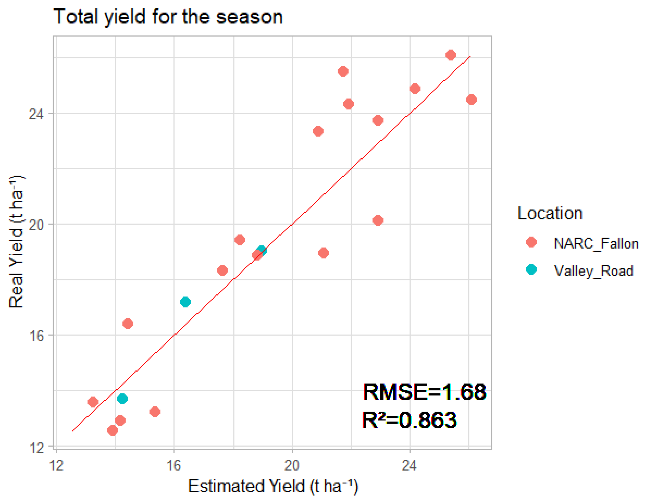
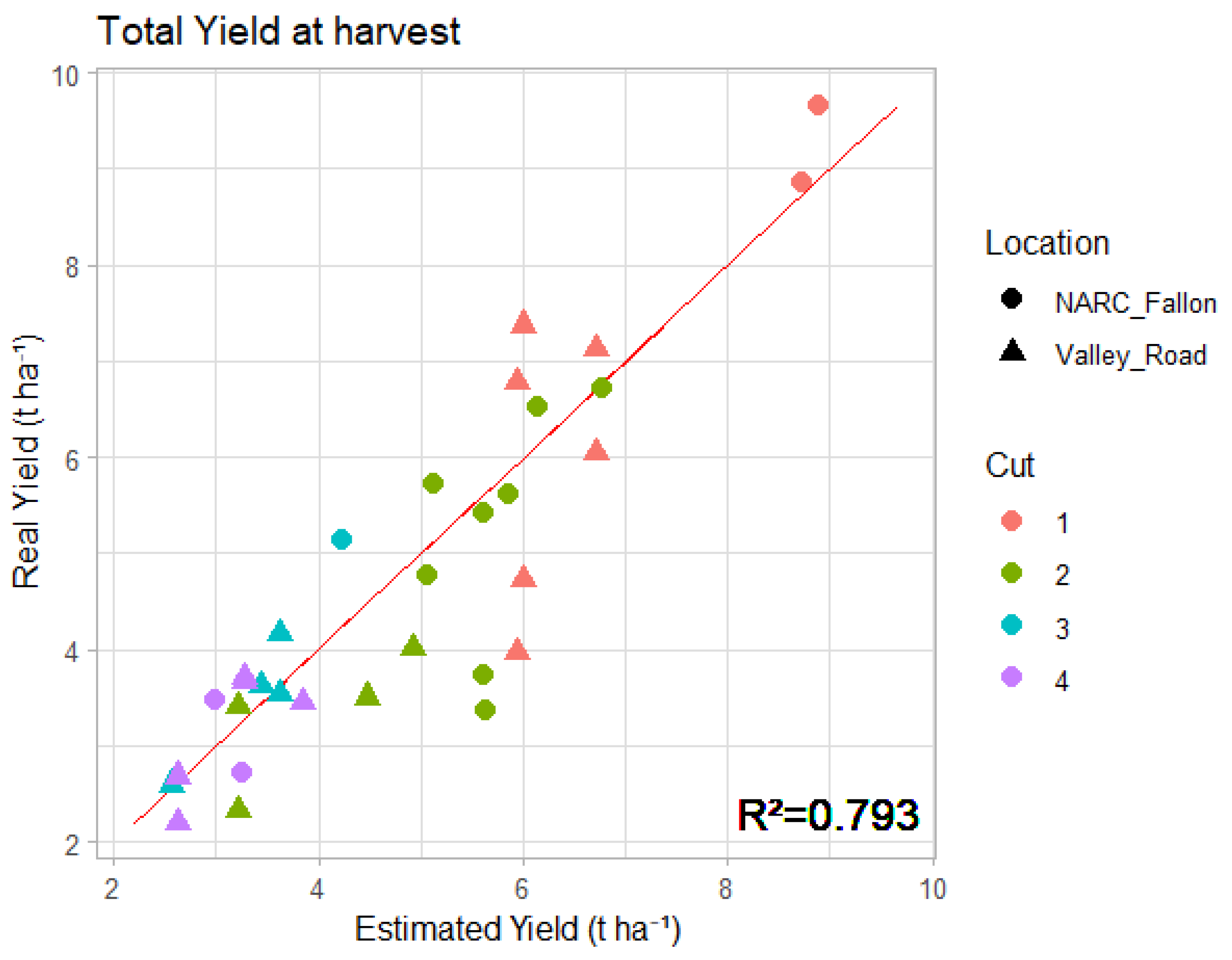
3.1. Linear Regression Model

The final LR model is represented by Equation (2), where “:” indicates an interaction term and “*” indicates an interaction term plus the interacting variables themselves. This means that P h p p h and C u t are included only as their interaction but T x a 30 and T x b 5 are included as their interaction and as independent variables too. Thus, the term P h p c h : C u t in Equation (2) is equal to i = 1 4 P h p c h C u t   i , where P h p c h C u t   i is the photoperiod for the i-th cut of the season; the term T x a 30 T x b 5 is equal to T x a 30 × T x b 5 + T x a 30 + T x b 5 . When the coefficients in Table 2 are included in Equation (2), the final LR model is presented in Equation (3). The response variable had to be log-transformed to fit the LR model’s assumptions. It should be noted that all the variables in Equation (2) except C u t were standardized, and that Cut is a categorical variable. The final LR model achieved an R2 of 0.948 for log Δ Y i e l d ¯ , 0.904 for Δ Y i e l d ¯ , and 0.854 for Y i e l d estimation. Figure 2 shows the yield values estimated using the model against observed yield values for both log Δ Y i e l d ¯ (a) and Y i e l d (b).
log Δ Y i e l d ¯ = P h p c h : C u t + W a t e r + W i n d + T x a 30 x b 5
log Δ Y i e l d ¯ = 3.207 0.482 P h p c h C u t 1 + 0.358 P h p c h C u t 2 + 0.015 P h p c h C u t 3 + 0.021 P h p c h C u t 4 + 0.313 W a t e r 0.161 W i n d 0.842 ( T x a 30 × T x b 5 ) 0.396 T x a 30 1.261 T x b 5
It can be said from Figure 2 that the model captures the variability of the response variable. The resulting coefficients of the model are shown in Table 1. All the coefficients are statistically significant (p < 0.05) except for P h p c h in the third and fourth harvests.
As expected, W a t e r has a positive effect on the yield. The linear response of the yield of herbaceous crops to water consumption has been widely reported in the literature [27]. W i n d exhibits a negative effect on the yield. Wind has been shown to increase evapotranspiration in highly advective arid and semi-arid regions [28,29]. Wind not only increases evapotranspiration rates but concomitantly increases soil salinity due to the accumulation of water-soluble salts on the soil surface after evaporative losses in arid and semi-arid environments [30]. This increase in salinity has a negative impact on plant growth and, ultimately, crop yield and may have been a contributing factor in this case [31]. Furthermore, wind has been reported to be an important factor in the spread of diseases in alfalfa crops, and those diseases can have a negative impact on the yield [32].
The temperature coefficients in the LR model had the highest values among all indicators (Table 2), which suggests that temperature has the greatest effect on the yield model. Figure 3 depicts the interaction effect of T x a 30 and T x b 5 . It suggests that the effect of extreme high temperatures is even higher when extremely low temperatures have occurred during the same YFP. Extreme temperatures lead to stress in the crop, which reflects a decrease in the yield [33,34].
The effect of low temperatures is also related to the dormant season. Dormant season in northern Nevada commonly lasts up to 6 months. During the dormant season, the crop is the most exposed to extreme low temperatures. In northern Nevada, this period accounts for approximately 28% of the yield for the first harvest [35]. Such a low yield accumulation rate during the dormant season might be driving the model to consider low temperatures as an important variable.
The photoperiod affects the yield accumulation rate by driving biomass partitioning. When the photoperiod starts to decrease, the crop starts to allocate its assimilates to the roots to have enough reserves for the dormant season [22]. It can be noticed that the effect of the photoperiod is the highest for the second harvest (Table 2). Usually, the second harvest occurs during summer, i.e., when the photoperiod is at its peak. According to the LR coefficients shown in Table 2, yield accumulation decreases with the length of the day during the harvests for the first cut, which is the opposite of the second harvest.
A possible explanation for the contrasting trend in the second harvest compared to the first is the combined effects of the increased intensity and duration of solar radiation and heat accumulation (growing degree days) during the period of the second harvest (longer days) relative to the first (shorter days). These aforementioned environmental factors are integral across the cycle of crop growth and development and, ultimately, for the yield of the crop, especially in cases where water or other production inputs (e.g., nutrients) are not a limiting factor [36,37].
A comparison of the observed yield against the estimated yield for Valley Road can be found in Figure 4. The LR model shows a good response to the variability in water. The LR model also showed its capability of capturing the response of the yield to different irrigation treatments. An alfalfa hay yield model capable of capturing the response of the crop to water can be used to analyze the effects of multiple irrigation management strategies on yield. Such a model can be incorporated into Decision Support Systems to improve the irrigation management of alfalfa.
Figure 5 shows the estimated and observed total seasonal yield for Fallon and Valley Road. With an R2 of 0.863, it can be noted that the model generalizes the seasonal yield well. The Root Mean Squared Error for the estimated seasonal yield was 1.68 t ha−1. This value has to be considered as the mean error of the LR model for the seasonal yield prediction.

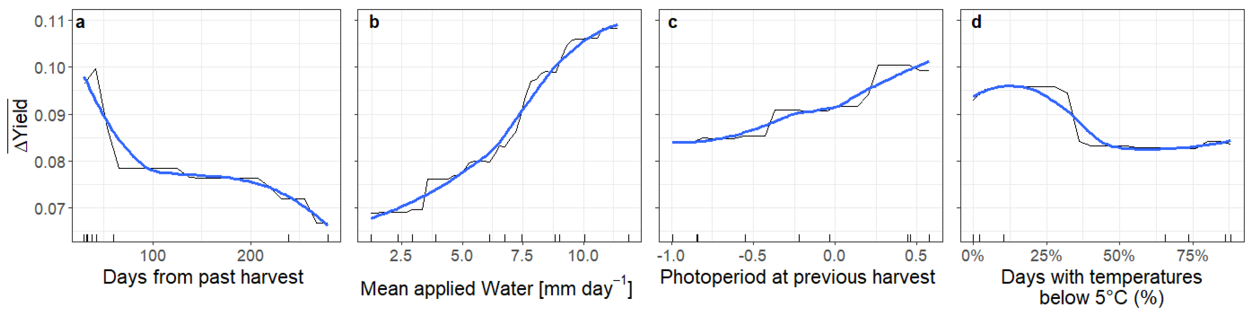
3.2. Random Forest Model

The resulting RF model has five variables as its predictor variables. In order of importance, the predictor variables of the RF model are D L H , W a t e r , P h p p h , and C u t , T n b 5 . R2 for the estimation of Δ Y i e l d ¯ for the RF model was 0.897 for the training dataset and 0.861 for the testing dataset. R2 for the estimation of Y i e l d was 0.793 (Figure 6). The presence of similar metrics on the training and testing datasets is an indicator of the capacity of the generalization of the model. Based on the R2, the RF model did not outperform the accuracy of the simpler LR model. Furthermore, when calculating R2 for Valley Road (2021 season) and NARC (1974–1981 season), separately, we obtained values of 0.738 and 0.789, respectively. These values show that the model did not overfit towards the most abundant season in the dataset (2021).
Figure 7 shows the partial dependency plots (PDPs) for the continuous predictor variables of the RF model. The PDPs showed the effect of the variation of a single variable while the outstanding variables remained constant in the model. The behavior of D L H (Figure 7a) is highly related to the dormant season. The first harvests are more influenced by D L H than the latter harvests; therefore, it is expected to have lower yield accumulation rates as the days since the past harvest increase.
The response of alfalfa hay yield to water (Figure 7b) exhibits a nearly logistic behavior. It is reasonable to expect this shape from this predictor variable since there will be some point at which the positive effect of the applied water on the yield will be minimum or null. The photoperiod shows a linear behavior; therefore, it does not reach a constant value within the defined range (Figure 7c), which suggests that the yield would continue increasing as the length of the day increases if there was no other limiting factor.
The occurrence of extremely low temperatures (Figure 7d) follows the same trend as in the LR model, even though the shape is not linear. Like D L H , the behavior of this curve is highly influenced by the dormant season (winter). Overall, the curve suggests a constant yield decrease when the percentage of days within the YFP with temperatures below 5 °C is over 50%.
The relative importance of the most relevant predictor variables can be assessed from the range of the y-axis in the partial dependency plots. Taking that into consideration, W a t e r and DLH could be the predictor variables with the highest effect on alfalfa hay yield. However, based on the slope of the curves, one can tell that the photoperiod (DLH) and temperature ( T n b 5 ) can have a greater effect within a very short range of their values.
It must be said that other variables are relevant for the estimation of alfalfa hay yield. For instance, radiation is expected to have a significant importance on the yield formation process. However, as the data were obtained from irrigated alfalfa plots, the water consumption is proportional to the crop evapotranspiration, and, thus, it is also proportional to the radiation amount.
Overall, both models (RF and LR) estimated alfalfa hay yield for two locations in northern Nevada with enough accuracy to be used to analyze the effects of different irrigation management scenarios on yield. The exposed relationship between weather, irrigation, and yield is well established and supported by prior physiological knowledge of the crop [27]. Even though the LR model showed the best performance, the weather–water–yield relationship might exhibit non-linear relationships under non-conventional irrigation management strategies, such as regulated deficit irrigation [38], where deficit irrigation is practiced at stages when the crop is less sensitive to water stress and avoided at stages when the crop is more sensitive to water stress. For this reason, it is important to advance our understanding of this relationship using non-linear models. The analysis performed in this work should be replicated, including more samples and exploring different non-linear models.

4. Conclusions

Linear models are good approaches with which to understand and explain yield accumulation in an irrigated alfalfa crop in northern Nevada. The LR model achieved an R2 of 0.854 and the RF model an R2 of 0.793 for the prediction of yield. Both water and the incidence of extreme temperatures are the most important weather features for the alfalfa yield accumulation process observed in northern Nevada. Having an indicator of the dormant season is important when modeling the alfalfa crop yield.
A linear model can capture and generalize the effect of water on the alfalfa crop; therefore, it is a good model to consider for a decision support system that assists the irrigation management of alfalfa.
Further work is recommended to perform a similar analysis that includes additional data, as well as to more accurately represent the effect of the dormant season. This will lead to a better understanding of the effect of temperature and dormancy on the alfalfa crop yield. This could also help to identify responses in other variables.
The performed analysis, by itself, is not enough to establish a direct causal relationship between the studied variables and the crop yield. Physiological studies are necessary to support those relations that, so far, are only suggested by data and models.

Author Contributions

Conceptualization, D.Q. and M.A.A.; methodology, D.Q.; software, D.Q.; validation, D.Q.; collection of experimental data, D.Q., U.C. and M.A.A.; formal analysis, D.Q.; writing—original draft preparation, D.Q.; writing—review and editing, D.Q., M.A.A., U.C. and J.K.Q.S.; supervision, M.A.A. and J.K.Q.S.; project administration, M.A.A.; funding acquisition, M.A.A. All authors have read and agreed to the published version of the manuscript.

Funding

This research was funded by the University of Nevada, Reno, Office of Research and Innovation and the Nevada Agricultural Experiment Station (NAES) of the College of Agriculture, Biotechnology & Natural Resources, University of Nevada, Reno. This research was supported in part by the U.S. Department of Agriculture, National Institute of Food and Agriculture, DSFAS program, under Award No. 2023-67022-40041.

Data Availability Statement

The data presented in this study are available on request from the corresponding author.

Acknowledgments

The authors acknowledge the dedicated work performed by Scott Huer, Field Research Coordinator of the University of Nevada, Reno, Nevada Agricultural Experiment Station.

Conflicts of Interest

The authors declare no conflict of interest.

References

  1. Rumberg, S. Nevada Agricultural Statistics Annual Bulletin 2016 Crop Year. 2016. Available online: https://www.nass.usda.gov/Statistics_by_State/Nevada/Publications/Annual_Statistical_Bulletin/2010s/NVANNBUL_update_Dec14.pdf (accessed on 13 May 2022).
  2. Graeff, S.; Link, J.; Binder, J.; Claupei, W. Crop Models as Decision Support Systems in Crop Production. In Crop Production Technologies; InTech: Rijeka, Croatia, 2012. [Google Scholar] [CrossRef]
  3. Teh, C.B.S. Introduction to Mathematical Modeling of Crop Growth: How the Equations are Derived and Assembled into a Computer Model; Brown Walker Press: Irvine, CA, USA, 2006. [Google Scholar]
  4. Boogaard, H.L.; De Wit, A.J.W.; Te Roller, J.A.; Van Diepen, C.A. Wofost Control Centre 2.1; User’s Guide for the Wofost Control Centre 2.1 and the Crop Growth Simulation Model Wofost 7.1.7; Alterra, Wageningen University & Research Centre: Wageningen, The Netherlands, 2014. [Google Scholar]
  5. Shi, W.; Tao, F.; Zhang, Z. A review on statistical models for identifying climate contributions to crop yields. J. Geogr. Sci. 2013, 23, 567–576. [Google Scholar] [CrossRef]
  6. Mishra, S.; Mishra, D.; Santra, G.H. Applications of Machine Learning Techniques in Agricultural Crop Production: A Review Paper. Indian J. Sci. Technol. 2016, 9, 1–4. [Google Scholar] [CrossRef]
  7. Sharma, A.; Jain, A.; Gupta, P.; Chowdary, V. Machine Learning Applications for Precision Agriculture: A Comprehensive Review. IEEE Access 2021, 9, 4843–4873. [Google Scholar] [CrossRef]
  8. Everingham, Y.; Sexton, J.; Skocaj, D.; Inman-Bamber, G. Accurate prediction of sugarcane yield using a random forest algorithm. Agron. Sustain. Dev. 2016, 36, 1–9. [Google Scholar] [CrossRef]
  9. Ghazvinei, P.T.; Darvishi, H.H.; Mosavi, A.; Yusof, K.; Bin, W.; Alizamir, M.; Shamshirband, S.; Chau, K. Sugarcane growth prediction based on meteorological parameters using extreme learning machine and artificial neural network. Eng. Appl. Comput. Fluid Mech. 2018, 12, 738–749. [Google Scholar] [CrossRef]
  10. Nantasaksiri, K.; Chareon-amornkitt, P. Comparison of Multiple Regression Analyses for Napier Grass Dry Matter Yield Prediction. JCREN 2015. Available online: https://www.researchgate.net/profile/Patcharawat-Charoen-Amornkitt/publication/287992611_Comparison_of_Multiple_Regression_Analyses_for_Napier_Grass_Dry_Matter_Yield_Prediction/links/567b5cd808aebccc4dfd9411/Comparison-of-Multiple-Regression-Analyses-for-Napier-Grass-Dry-Matter-Yield-Prediction.pdf (accessed on 16 May 2022).
  11. Whitmire, C.D.; Vance, J.M.; Rasheed, H.K.; Missaoui, A.; Rasheed, K.M.; Maier, F.W. Using Machine Learning and Feature Selection for Alfalfa Yield Prediction. AI 2021, 2, 71–88. [Google Scholar] [CrossRef]
  12. Moraffah, R.; Karami, M.; Guo, R.; Raglin, A.; Liu, H. Causal Interpretability for Machine Learning—Problems, Methods and Evaluation. ACM SIGKDD Explor. Newsl. 2020, 22, 18–33. [Google Scholar] [CrossRef]
  13. Qi, Y. Random Forest for Bioinformatics. Ensemble Mach. Learn. 2012, 307–323. [Google Scholar] [CrossRef]
  14. Luan, J.; Zhang, C.; Xu, B.; Xue, Y.; Ren, Y. The predictive performances of random forest models with limited sample size and different species traits. Fish. Res. 2020, 227, 105534. [Google Scholar] [CrossRef]
  15. Rashedi, N. Evapotranspiration Crop Coefficients for Alfalfa at Fallon, Nevada; University of Nevada: Reno, Nevada, 1983. [Google Scholar]
  16. Cholula, U.; Quintero-Puentes, D.; Andrade, M.; Solomon, J. Effects of Deficit Irrigation on Yield and Water Productivity of Alfalfa in Northern Nevada. In Proceedings of the 2022 ASABE Annual International Meeting, Houston, TX, USA, 17–20 July 2022. [Google Scholar]
  17. NOAA. Climate Data Online: Web Services Documentation. Available online: https://www.ncdc.noaa.gov/cdo-web/webservices/v2 (accessed on 13 October 2021).
  18. WRCC. RAWS USA Climate Archive. Available online: Https://Raws.Dri.Edu/ (accessed on 13 October 2021).
  19. World Meteorological Organization. Guidelines on Surface Station Data Quality Control and Quality Assurance for Climate Applications. WMO-No. 1269. 2021. Available online: https://library.wmo.int/records/item/57727-guidelines-on-surface-station-data-quality-control-and-quality-assurance-for-climate-applications (accessed on 18 October 2023).
  20. NOAA/OAR/ESRL. 20th Century Reanalysis Data. Available online: https://www.psl.noaa.gov/data/gridded/data.20thC_ReanV3.html. (accessed on 13 October 2021).
  21. Moot, D.J.; Yang, X.; Ta, H.T.; Brown, H.E.; Teixeira, E.I.; Sim, R.E.; Mills, A. Simplified methods for on-farm prediction of yield potential of grazed lucerne crops in New Zealand. New Zealand J. Agric. Res. 2021, 65, 252–270. [Google Scholar] [CrossRef]
  22. Kallenbach, R.L.; Nelson, C.J.; Coutts, J.H. Yield, Quality, and Persistence of Grazing- and Hay-Type Alfalfa under Three Harvest Frequencies. Agron. J. 2002, 94, 1094–1103. [Google Scholar] [CrossRef]
  23. R Core Team. R: A Language and Environment for Statistical Computing. 2021. Available online: https://www.r-project.org/ (accessed on 13 October 2021).
  24. Liaw, A.; Wiener, M. Classification and Regression by randomForest. R News 2002, 2, 18–22. Available online: https://cran.r-project.org/doc/Rnews/ (accessed on 18 October 2023).
  25. Greenwell, B.M. pdp: An R Package for Constructing Partial Dependence Plots. R.J. 2017, 9, 421–436. Available online: https://journal.r-project.org/archive/2017/RJ-2017-016/index.html (accessed on 18 October 2023). [CrossRef]
  26. Probst, P.; Wright, M.; Boulesteix, A.L. Hyperparameters and tuning strategies for random forest. WIREs Data Mining Knowl. Discov. 2019, 9, e1301. [Google Scholar] [CrossRef]
  27. Steduto, P.; Hsiao, T.C.; Fereres, E.; Raes, D. Crop Yield Response To Water. Food and agriculture organization of the united nations. 2012. Available online: https://www.researchgate.net/profile/Nageswara-Rao-V/publication/236894273_Suhas_P_Wani_Rossella_Albrizio_V_Nageswara_Rao_2012_Sorghum_In_Crop_Yield_response_to_Water_FAO_Irrigation_and_Drainage_Paper_66_Eds_Pasquale_Steduto_Theodore_C_Hsiao_Elias_Fereres_and_Dirk_RaesPages_/links/0deec51a01ddf96cca000000/Suhas-P-Wani-Rossella-Albrizio-V-Nageswara-Rao-2012-Sorghum-In-Crop-Yield-response-to-Water-FAO-Irrigation-and-Drainage-Paper-66-Eds-Pasquale-Steduto-Theodore-C-Hsiao-Elias-Fereres-and-Dirk-RaesP.pdf (accessed on 13 October 2021).
  28. Berengena, J.; Gavilán, P. Reference Evapotranspiration Estimation in a Highly Advective Semiarid Environment. J. Irrig. Drain. Eng. 2005, 131, 147–163. [Google Scholar] [CrossRef]
  29. Evett, S.R.; Howell, T.A.; Schneider, A.D.; Copeland, K.S.; Dusek, D.A.; Brauer, D.K.; Tolk, J.A.; Marek, G.W.; Thomas, M.; Gowda, P.H. The Bushland weighing lysimeters: A quarter century of crop ET investigations to advance sustainable irrigation 7004(November). Trans. ASABE. 2016, 59, 163–179. [Google Scholar]
  30. Stavi, I.; Thevs, N.; Priori, S. Soil salinity and Sodicity in drylands: A review of causes, effects, monitoring, and restoration measures. Front. Environ. Sci. 2021, 9, 330. [Google Scholar] [CrossRef]
  31. Abuelgasim, A.; Ammad, R. Mapping soil salinity in arid and semi-arid regions using Landsat 8 Oli Satellite Data. Remote Sens. Appl. Soc. Environ. 2019, 13, 415–425. [Google Scholar] [CrossRef]
  32. Claflin, L.E.; Stuteville, D.L.; Armbrust, D.V. Wind-Blown Soil in the Epidemiology of Bacterial Leaf Spot of Alfalfa and Common Blight of Bean. Phytopathology 1973, 63, 1417–1419. [Google Scholar] [CrossRef]
  33. Wassie, M.; Zhang, W.; Zhang, Q.; Ji, K.; Chen, L. Effect of Heat Stress on Growth and Physiological Traits of Alfalfa (Medicago sativa L.) and a Comprehensive Evaluation for Heat Tolerance. Agronomy 2019, 9, 597. [Google Scholar] [CrossRef]
  34. Zhu, R.Y.; Lei, J.Y.; Qu, L.; Chen, Y.; Jin, J. Metabolic responses of alfalfa (Medicago Sativa L.) leaves to low and high temperature induced stresses. Afr. J. Biotechnol. 2013, 10, 1117–1124. [Google Scholar]
  35. Goodrich, M. Dormant Season Evapotranspiration in Alfalfa; University of Nevada, Reno: Reno, Nevada, 1986. [Google Scholar]
  36. Villegas, D.; Alfaro, C.; Ammar, K.; Cátedra, M.M.; Crossa, J.; García del Moral, L.F.; Royo, C. Daylength, temperature and solar radiation effects on the phenology and yield formation of spring durum wheat. J. Agron. Crop Sci. 2015, 202, 203–216. [Google Scholar] [CrossRef]
  37. Ferrante, A.; Mariani, L. Agronomic management for enhancing plant tolerance to abiotic stresses: High and low values of temperature, light intensity, and relative humidity. Horticulturae 2018, 4, 21. [Google Scholar] [CrossRef]
  38. Liu, M.; Wang, Z.; Mu, L.; Xu, R.; Yang, H. Effect of regulated deficit irrigation on alfalfa performance under two irrigation systems in the inland arid area of midwestern China. Agric. Water Manag. 2021, 248, 106764. [Google Scholar] [CrossRef]
Figure 1. (a) Locations of Valley Road Field Laboratory (VRFL) and Nevada Agricultural Research Station (NARS), where the data used to train the linear regression (LR) and random forest (RF) models were collected. Climographs for both locations were generated using weather data for the study period in each location: 2020–2021 for VRFL (b) and 1973–1981 for NARS (c).
Agriengineering 05 00119 g001
Figure 2. Estimated yield values obtained by the LR model vs. observed yield: (a) Fitted model using the log of the mean daily increment in yield. (b) Yield at harvest calculated using the fitted model. Cut label corresponds to different harvests throughout the season. Red line is the 1:1 line.
Agriengineering 05 00119 g002
Figure 3. Effect of the occurrence of extreme high temperatures interacting with the occurrence of extreme low temperatures through the yield formation period. The effect of the occurrence of extreme high temperatures increases as the occurrence of extreme low temperatures increases.
Agriengineering 05 00119 g003
Figure 4. The estimated yield obtained from the LR model vs. observed yield for Valley Road. Cut label corresponds to different harvests. The treatment label matches different irrigation treatments (100%, 80%, and 60% of soil water depletion replenishment to field capacity). Red line is the 1:1 line.
Agriengineering 05 00119 g004
Figure 5. Observed yield vs. estimated yield obtained using the LR model for the entire season for both locations. Red line is the 1:1 line.
Agriengineering 05 00119 g005
Figure 6. Observed yield vs. estimated yield obtained using the RF model for every cut in both locations. Red line is the 1:1 line.
Agriengineering 05 00119 g006
Figure 7. Partial dependency plots for four of the most relevant predictor variables identified for the RF model: (a) Days from past harvest; (b) Mean applied Water; (c) Photoperiod at previous harvest; (d) Days with temperatures below 5 °C. Black line indicates the actual RF output. The blue line is a smooth line fitted to the RF output.
Agriengineering 05 00119 g007
Table 1. Weather and water management indicators used in the analysis.
IndicatorDescription
P h p c h Photoperiod of current harvest = C o s π 0.94 + J 183 , where J is the Julian day of the current harvest.
P h p p h Photoperiod of previous harvest = C o s π 0.94 + J 183 , where J is the Julian day of the previous harvest.
W a t e r Average of the total rain and irrigation input during the yield formation period (YFP).
S R a d Daily mean solar radiation during YFP.
G D D Total growing degree days during YFP.
W i n d Average daily wind speed during YFP.
T n b 5 Fraction of days during YFP with minimum daily temperature below 5 °C.
T x b 5 Fraction of days during YFP with maximum daily temperature below 5 °C.
T n a 20 Fraction of days during YFP with minimum daily temperatures above 20 °C.
T x a 30 Fraction of days during YFP with maximum daily temperatures above 30 °C.
D L H Days since the last harvest.
C u t Number of harvests (cut) in that season. E.g., 1 for the first harvest, 2 for the second, and so on.
Table 2. Resulting coefficients for the LR model.
CoefficientEstimatePr (<|t|)
I n t e r c e p t −3.2070.000
W a t e r +0.3130.000
W i n d −0.1610.000
T x a 30 −0.3960.011
T x b 5 −1.2610.001
P h p c h : C u t [ 1 ] −0.4820.034
P h p c h : C u t [ 2 ] +0.3580.000
P h p c h : C u t [ 3 ] +0.0150.858
P h p c h : C u t [ 4 ] +0.0210.477
T x a 30 : T x b 5 −0.8420.001
Disclaimer/Publisher’s Note: The statements, opinions and data contained in all publications are solely those of the individual author(s) and contributor(s) and not of MDPI and/or the editor(s). MDPI and/or the editor(s) disclaim responsibility for any injury to people or property resulting from any ideas, methods, instructions or products referred to in the content.

