Crop Yield Estimation Using Sentinel-3 SLSTR, Soil Data, and Topographic Features Combined with Machine Learning Modeling: A Case Study of Nepal

Abstract

Effective crop monitoring and accurate yield estimation are fundamental for informed decision-making in agricultural management. In this context, the present research focuses on estimating wheat yield in Nepal at the district level by combining Sentinel-3 SLSTR imagery with soil data and topographic features. Due to Nepal’s high-relief terrain, its districts exhibit diverse geographic and soil properties, leading to a wide range of yields, which poses challenges for modeling efforts. In light of this, we evaluated the performance of two machine learning algorithms, namely, the gradient boosting machine (GBM) and the extreme gradient boosting (XGBoost). The results demonstrated the superiority of the XGBoost-based model, achieving a determination coefficient (R²) of 0.89 and an RMSE of 0.3 t/ha for training, with an R² of 0.61 and an RMSE of 0.42 t/ha for testing. The calibrated model improved the overall accuracy of yield estimates by up to 10% compared to GBM. Notably, total nitrogen content, slope, total column water vapor (TCWV), organic matter, and fractional vegetation cover (FVC) significantly influenced the predicted values. This study highlights the effectiveness of combining multi-source data and Sentinel-3 SLSTR, particularly proposing XGBoost as an alternative tool for accurately estimating yield at lower costs. Consequently, the findings suggest comprehensive and robust estimation models for spatially explicit yield forecasting and near-future yield projection using satellite data acquired two months before harvest. Future work can focus on assessing the suitability of agronomic practices in the region, thereby contributing to the early detection of yield anomalies and ensuring food security at the national level.

1. Introduction

Recognizing the global significance of food security vis-à-vis sustainable agriculture, the United Nations, through its Sustainable Development Goals (SDG2: Zero Hunger and SDG15: Life on Land), has called upon states to align their development agendas towards the promotion of sustainable food production systems and the implementation of suitable agronomic practices to enhance agricultural productivity. One key aspect in achieving these goals is crop yield estimation, which can help identify and characterize long-standing and persistent underperforming farming regions [1,2] toward ensuring food security for present and future generations.

The escalating demand for food at an unprecedented rate emphasizes the importance of timely information on crop growth stages and maturity for effective decision-making, emergency response mechanisms, and efficient monitoring of food production [3]. As a result, various approaches have been employed to model crop yield, including field surveys, expert assessments, farm reports, and forecasting models [4,5,6]. In recent years, integrating remote sensing and machine learning tools has sparked a fundamental shift in sustainable agriculture. Notably, crop yield estimation has become one of its main applications, particularly in precision agriculture [7,8], offering valuable insights for local and regional decision-making regarding agronomic practices and parametric insurance, ultimately fostering local economies and ensuring food security [9].

Sustainable agriculture has undergone a tremendous change with the emergence of remote sensing and machine learning tools [10,11]. By leveraging spectral information derived from multispectral data [12,13,14,15] and incorporating geospatial data on surface properties retrieved from synthetic aperture radar (SAR) data [16,17], along with other data sources like climatic and phenological data [18,19,20], researchers have made significant progress in modeling agricultural productivity and monitoring crop growth. For this purpose, various prediction models have been commonly employed for yield estimation, including random forests [21,22], neural networks [23], gradient-boosting trees [24], and linear regression analysis [25], among other tools that involve deep learning and artificial intelligence [26,27]. Such alternative approaches hold great promise for decision-makers and farmers, enabling installation of sustainable farming systems and facilitating effective surveying practices. For instance, Wolanin et al. [28] have estimated a crop yield variation in the Indian Wheat Belt using deep learning and time-series analysis based on vegetation cover and meteorological data. Their findings demonstrated that deep neural networks outperformed other algorithms, highlighting the significance of growing season length, temperature, and radiation conditions as key parameters in crop yield assessment. In Hungary, Ferencz et al. [29] employed Landsat Thematic Mapper™ data to develop a novel vegetation index known as the General Yield Unified Reference Index (GYURI). This index was derived by fitting a double-Gaussian curve to the National Oceanic and Atmospheric Administration (NOAA) Advanced Very High-Resolution Radiometer (AVHRR) data, specifically during the vegetation period. Their study focused on assessing wheat and corn yields over a three-year period while determining the average yield per county. The results revealed the potential of remote sensing data for yield estimation, with a coefficient of determination (R²) ranging from 0.75 to 0.93 between the GYURI index and corn yield. In Spain, Franch et al. [30] have successfully estimated rice yield by combining Sentinel-1 SAR and Sentinel-2 MSI data through regression analysis. They demonstrated that the highest correlation between satellite data and crop yield could be observed three months before harvest, with an R² ranging from 0.72 to 0.92. This study uncovered a strong association between rice yield and spectral information obtained from spaceborne remote sensing platforms, providing valuable insights into vulnerable areas in the coastal wetland Albufera, where farmers’ interventions can be optimized. In Kenya, Adebayo et al. [31] evaluated the predictive performance of random forest, support vector machine, and feedforward neural network models for maize yield estimation based on Sentinel-1 SAR and Sentinel-2 MSI data. The research found that the random forest-based model yielded the best performance among other machine learning models, explaining 76% of data variance. This finding serves as a reference for selecting appropriate algorithms in future crop yield prediction studies.

Nevertheless, the application of Sentinel-3 data in crop yield assessment has been relatively limited in the existing research. Notably, Bojanowski et al. [32] have used Sentinel-3 OLCI and SLSTR data in combination with MODIS and ERA5 data to establish a forecasting model of corn and wheat yields between 2000 and 2019 in Poland. This study demonstrated promising outcomes, with root mean square errors (RMSE) ranging from 8.15% to 13%, highlighting the potential application of Sentinel-3 data, despite their coarse resolution, in accurately estimating yield at a regional scale. However, additional investigation on the capabilities and constraints of Sentinel-3 data for crop yield prediction is justified, given the limited research conducted so far.

In this context, the present work aims to estimate the average Nepalese wheat crop yield per district by leveraging advanced machine learning tools in combination with remote sensing data retrieved from Sentinel-3 SLSTR. To achieve this, we have integrated other data types, including topographic covariates and soil information, which substantially influence agricultural productivity. By adopting a multidimensional approach, this study aims to provide practical insights into developing an effective and timely methodology for estimating wheat yield at the country scale. This work will assist in addressing challenges associated with food security by enhancing our understanding of crop production dynamics and optimizing agricultural practices through yield estimation in the early stages.

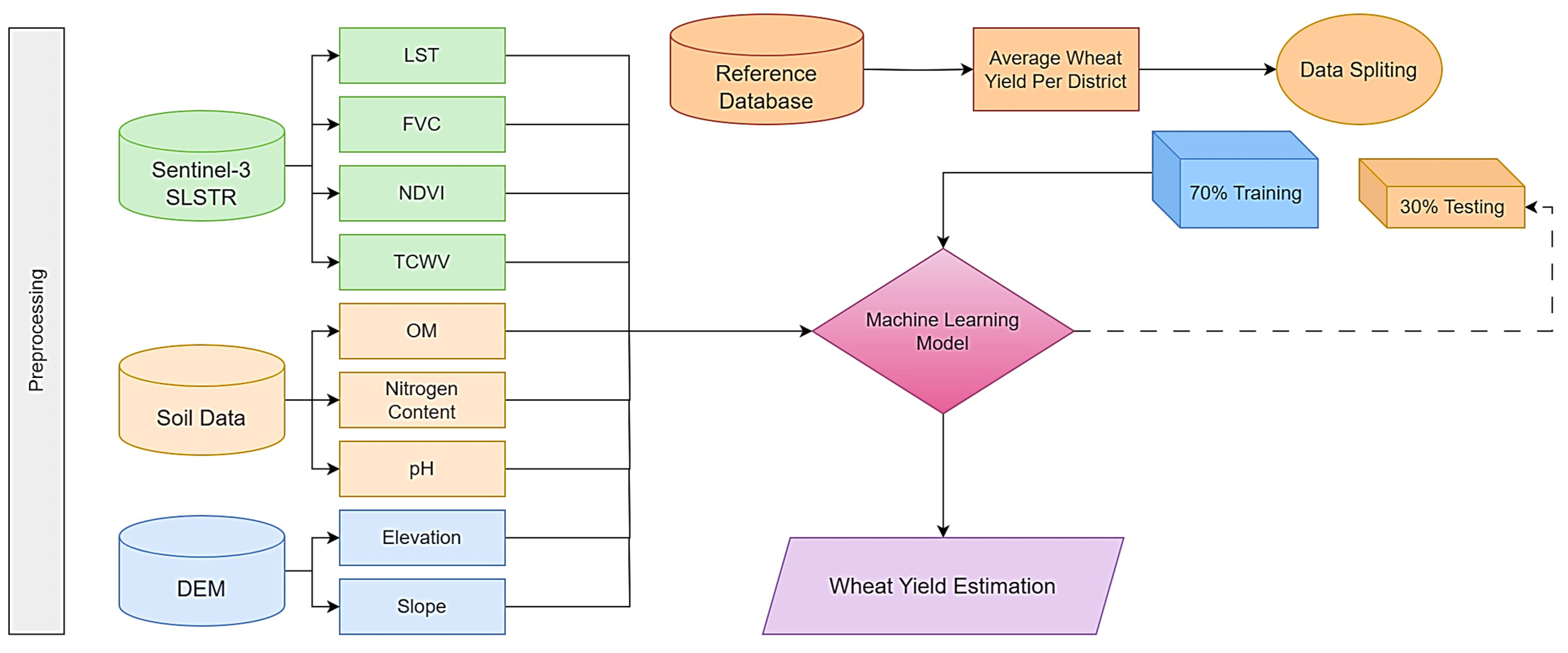
2. Materials and Methods

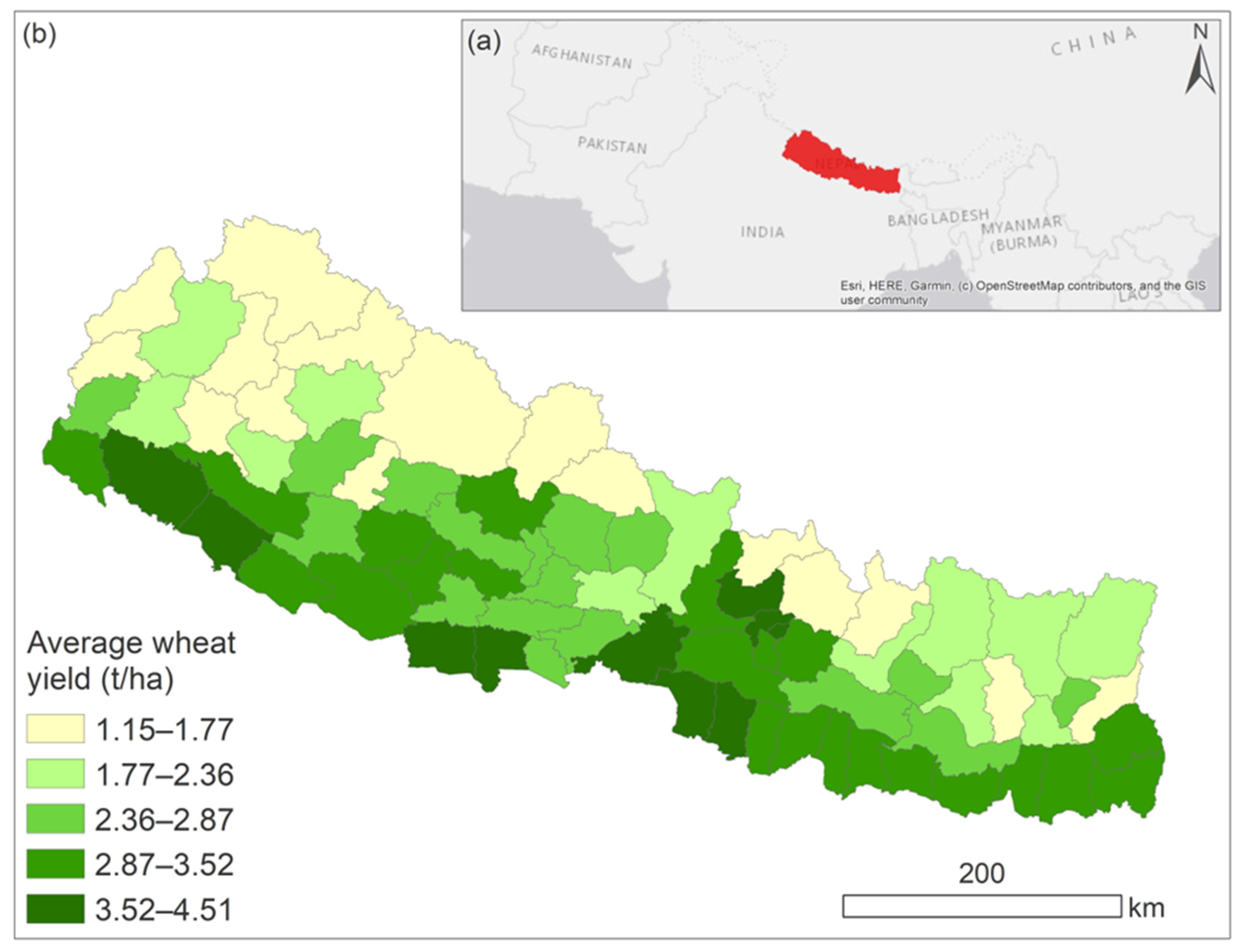
2.1. Study Area and Reference Data

Nepal is situated in Southeast Asia, spanning between latitudes 26° 22′ N and 30° 27′ N and longitudes 80° 00′ E and 88° 00′ E (Figure 1). With a surface area of approximately 147,516 km² [33], Nepal is divided into seven provinces and 77 districts, each owning distinct topographical features across their regions [34]. The country is characterized by five physiographic regions: Terai, Siwaliks, Middle Mountains, High Mountains, and High Himalayas, further divided into three zones: the Terai, the Hill, and the Himalayas [35]. These divisions provide valuable insights into the diverse topographic landscapes present within Nepal’s geographical boundaries. In addition, Nepal boasts a wide range of elevations, extending from 60 m above sea level to the world’s highest peak, Mount Everest, at 8850 m [36]. The climate is highly diverse due to its topographic complexity, categorized into four main types based on the Köppen climate classification: temperate (C), arid (B), cold (D), and polar (E) [37]. Nepal experiences four distinct seasons with varying weather patterns: the pre-monsoon season from March to May, the summer monsoon from June to September, the post-monsoon season from October to November, and the winter season from December to February. The mean precipitation is 1800 mm/year [38]. The average temperature exhibits seasonal fluctuations, with summer temperatures ranging between 20 °C and 35 °C, while winter temperatures range between 2 °C and 12 °C [39]. In the mountainous catchment areas, the mean evapotranspiration rate fluctuates between 1300 and 1400 mm per year [40].

As the distribution of soil types in Nepal is mainly influenced by its topography, inceptisols dominate the hilly zones and lower tropical mountain regions, while spodosols occupy the subalpine forest and alpine shrub areas [41]. On the other hand, land use and land cover have been primarily influenced by combined anthropogenic and natural processes, which have continuously changed in recent decades due to climate change [42]. Agriculturally, cereal production in Nepal has significantly contributed to food security, with rice, wheat, and maize being the three major crops jointly contributing to 30.92% of its GDP [43].

As one of the most economically disadvantaged countries in Asia, Nepal faces serious socioeconomic challenges that will profoundly impact its population of 30 million people [44]. A quarter of the Nepalese population lives in poverty, struggling to meet their basic needs and access essential services [45]. This pervasive poverty indicates the pressing need for sustainable development initiatives and targeted interventions to uplift the living standards of the affected communities. Moreover, with half of the country’s districts consistently confronting limited access to nutritious food sources, Nepal experiences yearly food deficits. This further amplifies the nation’s socioeconomic vulnerability and impedes progress toward achieving food security through initiatives on cropping system monitoring and yield estimation [46].

Reference data on average wheat yield in tons per hectare (t/ha) for 77 districts have been retrieved from the statistical information report number 2077/78 on Nepalese agriculture. This annual publication was prepared for the fiscal year 2020/21 and released by the Ministry of Agriculture and Livestock Development Planning in July 2022 [47]. The report provides updated data on diverse aspects of Nepal’s socioeconomic sectors, including crops, livestock, and fisheries, among other key inputs. The document offers detailed insights into the agricultural sector and its performance. For more information on the reference data, it can be retrieved from the Nepal in Data portal, available at https://nepalindata.com/resource/STATISTICAL-INFORMATION-ON-NEPALESE-AGRICULTURE-2077-78--2020-21/ accessed on 30 March 2023.

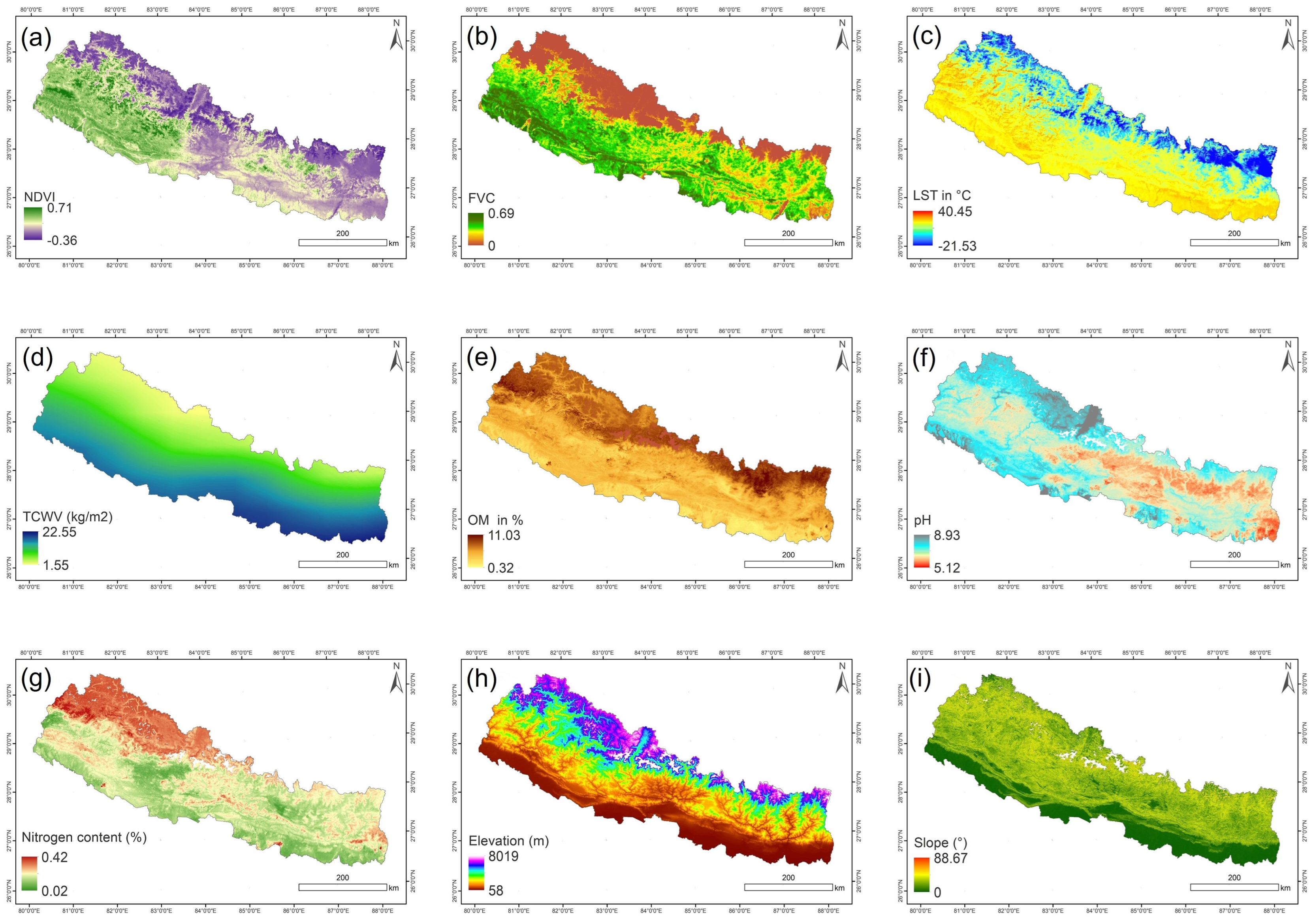
2.2. Remote Sensing Data and Other Features

The Sea and Land Surface Temperature Radiometer (SLSTR) is a dual-scan temperature radiometer selected for the ESA Sentinel-3 mission in low earth orbit as a part of the Copernicus Programme [48]. The instrument provides a wide range of applications related to earth observation, with a primary focus on sea surface temperature (SST) and land monitoring [49]. SLSTR products offer highly accurate global and regional measurements of sea and land surface temperature (SST and LST), supporting various environmental-related studies [50,51]. The mission delivers data with a high temporal resolution of less than half a day of revisit time. However, it features a moderately coarse spatial resolution, ranging from 500 m to 1 km. Such temporal and spatial properties make the data sufficiently intricate to be incorporated into various applications, encompassing factors such as soil moisture content, surface heterogeneity, and vegetation cover [52,53,54]. In the present study, we acquired the Sentinel-3 SLSTR Level 2 product sensed on 26 February 2021 and performed a co-registration and geometric correction. Following this, we extracted these key features: land surface temperature (LST), which was converted from kelvin to degrees Celsius (°C), total column water vapor (TCWV), normalized difference vegetation index (NDVI), and fractional vegetation cover (FVC). It is crucial to emphasize that our deliberate choice of acquiring data at the end of February aligns with the observations of the wheat growth season according to Nepal’s crop calendar (end of February to mid-March) [55], a time frame that was further confirmed by Sahbeni et al. [56].

For soil information, we retrieved reference maps on soil properties, including soil organic matter (SOM) (%), total nitrogen content (%), and pH from the National Soil Science Research Center (NARC) website, accessed at https://soil.narc.gov.np, accessed on 30 March 2023. These products have a spatial resolution of approximately 250 m. For topographic data, we acquired a Shuttle Radar Topography Mission (SRTM GL1) Global 30-m (SRTM_GL1) product, from which elevation (m) and slope (degrees) data were derived [57]. SRTM GL1 (30 m ellipsoidal) represents a version of the SRTM dataset that employs elevation values from WGS84 ellipsoidal height instead of the usual orthometric or geoid-referenced elevation. This dataset was generated by subtracting the EGM96 geoid model from the standard SRTM GL1 data, and it features a resolution of 1 arc-second (ca. 30 m at the Equator) [58]. The resulting covariates derived from Sentinel-3 SLSTR, soil maps, and SRTM DEM are presented in

Table 1. Variables used in the research and their descriptions.

Variable	Description
LST (°C)	Measurement of surface temperature inland
TCWV (kg/m2)	Quantification of the total water vapor in the atmosphere
NDVI	Indicator of vegetation density and health
FVC	Estimation of the proportion of land covered by vegetation
OM (%)	Percentage of organic matter in the soil
pH	Measurement of the acidity or alkalinity of the soil
Total nitrogen content (%)	Proportion of nitrogen content in the soil
Elevation (m)	Altitude above sea level at a specific location
Slope (degrees)	Inclination or gradient of the land surface

and Figure 2.

Following the reprojection of geospatial data to the Universal Transverse Mercator (UTM) coordinate system using the World Geodetic System (WGS) 1984 datum assigned to the North UTM Zone 44 and resampling them to a 30 m spatial resolution, we masked out non-cropland areas at the country level. For this step, we used the biome layer within the Sentinel-3 SLSTR data. This layer is a modified version of the GlobCover classification [59], re-gridded to 1/120° resolution. Thus, we focused on Class 11 and 20, which represent irrigated and rain-fed croplands, respectively [60]. By considering only these classes, we extracted cropland areas within the boundaries of Nepal. Subsequently, we derived the mean values per district from the resulting variables using the “zonal statistics as Table” tool in ESRI ArcMap^® 10.3. Once we compiled a comprehensive database containing nine independent variables and one dependent variable (average wheat yield per district), we imported it into RStudio. Then, we performed training, calibration, and testing of the machine learning models. Out of the 77 available observations, we allocated 70% of the data for training, while the remaining 30% were used for testing. Figure 3 provides a visual representation of the study’s flowchart, illustrating the sequential steps undertaken throughout the analysis.

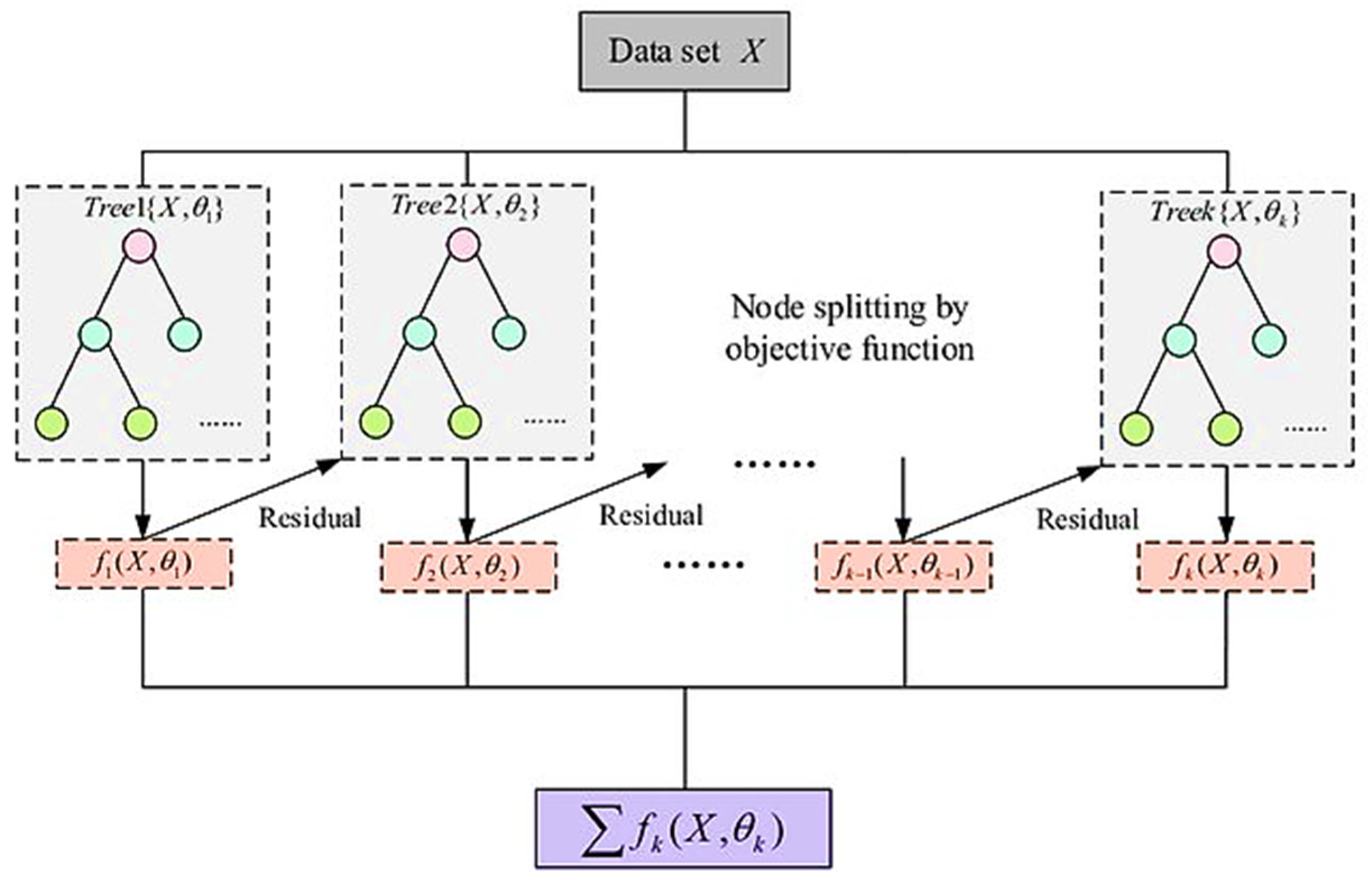
2.3. Gradient Boosting Machine (GBM) versus Extreme Gradient Boosting (XGBoost)

The gradient boosting machine (GBM) is a highly influential machine learning algorithm that has earned significant attention in diverse environmental applications, including agriculture [61], climatology [62], and soil studies [63]. GBM stands out as a robust tool due to its ability to leverage tree-like structures for decision-making [64]. Notably, its potential in crop yield estimation has been widely recognized and acknowledged by experts in the field [65]. One of the main advantages of GBM is its versatility, as it can be employed for both regression and classification tasks, enabling effective policy-making in various scenarios [66]. The ensemble learning algorithm sequentially builds upon weak trees, progressively enhancing the previous models’ performance. This iterative process creates powerful predictive models capable of delivering accurate estimates [67]. The reliability of GBM in fitting new trees and generating accurate predictions has been well-documented across different fields. For instance, it has been successfully implemented in actual evapotranspiration estimation, allowing a better understanding of short-term drought episodes associated with surface temperature and vegetation cover changes in Kenya [52]. Further, GBM has demonstrated its effectiveness in land cover and land use assessment, enabling more precise land surface mapping and monitoring [68]. It has also shown potential in water quality assessment, facilitating the prediction of water quality indices for monitoring purposes [69]. In this analysis, we used the “gbm” package in R Studio to implement this approach. Its fundamental concept, adopted by Friedman [70], is summarized by Algorithm 1.

Algorithm 1: Friedman’s gradient boost algorithm

Inputs:

Input data ${(\mathbf{x},\mathbf{y})}_{\mathbf{i}=1}^{\mathbf{N}}$ Number of iterations M Choice of the loss-function $\mathsf{\psi }(\mathbf{y},\mathbf{f})$ Choice of the base-learner model $\mathbf{h}(\mathbf{x},\mathsf{\theta })$

Algorithm:

Initialize $\widehat{{\mathbf{f}}_0}$ with a constant for t = 1 to M do Compute the negative gradient ${\mathbf{g}}_{\mathbf{t}}\left(\mathbf{x}\right)$ Fit a new base-learner function $\mathbf{h}(\mathbf{x},{\mathsf{\theta }}_{\mathbf{t}})$ Find the best gradient descent step-size ${\mathsf{\rho }}_{\mathbf{t}}$:   ${\mathsf{\rho }}_{\mathbf{t}}={\mathbf{a}\mathbf{r}\mathbf{g}\mathbf{m}\mathbf{i}\mathbf{n}}_{\mathsf{\rho }}{\displaystyle \sum _{\mathbf{i}=1}^{\mathbf{N}}}\mathsf{\psi }\left[{\mathbf{y}}_{\mathbf{i}},\widehat{{\mathbf{f}}_{\mathbf{t}}}-1\left({\mathbf{x}}_{\mathbf{i}}\right)+\mathsf{\rho }\mathbf{h}\left({\mathbf{x}}_{\mathbf{i}},{\mathsf{\theta }}_{\mathbf{t}}\right)\right]$ 6. Update the function estimate:        $\widehat{{\mathbf{f}}_{\mathbf{t}}}\leftarrow {\widehat{\mathbf{f}}}_{\mathbf{t}-1}+{\mathsf{\rho }}_{\mathbf{t}}\mathbf{h}\left(\mathbf{x},{\mathsf{\theta }}_{\mathbf{t}}\right)$ 7. end for

On the other hand, extreme gradient boosting (XGBoost) is an advanced variant of the gradient boosting machine that has gained significant attention in the research focused on crop yield estimation and land cover monitoring, among other fields [71,72]. XGBoost offers enhanced performance of up to 99%, in addition to its scalability and regularization capabilities compared to traditional gradient-boosting algorithms [73]. One notable advantage of XGBoost is its efficient implementation, which allows for faster training and prediction times compared to traditional gradient-boosting algorithms [74]. It utilizes approximate greedy algorithmic optimization, which reduces the model’s computational complexity while maintaining high accuracy, making XGBoost well suited for handling complex datasets and features [75]. XGBoost incorporates regularization techniques to prevent overfitting, such as controlling the complexity of individual trees and performing random feature subsampling during tree construction [74]. This helps to improve the generalization capability of XGBoost, especially in high-dimensional spaces. Furthermore, it supports parallel and distributed computing, enabling efficient utilization of computational resources and scalability to handle massive data [76]. In this study, we used the “xgboost” package in R Studio to implement this approach. Its basic concept is presented in Figure 4. The interested reader can find more information in [74,75].

2.4. Hyperparameter Optimization

Hyperparameter optimization is a fundamental step that guides decision-making regarding the most important parameters and their corresponding tuning spaces [78]. In the present study, we employed the random grid search method to fine-tune the machine learning-based models and optimize their parameters. This approach involves defining a domain of hyperparameter values and conducting random sampling within that defined space [79]. Notably, Bergstra and Bengio [80] demonstrated the significant potential of the random search in enhancing model accuracy by thoroughly exploring a wider spectrum of configuration possibilities. In contrast to the commonly used grid search, random search has proven effective in identifying accurate models with minimal computational overhead when operating within the same domain, as highlighted by Larochelle et al. [81].

In the gradient boosting machine (GBM) calibration, we focused on configuring three essential hyperparameters: the number of trees, the learning rate, and the depth of each tree. The number of trees refers to the total count of trees in the sequence or ensemble, while the depth of each tree is the number of levels or splits in the tree structure [82]. Unlike bagged and random forests, which average independently grown trees and face challenges with excessive trees leading to overfitting, GBM operates differently. Each tree is constructed sequentially to address the shortcomings of its predecessor, enhancing the overall performance. The learning rate plays a critical role in determining the contribution of each tree to the final output and influences the algorithm convergence speed during the gradient descent. A comprehensive description of the GBM calibration can be found in [83]. Based on the random grid search results, we determined the optimal hyperparameters for the GBM. The best values identified were 50 for the number of trees (n.trees), 0.1 for the learning rate (shrinkage), and 1 for the depth of each tree (interaction.depth). These hyperparameters were tuned to enhance the performance and accuracy of the GBM model in estimating wheat yield.

Regarding the XGBoost model, we focused on fine-tuning several hyperparameters [84], as illustrated in

Table 2. Hyperparameter optimization for the XGBoost model and their respective objectives.

Hyperparameter	Objective	Value
nrounds or n_estimators	Determines the number of boosting rounds, allowing for a substantial ensemble of trees.	100
max_depth	Controls the maximum depth of each tree, enabling the model to capture complex interactions between features without excessive depth.	3
Learning rate eta	Selected to balance the contribution of each tree to the final prediction and facilitate convergence during the gradient descent process.	0.1
gamma	Imposes a minimum loss reduction threshold for further splits in the tree structure, promoting regularization and mitigating overfitting.	0.01
colsample_bytree	Randomly samples a fraction of features at each tree construction, introducing diversity and reducing overfitting.	0.3
min_child_weight	Determines the minimum sum of instance weights required to create a new child node in the tree.	1
subsample	Randomly selects a fraction of training instances to train each tree to reduce overfitting.	0.3

. A comprehensive description of the XGBoost optimization process can be found in [85]. In essence, the inclusion of additional regularization parameters compared to the traditional GBM is expected to enhance XGBoost’s capabilities to capture complex patterns in data, as proposed by Bentéjac et al. [86].

2.5. Accuracy Assessment Metrics

The estimation of the average wheat yield per district can be accomplished through the application of machine learning models that leverage remote sensing data. This contributes to initiatives focused on improving crop productivity, enhancing food security, and ensuring sustainable agricultural development [87]. The determination coefficient (R²) and root mean square error (RMSE) were used to evaluate the statistical performance of GBM and XGBoost estimation models. The two statistical metrics can be determined using Equations (1) and (2):

$${\mathrm{R}}^2=1-\frac{\sum ({\mathrm{y}}_{\mathrm{i}}-{\mathrm{ŷ}}_{\mathrm{i}}){}^2}{\sum ({\mathrm{y}}_{\mathrm{i}}-\overline{\mathrm{y}}){}^2}$$

(1)

$$\mathrm{R}\mathrm{M}\mathrm{S}\mathrm{E}=\sqrt{\sum _1^{\mathrm{n}}({\mathrm{ŷ}}_{\mathrm{i}}-{\mathrm{y}}_{\mathrm{i}}){}^2/\mathrm{n}}$$

(2)

where y_i is the observed crop yield, ${\mathrm{ŷ}}_{\mathrm{i}}$ is the estimated value of the ith observation, $\overline{\mathrm{y}}$ is the mean value, and n is the total number of observations.

3. Results and Discussion

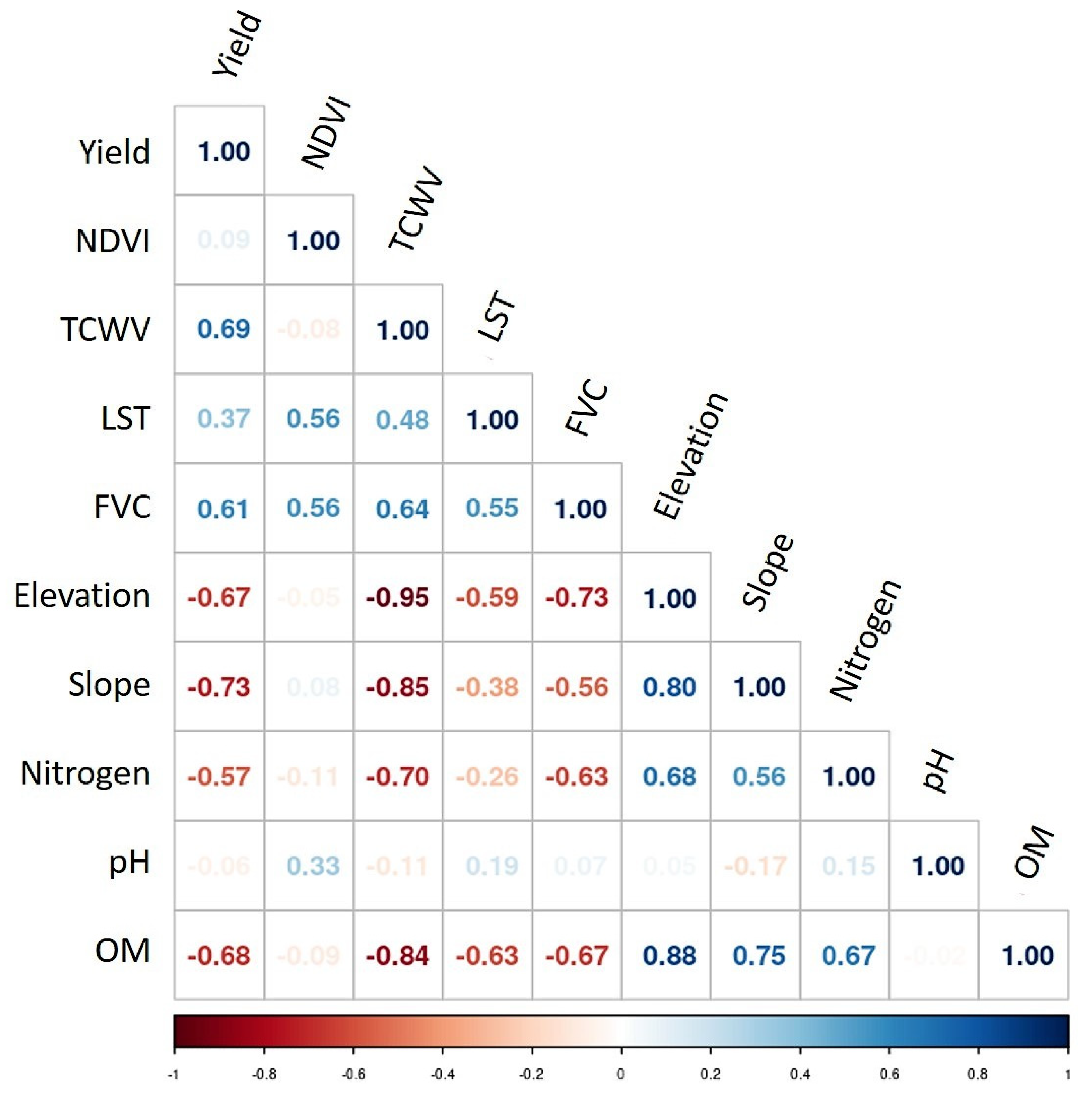
3.1. Descriptive Analysis

The descriptive analysis of reference data revealed a significant spatial variability, as evidenced by a substantial difference between the minimum yield of 1.15 t/ha in the Bhojpur district, eastern Nepal, and the maximum yield of 4.51 t/ha in the Chitawan district in the central south of the country. This disparity highlights the spatial variability in yield values across districts, as presented in

Table 3. Descriptive statistics of average wheat yield (t/ha) in Nepal for 2021.

Minimum	1st Qu.	Median	Mean	3rd Qu.	Maximum	Skewness
1.15	2.09	2.56	2.65	3.26	4.51	−0.009

. Furthermore, a normality test was conducted to assess the distribution of yield data. The results indicated that data followed a normal distribution, with a slight negative skewness of −0.009. This finding was further corroborated by the minimal difference between the mean and median values, indicating an overall symmetrical distribution.

Upon conducting the Mann–Kendall test, a statistical test used to analyze trends in data [88], a tau value of 0.04 was obtained. This value serves as a quantitative measure to assess the strength and direction of the observed trend in data. In this context, the tau value indicates the presence of a negligible trend. This test was performed in R Studio using the “kendall” package.

3.2. Selection of Variables and Model Calibration

To select the most informative variables on crop yield, Pearson correlation was conducted between wheat yield and explanatory variables retrieved from Sentinel-3 SLSTR data, soil maps, and DEM. The final results are illustrated in Figure 5. Among the examined features, slope, TCWV, OM, and elevation displayed the most significant correlation coefficients of −0.73, 0.69, −0.68, and −0.67, respectively. These results suggest that steeper slopes and elevated terrains tend to be associated with reduced yields, potentially due to the challenges in crop management and growth under such suboptimal conditions, which corroborates with Ferrara et al. [89] and Heil et al. [90] regarding topography impacts on crop yield variability under different climatic settings. In addition, a higher total column of water vapor indicates an increased crop yield. This further agrees with Hsiao et al. [91] regarding water vapor’s role in canopy growth, hence its productivity. Generally, a higher TCWV indicates reduced water stress responses in vegetation, such as increased photosynthetic rates and higher leaf area development, which considerably influences yields.

Although SOM plays a crucial role in crop growth, for wheat, its optimal range is typically between 2% and 4%. Interestingly, the analysis conducted in this study showed a wide variation in OM content, with mean values ranging between 1.1 and 6.2%. The correlation analysis did not support a typically positive relationship between OM and crop yields. This contradicts previous research findings [92,93] regarding the positive correlation between yield and SOM. However, a recent study by Vonk et al. [94] showed a poor association between yield data and SOM in some European territories, finding similar results under the Atlantic climate with an average of 75 kg/ha lower wheat yield on soils with increased SOM by 1%. Another study by Wood et al. [95] reported an opposite effect between yield and SOM. The latter study suggested that different SOM fractions are regulated by distinct mechanisms, which result in various associations with agricultural management outcomes intricately intertwined with environmental factors like topography, ultimately affecting crop productivity. These findings support the significance of the relationship between yield and SOM. Nevertheless, intensive research is needed to better understand the complex interactions in different scenarios.

Furthermore, a moderately high correlation coefficient of 0.61 was observed for FVC, indicating that a more significant fraction of vegetation cover signifies higher wheat yield. This agrees with the work of Cui et al. [96] regarding the positive correlation between FVC values and yield. As FVC represents the proportion of land surface covered by vegetation, a higher value suggests a greater density and extent of vegetation, a feature that can be influenced by soil fertility. Specifically, in the context of crops, fertile soils can sustain more abundant vegetation, thus resulting in increased FVC [97].

Total nitrogen content plays a fundamental role in canopy growth, including wheat, with an optimal range typically falling between 0.2% and 0.4% [98]. Our study observed a wide variation in nitrogen content across districts, ranging from 0.07% to 0.24%. Contrary to expectations, the analysis revealed a negative correlation of −0.57 between nitrogen content and yield, disagreeing with previous research work [99]. Notably, different fractions of total nitrogen are regulated by distinct processes, influencing crop productivity. For instance, a recent study by Sun et al. [100] has demonstrated that lower nitrogen content rates are beneficial for soil and leaf physiological factors, ultimately leading to enhanced crop yield. These findings highlight the significance of understanding the complex mechanisms involved in the relationship between total nitrogen content in soil and crop yield, further corroborating previous research work [101,102].

Different regions and altitudes in Nepal have distinct microclimates and temperature patterns [103]. In higher altitudes, cooler temperatures prevail, which have different implications for yield compared to slightly warmer lowland regions [104]. Therefore, the correlation between LST and wheat yield in Nepal depends on the study area’s specific elevation, canopy characteristics, and local climatic conditions. While wheat has an optimal temperature range for growth between 15 and 25 °C [105], the mean surface temperature exhibited a broader range in this study, spanning between −1.1 and 27.95 °C. It is essential to highlight that specific temporal patterns observed throughout the growing season can affect the relationship between LST and crop yield. In this context, a study conducted by Kern et al. [106], based on remote sensing data and climatic features, revealed that elevated temperatures during mid-season have a beneficial effect on wheat growth, hence its yield. In the present study, a weak correlation of 0.37 between crop yield and LST has been found, suggesting that although surface temperature may have an impact on wheat productivity, other factors exert a more substantial influence in determining the overall yield in Nepal. In essence, the temperature impact on crop yield depends on how well it aligns with the temperature requirements of the crop at different phenological stages, which can either be advantageous or detrimental, depending on its suitability for the specific crop growth stage. These observations are consistent with the findings of Musa et al. [107].

While NDVI is commonly used as an indicator of plant health and biomass, measuring vegetation greenness and density [108], our findings revealed a relatively weaker correlation between NDVI and crop yield. Consequently, we excluded NDVI, along with pH, for the same reason. This contradicts previous research on the potential of NDVI in crop yield estimation. For instance, Panek and Gozdowski [109] conducted a study focusing on NDVI during the March to May period and its correlation with crop yield. Their findings indicate that a 0.1 increase in NDVI leads to a remarkable improvement in crop yield, ranging from 1.1 to 2.6 t/ha based on MODIS data. This observation highlights the possibility of predicting regional-level crop yield 3 to 4 months before the harvest using solely NDVI. A more recent study by Roznik et al. [110] suggested that crop yield estimation modeling can be enhanced by including higher-resolution satellite data integrated with more precise cropland masks.

Although pH is a key factor for soil health and nutrient availability to crops [111], its relatively low significance in this study indicates that the mean pH levels, ranging from 5.6 to 7.7, did not exhibit a strong correlation with variations in wheat yield. Maintaining an optimal pH range of 6 to 7.5 is crucial for crop growth; however, other factors, such as agronomic practices and technological advancements, may have had a more substantial role in influencing the observed variations in wheat yield in this study.

These findings emphasize the complexity of interconnectedness between variables and wheat yield, suggesting that the impact of organic matter and total nitrogen content on crop productivity may vary depending on specific conditions and contexts [112,113]. As a result, key variables like slope, TCWV, OM, elevation, FVC, nitrogen content, and LST are used in the subsequent machine learning modeling phase to develop estimation models for wheat yield at the district level.

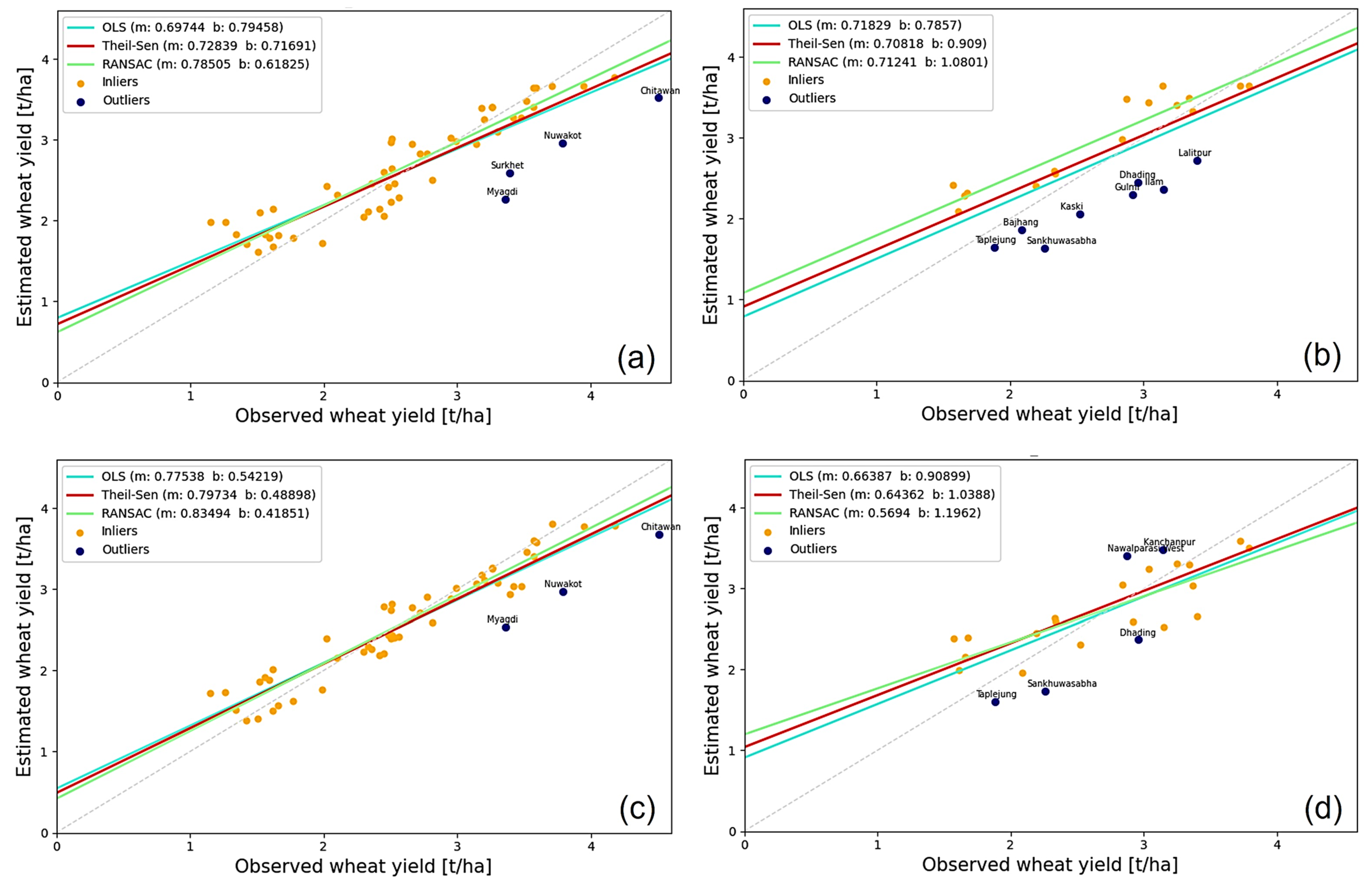
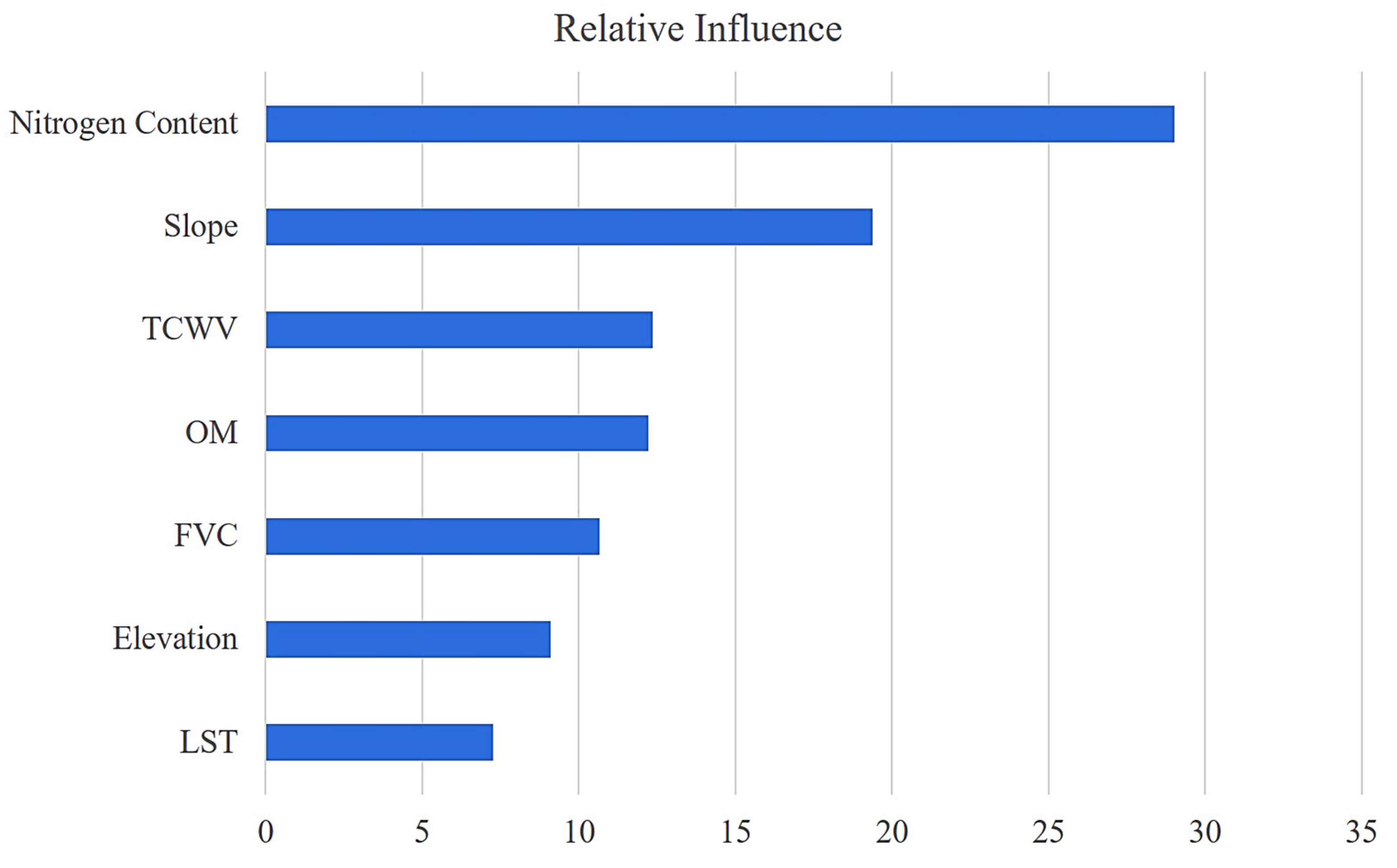
3.3. Accuracy Assessment and Influence of Features

A comparison of the GBM and XGBoost calibrated models revealed notable differences in their performance when predicting wheat yield using Sentinel-3 SLSTR data, soil information, and topographic features. The main results are illustrated in

Table 4. Performance of machine learning-based models in crop yield estimation using two statistical metrics in training and testing.

Model	Training		Testing
	R2	RMSE (t/ha)	R2	RMSE (t/ha)
GBM	0.79	0.38	0.56	0.47
XGBoost	0.89	0.30	0.61	0.42

.

Compared to the GBM model, the XGBoost model showed superior performance in predicting wheat yield, exhibiting an improvement of approximately 10% in accuracy for the training set and 5% for the testing set, as indicated by the increased R² and decreased RMSE values. This indicates that the XGBoost model effectively captures the underlying patterns and relationships between the variables, resulting in more accurate estimates for average wheat yield. These findings are in agreement with previous studies by Mariadass et al. [114], Kulpanich et al. [115], and Noorunnahar et al. [116], which have also highlighted the superior performance of the XGBoost algorithm compared to other machine learning models. A recent study by Huber et al. [117] explored the potential of XGBoost for soybean yield estimation in the United States, yielding an average R² of 0.79, which was outperformed by our XGBoost-based model. The same study suggested future research to focus on yield prediction on other crops based on XGBoost due to its superiority even to deep learning. Another research by Oikonomidis et al. [118] has evaluated machine learning for estimating crop yield across nine states in the United States using weather, soil, and agricultural management data. Several models were evaluated, including XGBoost, convolutional neural networks (CNN) combined with deep neural networks (DNN), CNN-XGBoost, CNN-recurrent neural networks (RNN), and CNN-long short-term memory (LSTM). Although the results indicated that the CNN-DNN model performed the best among the tested models, it is worth noting that the XGBoost model achieved the second-best performance while demanding less execution time compared to deep learning-based models. Their XGBoost model achieved an R² of 0.8, which our model surpassed with an R² of 0.89.

Figure 6 illustrates the linear correlation assessment of observed and estimated wheat yields. Notably, a closer alignment with reference data is exhibited by the XGBoost model, indicating a more robust association between the predicted and actual average wheat yield values. This further supports the superior statistical significance and predictive capabilities of XGBoost. Its improved performance can be attributed to its enhanced ability to handle complex relationships and interactions among the variables. As XGBoost effectively addresses the limitations of the GBM model, such as bias and variance, more accurate wheat yield estimates were expected. XGBoost incorporates enhancements that contribute to its robust performance, including regularization techniques, better processing of missing values, and the ability to handle non-linear relationships more effectively [85]. For example, Khan et al. [119] evaluated the performance of GBM and XGBoost, along with other machine learning algorithms, in maize yield prediction across France using meteorological data. The study demonstrated that XGBoost outperformed GBM, achieving an R² of 0.51 compared to an R² of 0.17 for GBM. Regardless, our established model yielded more accurate predictions compared to their findings. Furthermore, recent research conducted by Ahmed [120] to predict maize yield in the Saudi Arabia region based on weather data has further proven the potential of XGBoost in enhancing estimation accuracy compared to GBM. The study noted a decrease in RMSE value by 0.01 t/ha, indicating the improved performance of XGBoost in accurately predicting crop yield.

The analysis of wheat yield predictions reveals minimal heteroscedasticity, suggesting that only a few data points deviated from the overall trend. To explore this further, two robust regression methods, the Theil–Sen estimator [123,124] and the RANSAC algorithm [125,126], were applied to the data. Figure 6 illustrates the results obtained from these two methods alongside ordinary linear regression (OLS). While all three models (OLS, Theil–Sen estimator, and RANSAC) yielded comparable results, the latter two exhibited enhanced robustness. RANSAC successfully identified outliers that were excluded from the regression analysis. Both the RANSAC and Theil–Sen models performed well, leading to more reliable estimates. The number of identified outliers varied between the training and testing phases and between models based on different algorithms, such as GBM and XGBoost. During the testing phase, the RANSAC model identified a higher number of outliers for both XGBoost (5 outliers) and GBM (8 outliers) models, compared to the training phase (3 outliers for XGBoost and 4 outliers for GBM). This outcome is expected, as the testing phase involved new, unseen data that was not part of the training set. Notably, for XGBoost training, RANSAC highlighted three outliers: Chitawan, Myagdi, and Nuwakot. These districts are located in the central region of Nepal, in the transition physiographic zones between the Sivalik, low mountains, and high Himalayan regions. Previous research by Karki et al. [127] has characterized this area with a temperate climate masked by a dry winter and a warm to hot summer. Such climatic variability can contribute to unpredictability and fluctuations in agricultural productivity assessments. For testing, the outliers identified by RANSAC were predominantly situated in the middle mountain to the high Himalayan physiographic regions, which span a broad spectrum of climatic zones from tropical savannah to polar tundra. In this context, both least squares and Theil–Sen regression yielded comparable results, whereas the RANSAC model provided valuable insights into the specific behavior of data outliers. In addition, the RANSAC algorithm has effectively identified the inliers, predominantly located in the low-altitude flat areas characterized by expansive croplands. Although a few points in the middle region were identified as outliers, the districts in the Terai zone are primarily aligned with the overall trend, indicating a robust correlation between the actual and estimated wheat yield within these districts.

The behavior of points located in the Terai region motivated us to further inspect those districts separately, given their significance as the country’s primary agricultural land surface [128]. Remarkably, the districts within this region showed a close alignment in terms of correlation between observed and estimated wheat yield, with the XGBoost model demonstrating exceptional effectiveness in capturing the trends and patterns in the Terai districts. This led to significantly improved accuracy in wheat yield estimation in this region. These observations highlight the importance of considering regional variations and employing appropriate machine learning algorithms when analyzing agricultural data. Further, the varying number and geographic distribution of outliers elucidate the potential advantages of robust regression techniques in addressing datasets affected by heteroscedasticity and influential outliers in the context of crop yield assessment.

Integrating data on topography, soil quality, water content in the atmosphere, and vegetation density, leveraged by remote sensing techniques, is fundamental for accurately estimating crop yield. Based on the calibrated XGBoost, a demonstration of the most to least influential variables affecting yield estimation is presented in Figure 7. To assess the relative influence of used variables, we employed the feature importance approach, which measures the extent to which the model’s prediction error is affected when a feature is shuffled. As shuffling the feature values breaks the association between the variable and the outcome, the magnitude of the increase in prediction error reflects its importance, with a more significant increase indicating greater importance [129]. Among input variables, nitrogen content was identified as the most influential, significantly impacting wheat yield estimation. This finding is consistent with the observed distribution of average wheat yield per district, where lower nitrogen content tends to correlate with higher yields. Furthermore, variables like slope, total column water vapor, and organic matter have also revealed varying degrees of influence on crop yield, as highlighted in previous studies [130,131,132]. These features demonstrate great potential for application in agronomy-based studies and agricultural management systems. In contrast, land surface temperature (LST) was the least influential feature. A recent study indicated that the association between surface temperature and wheat yield is subject to complex interactions in both temporal and spatial dimensions [133]. These findings emphasize the importance of considering multiple influential variables, including nitrogen content, slope, total column water vapor, organic matter, FVC, and elevation. By incorporating these variables, researchers can improve the accuracy and reliability of yield estimates, enabling better-informed decision-making in agricultural management and food security initiatives at the national level.

Despite the superior performance of the XGBoost model in wheat yield estimation, there are still valuable opportunities for future research to enhance the capabilities of established models further. One potential avenue is integrating supplementary data associated with crop productivity, like nutrient management practices. Including additional variables that capture factors such as fertilization practices, pest and disease incidence, and irrigation management practices, can provide a more comprehensive insight into the complex dynamics that affect wheat yield within a spatio-temporal framework. Furthermore, acquiring extensive field data through detailed surveys, rather than relying solely on average values for districts, will significantly improve the accuracy of the established models. Collecting detailed data at the field level, including information on soil properties, crop phenology, and management practices, will enable a systematic analysis that effectively captures the spatial heterogeneity within agricultural landscapes. Higher-resolution data can also provide valuable insights into the factors governing crop yield variability at the country level, as demonstrated by Roznik et al. [110]. By incorporating multiple data sources and refining the model architecture, future studies can strive to predict and map crop yield distribution more accurately in similar environmental and climatic contexts.

4. Conclusions

This research aims to estimate wheat yield in Nepal using Sentinel-3 SLSTR, soil data, and topographic features. The study involved a comparative analysis of the performance of two machine learning models: gradient boosting machine (GBM) and extreme gradient boosting (XGBoost). The models were evaluated using the reference data on average yield per district in 2021. The findings indicated that the XGBoost model exhibited improved accuracy compared to GBM, with an increase of up to 10% in the coefficient of determination (R²) and a decrease in the root mean square error (RMSE).

The results highlight the potential of the established approach based on machine learning tools and geospatial data for crop yield estimation at the district level. The suggested approach successfully identified key relationships between various factors and wheat yield. Notably, the analysis revealed a positive correlation between average wheat yield and Sentinel-3 SLSTR-based features like fractional vegetation cover (FVC) and total column water vapor (TCWV), while altitude and slope negatively correlated with yield. Remarkably, soil factors such as organic matter and total nitrogen content exhibited a negative correlation with yield, which requires further investigation to grasp the underlying mechanisms and potential factors involved.

Considering the promising results obtained in terms of yield estimation, the suggested methodology demonstrates the potential for application in other study areas with comparable agricultural systems and climatic conditions. In the future, it can be enhanced by integrating real-time meteorological data with ground-based measurements. This would further facilitate monitoring agronomic practices and assessing their suitability at the farm level, given their significant impact on wheat yield.

Further research using alternative machine learning tools and data sources is recommended to enhance the model’s efficiency and thoroughly investigate the dynamics governing the relationships between the selected features and wheat yield. This would enable more accurate and timely monitoring, as well as early detection of yield anomalies in Nepal, aligning with Sustainable Development Goals (SDG2: Zero Hunger and SDG15: Life on Land).

References

1. Lobell, D.B.; Cassman, K.G.; Field, C.B. Crop yield gaps: Their importance, magnitudes, and causes. Annu. Rev. Environ. Resour. 2009, 34, 179–204. [Google Scholar] [CrossRef]
2. Carletto, C.; Jolliffe, D.; Banerjee, R. From tragedy to renaissance: Improving agricultural data for better policies. J. Dev. Stud. 2015, 51, 133–148. [Google Scholar] [CrossRef]
3. Dubey, S.; Dahiya, M.; Jain, S. Application of a distributed data center in logistics as cloud collaboration for handling disaster relief. In Proceedings of the IEEE 3rd International Conference on Internet of Things: Smart Innovation and Usages (IoT-SIU), Bhimtal, India, 23–24 February 2018; pp. 1–11. [Google Scholar] [CrossRef]
4. Mehdaoui, R.; Anane, M. Exploitation of the red-edge bands of Sentinel 2 to improve the estimation of durum wheat yield in Grombalia region (Northeastern Tunisia). Int. J. Remote Sens. 2020, 41, 8986–9008. [Google Scholar] [CrossRef]
5. Adhikari, S.P.; Ghimire, Y.N.; Timsina, K.P.; Subedi, S.; Kharel, M. Technical efficiency of wheat growing farmers of Nepal. J. Agric. Nat. Resour. 2021, 4, 246–254. [Google Scholar] [CrossRef]
6. Bognár, P.; Ferencz, C.; Pásztor, S.; Molnár, G.; Timár, G.; Hamar, D.; Lichtenberger, J.; Székely, B.; Steinbach, P.; Ferencz, O.E. Yield forecasting for wheat and corn in Hungary by satellite remote sensing. Int. J. Remote Sens. 2011, 32, 4759–4767. [Google Scholar] [CrossRef]
7. Zhu, B.; Chen, S.; Cao, Y.; Xu, Z.; Yu, Y.; Han, C. A Regional Maize Yield Hierarchical Linear Model Combining Landsat 8 Vegetative Indices and Meteorological Data: Case Study in Jilin Province. Remote Sens. 2021, 13, 356. [Google Scholar] [CrossRef]
8. Johnson, D.M.; Rosales, A.; Mueller, R.; Reynolds, C.; Frantz, R.; Anyamba, A.; Pak, E.; Tucker, C. USA Crop Yield Estimation with MODIS NDVI: Are Remotely Sensed Models Better than Simple Trend Analyses? Remote Sens. 2021, 13, 4227. [Google Scholar] [CrossRef]
9. Khaki, S.; Wang, L. Crop Yield Prediction Using Deep Neural Networks. Front. Plant Sci. 2019, 10, 621. [Google Scholar] [CrossRef]
10. Muruganantham, P.; Wibowo, S.; Grandhi, S.; Samrat, N.H.; Islam, N. A Systematic Literature Review on Crop Yield Prediction with Deep Learning and Remote Sensing. Remote Sens. 2022, 14, 1990. [Google Scholar] [CrossRef]
11. Abdul-Jabbar, T.S.; Ziboon, A.T.; Albayati, M.M. Crop yield estimation using different remote sensing data: Literature review. IOP Conf. Ser. Earth Environ. Sci. 2023, 1129, 012004. [Google Scholar] [CrossRef]
12. Ang, Y.; Shafri, H.Z.M.; Lee, Y.P.; Bakar, S.A.; Abidin, H.; Junaidi, M.U.U.M.; Samad, M.N.A. Oil Palm Yield Prediction Across Blocks Using Multi-Source Data and Machine Learning. Earth Sci. Inform. 2022, 15, 2349–2367. [Google Scholar] [CrossRef]
13. Yli-Heikkilä, M.; Wittke, S.; Luotamo, M.; Puttonen, E.; Sulkava, M.; Pellikka, P.; Heiskanen, J.; Klami, A. Scalable Crop Yield Prediction with Sentinel-2 Time Series and Temporal Convolutional Network. Remote Sens. 2022, 14, 4193. [Google Scholar] [CrossRef]
14. Saad El Imanni, H.; El Harti, A.; El Iysaouy, L. Wheat Yield Estimation Using Remote Sensing Indices Derived from Sentinel-2 Time Series and Google Earth Engine in a Highly Fragmented and Heterogeneous Agricultural Region. Agronomy 2022, 12, 2853. [Google Scholar] [CrossRef]
15. Bognár, P.; Kern, A.; Pásztor, S.; Lichtenberger, J.; Koronczay, D.; Ferencz, C.S. Yield estimation and forecasting for winter wheat in Hungary using time series of MODIS data. Int. J. Remote Sens. 2017, 38, 3394–3414. [Google Scholar] [CrossRef]
16. Hosseini, M.; Becker-Reshef, I.; Sahajpal, R.; Fontana, L.; Lafluf, P.; Leale, G.; Puricelli, E.; Varela, M.; Justice, C.J. Crop yield prediction using integration of polarimetric synthetic aperture radar and optical data. In Proceedings of the IEEE International Geoscience and Remote Sensing Symposium (IGARSS 2020), Waikoloa, HI, USA, 26 September–2 October 2020; pp. 17–20. [Google Scholar] [CrossRef]
17. Ouattara, B.; Forkuor, G.; Zoungrana, B.J.; Dimobe, K.; Danumah, J.; Saley, B.; Tondoh, J.E. Crops monitoring and yield estimation using sentinel products in semi-arid smallholder irrigation schemes. Int. J. Remote Sens. 2020, 41, 6527–6549. [Google Scholar] [CrossRef]
18. Roznik, M.; Mishra, A.K.; Boyd, M.S. Using a Machine Learning Approach and Big Data to Augment WASDE Forecasts: Empirical Evidence from US Corn Yield. J. Forecast. 2023, 42, 1370–1384. [Google Scholar] [CrossRef]
19. Bognár, P.; Kern, A.; Pásztor, S.; Steinbach, P.; Lichtenberger, J. Testing the Robust Yield Estimation Method for Winter Wheat, Corn, Rapeseed, and Sunflower with Different Vegetation Indices and Meteorological Data. Remote Sens. 2022, 14, 2860. [Google Scholar] [CrossRef]
20. Srivastava, A.K.; Safaei, N.; Khaki, S.; Lopez, G.; Zeng, W.; Ewert, F.; Gaiser, T.; Rahimi, J. Winter wheat yield prediction using convolutional neural networks from environmental and phenological data. Sci. Rep. 2022, 12, 3215. [Google Scholar] [CrossRef]
21. Cheng, E.; Zhang, B.; Peng, D.; Zhong, L.; Yu, L.; Liu, Y.; Xiao, C.; Li, C.; Li, X.; Chen, Y.; et al. Wheat yield estimation using remote sensing data based on machine learning approaches. Front. Plant Sci. 2022, 13, 1090970. [Google Scholar] [CrossRef]
22. Ramos, A.P.; Osco, L.P.; Furuya, D.E.; Gonçalves, W.N.; Santana, D.C.; Teodoro, L.P.; Junior, C.A.; Capristo-Silva, G.F.; Li, J.; Baio, F.H.; et al. A random forest ranking approach to predict yield in maize with uav-based vegetation spectral indices. Comput. Electron. Agric. 2020, 178, 105791. [Google Scholar] [CrossRef]
23. Joshi, A.; Pradhan, B.; Gite, S.; Chakraborty, S. Remote-Sensing Data and Deep-Learning Techniques in Crop Mapping and Yield Prediction: A Systematic Review. Remote Sens. 2023, 15, 2014. [Google Scholar] [CrossRef]
24. Arumugam, P.; Chemura, A.; Schauberger, B.; Gornott, C. Remote Sensing Based Yield Estimation of Rice (Oryza sativa L.) Using Gradient Boosted Regression in India. Remote Sens. 2021, 13, 2379. [Google Scholar] [CrossRef]
25. Pazhanivelan, S.; Geethalakshmi, V.; Tamilmounika, R.; Sudarmanian, N.S.; Kaliaperumal, R.; Ramalingam, K.; Sivamurugan, A.P.; Mrunalini, K.; Yadav, M.K.; Quicho, E.D. Spatial Rice Yield Estimation Using Multiple Linear Regression Analysis, Semi-Physical Approach and Assimilating SAR Satellite Derived Products with DSSAT Crop Simulation Model. Agronomy 2022, 12, 2008. [Google Scholar] [CrossRef]
26. Ilyas, Q.M.; Ahmad, M.; Mehmood, A. Automated Estimation of Crop Yield Using Artificial Intelligence and Remote Sensing Technologies. Bioengineering 2023, 10, 125. [Google Scholar] [CrossRef]
27. Al-Adhaileh, M.H.; Aldhyani, T.H.H. Artificial intelligence framework for modeling and predicting crop yield to enhance food security in Saudi Arabia. PeerJ. Comput. Sci. 2022, 8, e1104. [Google Scholar] [CrossRef] [PubMed]
28. Wolanin, A.; Mateo-García, G.; Camps-Valls, G.; Gómez-Chova, L.; Meroni, M.; Duveiller, G.; Liangzhi, Y.; Guanter, L. Estimating and understanding crop yields with explainable deep learning in the Indian Wheat Belt. Environ. Res. Lett. 2020, 15, 024019. [Google Scholar] [CrossRef]
29. Ferencz, C.; Bognár, P.; Lichtenberger, J.; Hamar, D.; Tarcsai, G.; Timár, G.; Molnár, G.; Pásztor, S.; Steinbach, P.; Székely, B.; et al. Crop yield estimation by satellite remote sensing. Int. J. Remote Sens. 2004, 25, 4113–4149. [Google Scholar] [CrossRef]
30. Franch, B.; Bautista, A.S.; Fita, D.; Rubio, C.; Tarrazó-Serrano, D.; Sánchez, A.; Skakun, S.; Vermote, E.; Becker-Reshef, I.; Uris, A. Within-Field Rice Yield Estimation Based on Sentinel-2 Satellite Data. Remote Sens. 2021, 13, 4095. [Google Scholar] [CrossRef]
31. Adebayo, A.D.; Sahbeni, G.; Donike, S. Integration of Sentinel-1 SAR and Sentinel-2 MSI time series DATA for crop yield prediction over agricultural areas in Kenya. In Proceedings of the AGIT2021 Conference, Salzburg, Austria, 5–9 July 2021. [Google Scholar] [CrossRef]
32. Bojanowski, J.S.; Sikora, S.; Musiał, J.P.; Woźniak, E.; Dąbrowska-Zielińska, K.; Slesiński, P.; Milewski, T.; Łączyński, A. Integration of Sentinel-3 and MODIS Vegetation Indices with ERA-5 Agro-Meteorological Indicators for Operational Crop Yield Forecasting. Remote Sens. 2022, 14, 1238. [Google Scholar] [CrossRef]
33. Chhetri, R.; Pandey, V.P.; Talchabhadel, R.; Thapa, B.R. How do CMIP6 models project changes in precipitation extremes over seasons and locations across the mid hills of Nepal? Theor. Appl. Climatol. 2021, 145, 1127–1144. [Google Scholar] [CrossRef]
34. Sharma, S.; Khadka, N.; Hamal, K.; Baniya, B.; Luintel, N.; Joshi, B.B. Spatial and temporal analysis of precipitation and its extremities in seven provinces of Nepal (2001–2016). Appl. Ecol. Environ. Sci. 2020, 8, 64–73. [Google Scholar] [CrossRef]
35. Upreti, B.N. An overview of the stratigraphy and tectonics of the Nepal Himalaya. J. Asian Earth Sci. 1999, 17, 577–606. [Google Scholar] [CrossRef]
36. Bhattarai, T.N. Flood Events in Gangapur Village, Banke District: An Example of Climate Change-Induced Disaster in Nepal. J. Inst. Sci. Technol. 2014, 19, 79–85. [Google Scholar] [CrossRef]
37. Peel, M.C.; Finlayson, B.L.; McMahon, T.A. Updated world map of the Köppen-Geiger climate classification. Hydrol. Earth Syst. Sci. 2007, 5, 1633–1644. [Google Scholar] [CrossRef]
38. Dai, W.; Subedi, R.; Jin, K.; Hao, L. Spatiotemporal variation of potential evapotranspiration and meteorological drought based on multi-source data in Nepal. Nat. Hazards Res. 2023, 3, 271–279. [Google Scholar] [CrossRef]
39. Karki, R.; Ul Hasson, S.; Gerlitz, L.; Talchabhadel, R.; Schickhoff, U.; Scholten, T.; Böhner, J. Rising mean and extreme near-surface air temperature across Nepal. Int. J. Climatol. 2020, 40, 2445–2463. [Google Scholar] [CrossRef]
40. Ba, R.; Zech, W. Soils of the high mountain region of Eastern Nepal: Classification, distribution, and soil forming processes. Catena 1994, 22, 85–103. [Google Scholar] [CrossRef]
41. Merz, J. Water Balances, Floods and Sediment Transport in the Hindu Kush-Himalayan Region; Geographical Bernensia. G72; Department of Geography, University of Bern, Bern and International Centre for Integrated Mountain Development: Kathmandu, Nepal, 2004. [Google Scholar] [CrossRef]
42. Paudel, B.; Zhang, Y.L.; Li, S.C.; Liu, L.S.; Wu, X.; Khanal, N.R. Review of studies on land use and land cover change in Nepal. J. Mt. Sci. 2016, 13, 643–660. [Google Scholar] [CrossRef]
43. Gairhe, S.; Shrestha, H.K.; Timsina, K. Dynamics of major cereals productivity in Nepal. J. Nepal Agric. Res. Counc. 2018, 4, 60–71. [Google Scholar] [CrossRef]
44. The World Bank. Population, Total—Nepal. 2021. Available online: https://data.worldbank.org/indicator/SP.POP.TOTL?locations=NP (accessed on 30 March 2023).
45. National Planning Commission. Sustainable Development Goals (Kathmandu, Nepal: Government of Nepal, National Planning Commission. 2017. Available online: https://www.npc.gov.np/images/category/SDGs_Report_Final.pdf (accessed on 30 March 2023).
46. Joshi, K.D.; Conroy, C.; Witcombe, J.R. Agriculture, seed, and innovation in Nepal: Industry and policy issues for the future. Gates Open Res. 2019, 3, 232. [Google Scholar] [CrossRef]
47. Ministry of Agriculture and Livestock Development, Government of Nepal. Statistical Information on Nepalese Agriculture—2020/21 (Report No. 2077/78). 2021. Available online: https://nepalindata.com/resource/STATISTICAL-INFORMATION-ON-NEPALESE-AGRICULTURE-2077-78--2020-21/ (accessed on 30 March 2023).
48. ESA. User Guides. Available online: https://sentinels.copernicus.eu/web/sentinel/user-guides.2022 (accessed on 5 June 2023).
49. Coppo, P.; Ricciarelli, B.; Brandani, F.; Delderfield, J.; Ferlet, M.; Mutlow, C.; Munro, G.; Nightingale, T.; Smith, D.; Bianchi, S.; et al. SLSTR: A high accuracy dual scan temperature radiometer for sea and land surface monitoring from space. J. Mod. Opt. 2010, 57, 1815–1830. [Google Scholar] [CrossRef]
50. Musyimi, P.K.; Sahbeni, G.; Timár, G.; Weidinger, T.; Székely, B. Analysis of Short-Term Drought Episodes Using Sentinel-3 SLSTR Data under a Semi-Arid Climate in Lower Eastern Kenya. Remote Sens. 2023, 15, 3041. [Google Scholar] [CrossRef]
51. Hu, X.; Ren, H.; Tansey, K.; Zheng, Y.; Ghent, D.; Liu, X.; Yan, L. Agricultural drought monitoring using European Space Agency Sentinel 3A land surface temperature and normalized difference vegetation index imageries. Agric. For. Meteorol. 2019, 279, 107707. [Google Scholar] [CrossRef]
52. Musyimi, P.K.; Sahbeni, G.; Timár, G.; Weidinger, T.; Székely, B. Actual Evapotranspiration Estimation Using Sentinel-1 SAR and Sentinel-3 SLSTR Data Combined with a Gradient Boosting Machine Model in Busia County, Western Kenya. Atmosphere 2022, 13, 1927. [Google Scholar] [CrossRef]
53. Xu, W.; Wooster, M.J. Sentinel-3 SLSTR active fire (AF) detection and FRP daytime product—Algorithm description and global intercomparison to MODIS, VIIRS and Landsat AF data. Sci. Remote Sens. 2023, 7, 100087. [Google Scholar] [CrossRef]
54. Ojha, N.; Merlin, O.; Suere, C.; Escorihuela, M.J. Extending the Spatio-Temporal Applicability of DISPATCH Soil Moisture Downscaling Algorithm: A Study Case Using SMAP, MODIS and Sentinel-3 Data. Front. Environ. Sci. 2021, 9, 555216. [Google Scholar] [CrossRef]
55. IPAD. Country Summary—Nepal Production. 2023. Available online: https://ipad.fas.usda.gov/countrysummary/default.aspx?id=NP (accessed on 15 April 2023).
56. Sahbeni, G.; Székely, B.; Sahajpal, R. Characterization of different crop types using biophysical indicators derived from Sentinel-2 MSI multi-temporal data in Sudurpashchim Province, Western Nepal. In Proceedings of the EGU General Assembly 2023, Vienna, Austria, 24–28 April 2023. EGU23-3884. [Google Scholar] [CrossRef]
57. NASA Shuttle Radar Topography Mission (SRTM). Shuttle Radar Topography Mission (SRTM) Global. Distributed by OpenTopography 2013. Available online: https://www.fdsn.org/networks/detail/GH/ (accessed on 5 June 2023).
58. Open Topography. Three New Global Topographic Datasets Available (SRTM Ellipsoidal, ALOS World 3D, GMRT). 2017. Available online: https://opentopography.org/news/three-new-global-topographic-datasets-available-srtm-ellipsoidal-alos-world-3d-gmrt (accessed on 31 March 2023).
59. Arino, O.; Gross, D.; Ranera, F.; Bourg, L.; Leroy, M.; Bicheron, P.; Latham, J.; Di Gregorio, A.; Brockmann, C.; Witt, R.; et al. GlobCover: ESA Service for Global Land Cover from MERIS. In Proceedings of the IEEE International Geoscience and Remote Sensing Symposium, Barcelona, Spain, 23–28 July 2007; pp. 2412–2415, JRC49403. [Google Scholar] [CrossRef]
60. ESA. Copernicus Sentinel-3 SLSTR Land User Handbook. 2023. Available online: https://sentinel.esa.int/documents/247904/4598082/Sentinel-3-SLSTR-Land-Handbook.pdf (accessed on 20 February 2023).
61. Kganyago, M.; Mhangara, P.; Adjorlolo, C. Estimating Crop Biophysical Parameters Using Machine Learning Algorithms and Sentinel-2 Imagery. Remote Sens. 2021, 13, 4314. [Google Scholar] [CrossRef]
62. Fan, J.; Ma, X.; Wu, L.; Zhang, F.; Yu, X.; Zeng, W. Light Gradient Boosting Machine: An efficient soft computing model for estimating daily reference evapotranspiration with local and external meteorological data. Agric. Water Manag. 2019, 225, 105758. [Google Scholar] [CrossRef]
63. Wang, L.; Hu, P.; Zheng, H.; Liu, Y.; Cao, X.; Hellwich, O.; Liu, T.; Luo, G.; Bao, A.; Chen, X. Integrative modeling of heterogeneous soil salinity using sparse ground samples and remote sensing images. Geoderma 2023, 430, 116321. [Google Scholar] [CrossRef]
64. He, Z.; Lin, D.; Lau, T.; Wu, M. Gradient Boosting Machine: A Survey. arXiv 2019, arXiv:1908.06951. [Google Scholar] [CrossRef]
65. Aworka, R.; Cedric, L.S.; Adoni, W.Y.; Zoueu, J.T.; Mutombo, F.K.; Kimpolo, C.L.; Nahhal, T.; Krichen, M. Agricultural Decision System based on Advanced Machine Learning Models for Yield Prediction: Case of East African Countries. Smart Agric. Technol. 2022, 2, 100048. [Google Scholar] [CrossRef]
66. Landry, M. Machine Learning with R and H2O; H2O. ai: Mountain View, CA, USA, 2016; Available online: http://h2o-release.s3.amazonaws.com/h2o/master/5118/docs-website/h2o-docs/booklets/RBooklet.pdf (accessed on 16 April 2023).
67. Lu, H.; Karimireddy, S.P.; Ponomareva, N.; Mirrokni, V.S. Accelerating Gradient Boosting Machines. In Proceedings of the 23rd International Conference on Artificial Intelligence and Statistics (AISTATS 2020), Palermo, Italy, 26–28 August 2020; Volume 108. Available online: http://proceedings.mlr.press/v108/lu20a/lu20a.pdf (accessed on 19 April 2023).
68. Candido, C.G.; Blanco, A.C.; Medina, J.M.; Gubatanga, E.; Santos, A.; Ana, R.C.; Reyes, R.B. Improving the consistency of multi-temporal land cover mapping of Laguna Lake watershed using light gradient boosting machine (LightGBM) approach, change detection analysis, and Markov chain. Remote Sens. Appl. Soc. Environ. 2021, 23, 100565. [Google Scholar] [CrossRef]
69. Khoi, D.N.; Quan, N.T.; Linh, D.Q.; Nhi, P.T.T.; Thuy, N.T.D. Using Machine Learning Models for Predicting the Water Quality Index in the La Buong River, Vietnam. Water 2022, 14, 1552. [Google Scholar] [CrossRef]
70. Friedman, J. Greedy boosting approximation: A gradient boosting machine. Ann. Stat. 2001, 29, 1189–1232. [Google Scholar] [CrossRef]
71. Sarijaloo, F.B.; Porta, M.; Taslimi, B.; Pardalos, P.M. Yield performance estimation of corn hybrids using machine learning algorithms. Artif. Intell. Agric. 2021, 5, 82–89. [Google Scholar] [CrossRef]
72. Park, J.; Lee, Y.; Lee, J. Assessment of Machine Learning Algorithms for Land Cover Classification Using Remotely Sensed Data. Sens. Mater. 2021, 33, 3885–3902. [Google Scholar] [CrossRef]
73. Tarwidi, D.; Pudjaprasetya, S.R.; Adytia, D.; Apri, M. An optimized XGBoost-based machine learning method for predicting wave run-up on a sloping beach. MethodsX 2023, 10, 102119. [Google Scholar] [CrossRef]
74. Zopluoglu, C. How Does Extreme Gradient Boosting (XGBoost) Work? 2019. Available online: https://github.com/czopluoglu/website/tree/master/docs/posts/extreme-gradient-boosting/ (accessed on 11 May 2023).
75. Nalluri, M.; Pentela, M.; Eluri, N.R. A Scalable Tree Boosting System: XG Boost. Int. J. Res. Stud. Sci. Eng. Technol. 2020, 7, 36–51. [Google Scholar]
76. Zhang, P.; Jia, Y.; Shang, Y. Research and application of XGBoost in imbalanced data. Int. J. Distrib. Sens. Netw. 2022, 18, 15501329221106935. [Google Scholar] [CrossRef]
77. Guo, R.; Zhao, Z.; Wang, T.; Liu, G.; Zhao, J.; Gao, D. Degradation State Recognition of Piston Pump Based on ICEEMDAN and XGBoost. Appl. Sci. 2020, 10, 6593. [Google Scholar] [CrossRef]
78. Ali, Y.A.; Awwad, E.M.; Al-Razgan, M.; Maarouf, A. Hyperparameter Search for Machine Learning Algorithms for Optimizing the Computational Complexity. Processes 2023, 11, 349. [Google Scholar] [CrossRef]
79. Liashchynskyi, P.; Liashchynskyi, P. Grid search, random search, genetic algorithm: A big comparison for NAS. arXiv 2019, arXiv:1912.06059. [Google Scholar] [CrossRef]
80. Bergstra, J.; Bengio, Y. Random search for hyper-parameter optimization. J. Mach. Learn. Res. 2012, 13, 281–305. [Google Scholar]
81. Larochelle, H.; Erhan, D.; Courville, A.; Bergstra, J.; Bengio, Y. An empirical evaluation of deep architectures on problem with many factors of variation. In Proceedings of the Twenty-Fourth International Conference on Machine Learning (ICML’07), Corvallis, OR, USA, 20–24 June 2007; pp. 473–480. [Google Scholar] [CrossRef]
82. Natekin, A.; Knoll, A. Gradient boosting machines, a tutorial. Front. Neurorobot. 2013, 7, 21. [Google Scholar] [CrossRef] [PubMed]
83. Boehmke, B.; Greenwell, B.M. Chapter 12. In Gradient Boosting, Hands-On Machine Learning with R, 1st ed.; Chapman and Hall, CRC: London, UK, 2019. [Google Scholar]
84. Arif Ali, Z.; Abduljabbar, Z.H.; Taher, H.A.; Bibo Sallow, A.; Almufti, S.M. Exploring the Power of eXtreme Gradient Boosting Algorithm in Machine Learning: A Review. Acad. J. Nawroz Univ. 2023, 12, 320–334. [Google Scholar] [CrossRef]
85. Chen, T.; Guestrin, C. XGBoost: A Scalable Tree Boosting System. In Proceedings of the 22nd ACM SIGKDD International Conference on Knowledge Discovery and Data Mining, San Francisco, CA, USA, 13–17 August 2016; pp. 785–794. [Google Scholar] [CrossRef]
86. Bentéjac, C.; Csörgő, A.; Martínez-Muñoz, G. A comparative analysis of gradient boosting algorithms. Artif. Intell. Rev. 2021, 54, 1937–1967. [Google Scholar] [CrossRef]
87. Pham, H.T.; Awange, J.; Kuhn, M.; Nguyen, B.V.; Bui, L.K. Enhancing Crop Yield Prediction Utilizing Machine Learning on Satellite-Based Vegetation Health Indices. Sensors 2022, 22, 719. [Google Scholar] [CrossRef]
88. Ali, R.; Kuriqi, A.; Abubaker, S.; Kisi, O. Long-Term Trends and Seasonality Detection of the Observed Flow in Yangtze River Using Mann-Kendall and Sen’s Innovative Trend Method. Water 2019, 11, 1855. [Google Scholar] [CrossRef]
89. Ferrara, R.M.; Trevisiol, P.; Acutis, M.; Rana, G.; Richter, G.M.; Baggaley, N. Topographic impacts on wheat yields under climate change: Two contrasted case studies in Europe. Theor. Appl. Climatol. 2010, 99, 53–65. [Google Scholar] [CrossRef]
90. Heil, K.; Heinemann, P.; Schmidhalter, U. Modeling the Effects of Soil Variability, Topography, and Management on the Yield of Barley. Front. Environ. Sci. 2018, 6, 146. [Google Scholar] [CrossRef]
91. Hsiao, J.; Swann, A.L.; Kim, S. Maize yield under a changing climate: The hidden role of vapor pressure deficit. Agric. For. Meteorol. 2018, 297, 107692. [Google Scholar] [CrossRef]
92. King, A.E.; Ali, G.A.; Gillespie, A.W.; Wagner-Riddle, C. Soil Organic Matter as Catalyst of Crop Resource Capture. Front. Environ. Sci. 2020, 8, 50. [Google Scholar] [CrossRef]
93. Oldfield, E.E.; Bradford, M.A.; Augarten, A.J.; Cooley, E.T.; Radatz, A.M.; Radatz, T.; Ruark, M.D. Positive associations of soil organic matter and crop yields across a regional network of working farms. Soil Sci. Soc. Am. J. 2021, 86, 384–397. [Google Scholar] [CrossRef]
94. Vonk, W.J.; van Ittersum, M.K.; Reidsma, P.; Zavattaro, L.; Bechini, L.; Guzmán, G.; Pronk, A.; Spiegel, H.; Steinmann, H.H.; Ruysschaert, G.; et al. European survey shows poor association between soil organic matter and crop yields. Nutr. Cycl. Agroecosyst. 2020, 118, 325–334. [Google Scholar] [CrossRef]
95. Wood, S.A.; Sokol, N.; Bell, C.W.; Bradford, M.A.; Naeem, S.; Wallenstein, M.D.; Palm, C.A. Opposing effects of different soil organic matter fractions on crop yields. Ecol. Appl. A Publ. Ecol. Soc. Am. 2016, 26, 2072–2085. [Google Scholar] [CrossRef]
96. Cui, Y.; Liu, S.; Li, X.; Geng, H.; Xie, Y.; He, Y. Estimating Maize Yield in the Black Soil Region of Northeast China Using Land Surface Data Assimilation: Integrating a Crop Model and Remote Sensing. Front. Plant Sci. 2022, 13, 915109. [Google Scholar] [CrossRef]
97. Martin, A.J. Parry and others, Raising yield potential of wheat. II. Increasing photosynthetic capacity and efficiency. J. Exp. Bot. 2011, 62, 453–467. [Google Scholar] [CrossRef]
98. Anas, M.; Liao, F.; Verma, K.K.; Sarwar, M.A.; Mahmood, A.; Chen, Z.L.; Li, Q.; Zeng, X.P.; Liu, Y.; Li, Y.R. Fate of nitrogen in agriculture and environment: Agronomic, eco-physiological and molecular approaches to improve nitrogen use efficiency. Biol. Res. 2020, 53, 47. [Google Scholar] [CrossRef]
99. Boulelouah, N.; Berbache, M.R.; Bedjaoui, H.; Selama, N.; Rebouh, N.Y. Influence of Nitrogen Fertilizer Rate on Yield, Grain Quality and Nitrogen Use Efficiency of Durum Wheat (Triticum durum Desf) under Algerian Semiarid Conditions. Agriculture 2022, 12, 1937. [Google Scholar] [CrossRef]
100. Sun, J.; Li, W.; Li, C.; Chang, W.; Zhang, S.; Zeng, Y.; Zeng, C.; Peng, M. Effect of Different Rates of Nitrogen Fertilization on Crop Yield, Soil Properties and Leaf Physiological Attributes in Banana Under Subtropical Regions of China. Front. Plant Sci. 2020, 11, 613760. [Google Scholar] [CrossRef]
101. Belete, F.; Dechassa, N.; Molla, A.; Tana, T. Effect of nitrogen fertilizer rates on grain yield and nitrogen uptake and use efficiency of bread wheat (Triticum aestivum L.) varieties on the Vertisols of central highlands of Ethiopia. Agric. Food Secur. 2018, 7, 78. [Google Scholar] [CrossRef]
102. Ma, G.; Liu, W.; Li, S.; Zhang, P.; Wang, C.; Lu, H.; Wang, L.; Xie, Y.; Ma, D.; Kang, G. Determining the Optimal N Input to Improve Grain Yield and Quality in Winter Wheat with Reduced Apparent N Loss in the North China Plain. Front. Plant Sci. 2019, 10, 181. [Google Scholar] [CrossRef] [PubMed]
103. Luitel, D.R.; Jha, P.K.; Siwakoti, M.; Shrestha, M.L.; Munniappan, R. Climatic Trends in Different Bioclimatic Zones in the Chitwan Annapurna Landscape, Nepal. Climate 2020, 8, 136. [Google Scholar] [CrossRef]
104. Dawadi, B.; Shrestha, A.; Acharya, R.; Dhital, Y.P.; Devkota, R. Impact of climate change on agricultural production: A case of Rasuwa District, Nepal. Reg. Sustain. 2022, 3, 122–132. [Google Scholar] [CrossRef]
105. Acevedo, E.; Silva, P.; Silva, H. Wheat growth and physiology. In FAO Corporate Repository; FAO: Rome, Italy, 2009; pp. 1–24. [Google Scholar]
106. Kern, A.; Barcza, Z.; Marjanović, H.; Árendás, T.; Fodor, N.; Bónis, P.; Bognár, P.; Lichtenberger, J. Statistical modelling of crop yield in Central Europe using climate data and remote sensing vegetation indices. Agric. For. Meteorol. 2018, 260, 300–320. [Google Scholar] [CrossRef]
107. Musa, A.I.; Tsubo, M.; Ali-Babiker, I.E.A.; Iizumi, T.; Kurosaki, Y.; Ibaraki, Y.; El-Hag, F.M.; Tahir, I.S.; Tsujimoto, H. Relationship of irrigated wheat yield with temperature in hot environments of Sudan. Theor. Appl. Climatol. 2021, 145, 1113–1125. [Google Scholar] [CrossRef]
108. Cabrera-Bosquet, L.; Molero, G.; Stellacci, A.; Bort, J.; Nogués, S.; Araus, J. NDVI as a potential tool for predicting biomass, plant nitrogen content and growth in wheat genotypes subjected to different water and nitrogen conditions. Cereal Res. Commun. 2011, 39, 147–159. [Google Scholar] [CrossRef]
109. Panek, E.; Gozdowski, D. Analysis of relationship between cereal yield and NDVI for selected regions of Central Europe based on MODIS satellite data. Remote Sens. Appl. Soc. Environ. 2020, 17, 100286. [Google Scholar] [CrossRef]
110. Roznik, M.; Boyd, M.; Porth, L. Improving crop yield estimation by applying higher resolution satellite NDVI imagery and high-resolution cropland masks. Remote Sens. Appl. Soc. Environ. 2022, 25, 100693. [Google Scholar] [CrossRef]
111. Barrow, N.J.; Hartemink, A.E. The effects of pH on nutrient availability depend on both soils and plants. Plant Soil 2023, 487, 21–37. [Google Scholar] [CrossRef]
112. Chen, J.; Manevski, K.; Lærke, P.E.; Jørgensen, U. Biomass yield, yield stability and soil carbon and nitrogen content under cropping systems destined for biorefineries. Soil Tillage Res. 2022, 221, 105397. [Google Scholar] [CrossRef]
113. McLachlan, B.A.; van Kooten, G.C.; Zheng, Z. Country-level climate-crop yield relationships and the impacts of climate change on food security. SN Appl. Sci. 2020, 2, 1650. [Google Scholar] [CrossRef]
114. Mariadass, D.A.L.; Moung, E.G.; Sufian, M.M.; Farzamnia, A. EXtreme gradient boosting (XGBoost) regressor and shapley additive explanation for crop yield prediction in agriculture. In Proceedings of the 12th International Conference on Computer and Knowledge Engineering (ICCKE), Mashhad, Iran, 17–18 November 2022; pp. 219–224. [Google Scholar] [CrossRef]
115. Kulpanich, N.; Worachairungreung, M.; Thanakunwutthirot, K.; Chaiboonrueang, P. The Application of Unmanned Aerial Vehicles (UAVs) and Extreme Gradient Boosting (XGBoost) to Crop Yield Estimation: A Case Study of Don Tum District, Nakhon Pathom, Thailand. Int. J. Geoinformat. 2023, 19, 65–77. [Google Scholar] [CrossRef]
116. Noorunnahar, M.; Chowdhury, A.H.; Mila, F.A. A tree based eXtreme Gradient Boosting (XGBoost) machine learning model to forecast the annual rice production in Bangladesh. PLoS ONE 2023, 18, e0283452. [Google Scholar] [CrossRef] [PubMed]
117. Huber, F.; Yushchenko, A.; Stratmann, B.; Steinhage, V. Extreme Gradient Boosting for Yield Estimation compared with Deep Learning Approaches. Comput. Electron. Agric. 2022, 202, 107346. [Google Scholar] [CrossRef]
118. Oikonomidis, A.; Catal, C.; Kassahun, A. Hybrid deep learning-based models for crop yield prediction. Appl. Artif. Intell. 2022, 36, 2031822. [Google Scholar] [CrossRef]
119. Khan, R.; Mishra, P.; Baranidharan, B. Crop Yield Prediction using Gradient Boosting Regression. Int. J. Innov. Technol. Explor. Eng. 2020, 9, 2293. [Google Scholar] [CrossRef]
120. Ahmed, S. A Software Framework for Predicting the Maize Yield Using Modified Multi-Layer Perceptron. Sustainability 2023, 15, 3017. [Google Scholar] [CrossRef]
121. Wilhelm, F. Theil-Sen Regression: Python Code Computing a Theil-Sen Regression on a Synthetic Dataset. Available online: https://scikit-learn.org/stable/auto_examples/linear_model/plot_theilsen.html (accessed on 2 December 2021).
122. Pedregosa, F.; Varoquaux, G.; Gramfort, A.; Michel, V.; Thirion, B.; Grisel, O.; Blondel, M.; Prettenhofer, P.; Weiss, R.; Dubourg, V.; et al. Scikit-learn: Machine Learning in Python. J. Mach. Learn. Res. 2011, 12, 2825–2830. [Google Scholar]
123. Theil, H. A rank-invariant method of linear and polynomial regression analysis. In Henri Theil’s Contributions to Economics and Econometrics; Springer Science and Business Media LLC: Dordrecht, The Netherlands, 1992; Volume 53, pp. 345–381. [Google Scholar] [CrossRef]
124. Sen, P.K. Estimates of the regression coefficient based on Kendall’s Tau. J. Am. Stat. Assoc. 1968, 63, 1379–1389. [Google Scholar] [CrossRef]
125. Fischler, M.A.; Bolles, R.C. Random Sample Paradigm for Model Consensus: Applications to Image Fitting with Analysis and Automated Cartography. Commun. ACM 1981, 24, 381–395. [Google Scholar] [CrossRef]
126. Vörös, F.; van Wyk de Vries, B.; Karátson, D.; Székely, B. DTM-Based Morphometric Analysis of Scoria Cones of the Chaîne des Puys (France)—The Classic and a New Approach. Remote Sens. 2021, 13, 1983. [Google Scholar] [CrossRef]
127. Karki, R.; Talchabhadel, R.; Aalto, J.; Baidya, S.K. New climatic classification of Nepal. Theor. Appl. Climatol. 2016, 125, 799–808. [Google Scholar] [CrossRef]
128. Paudel, B.; Zhang, Y.; Li, S.; Liu, L. Spatiotemporal changes in agricultural land cover in Nepal over the last 100 years. J. Geogr. Sci. 2018, 28, 1519–1537. [Google Scholar] [CrossRef]
129. Molnar, C. “Permutation Feature Importance”. Interpretable Machine Learning: A Guide for Making Black Box Models Explainable (2nd ed.). 2022. Available online: https://christophm.github.io/interpretable-ml-book/ (accessed on 15 June 2023).
130. Karimli, N.; Selbeso Glu, M.O. Remote Sensing-Based Yield Estimation of Winter Wheat Using Vegetation and Soil Indices in Jalilabad, Azerbaijan. ISPRS Int. J. Geo-Inf. 2023, 12, 124. [Google Scholar] [CrossRef]
131. Ben-Asher, J.; Garcia, Y.; Garcia, A.; Flitcroft, I.; Hoogenboom, G. Effect of atmospheric water vapor on photosynthesis, transpiration, and canopy conductance: A case study in corn. Plant Soil Environ. 2013, 59, 549–555. [Google Scholar] [CrossRef]
132. Lal, R. Soil organic matter content and crop yield. J. Soil Water Conserv. 2020, 75, 27A–32A. [Google Scholar] [CrossRef]
133. Huzsvai, L.; Zsembeli, J.; Kovács, E.; Juhász, C. Response of Winter Wheat (Triticum aestivum L.) Yield to the Increasing Weather Fluctuations in a Continental Region of Four-Season Climate. Agronomy 2022, 12, 314. [Google Scholar] [CrossRef]
Figure 1. The geographic location of the study area: (a) Locator map of Nepal, and (b) Average wheat yield per district for 2021 retrieved from the Nepal in Data portal.
Agriengineering 05 00109 g001
Figure 2. Remote sensing data retrieved from Sentinel-3 SLSTR, soil maps, and topographic features were used as independent variables to estimate crop yield in Nepal: (a) NDVI, (b) FVC, (c) LST, (d) TCWV, (e) OM, (f) pH, (g) total nitrogen content, (h) elevation, and (i) slope.
Agriengineering 05 00109 g002
Figure 3. Methodological workflow adopted in this research.
Agriengineering 05 00109 g003
Figure 4. A conceptual diagram of the XGBoost algorithm [77].
Agriengineering 05 00109 g004
Figure 5. Pearson correlation results between wheat yield and remote sensing−based features for variable selection.
Agriengineering 05 00109 g005
Figure 6. Relationship between the observed and predicted wheat yield values for the GBM and XGBoost-based models using the ordinary least squares method (OLS), Theil–Sen estimation, and the RANSAC algorithm: (a) GBM in training, (b) GBM in testing, (c) XGBoost in training, and (d) XGBoost in testing. Figures have been created in Python using a code modified after Wilhelm [121], a part of the Scikit-Learn package [122].
Agriengineering 05 00109 g006
Figure 7. Feature importance based on the XGBoost calibrated model.
Agriengineering 05 00109 g007