
Crop Yield Assessment Using Field-Based Data and Crop Models at the Village Level: A Case Study on a Homogeneous Rice Area in Telangana, India

 , ,
, ,  and
and
Abstract
:1. Introduction
2. Materials and Methods
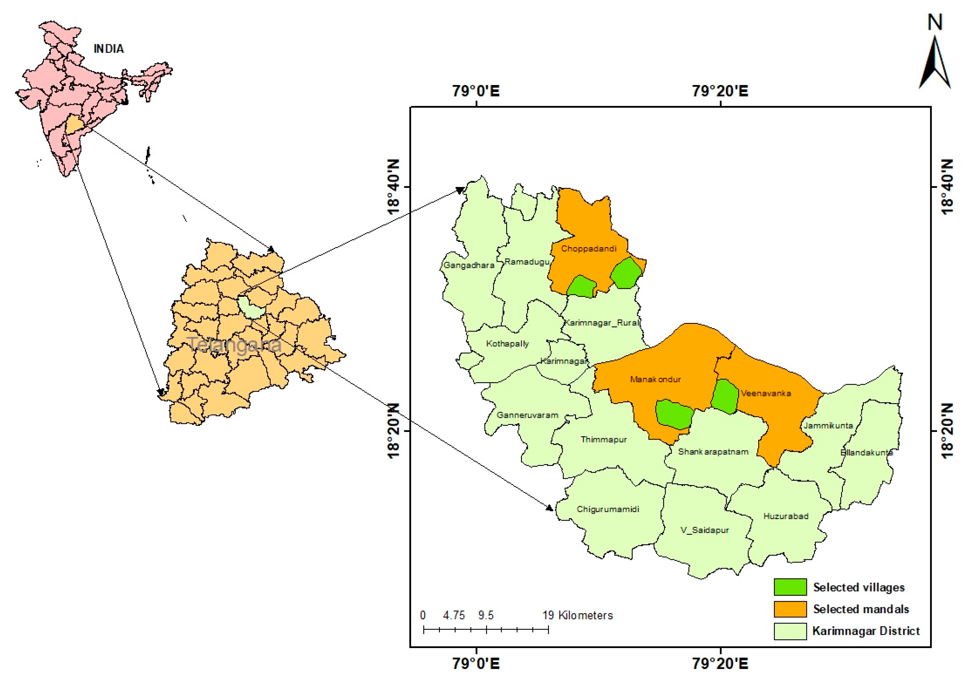
2.1. Study Area
2.2. Methodology for Optimizing Ground Data Points
2.3. Data Used
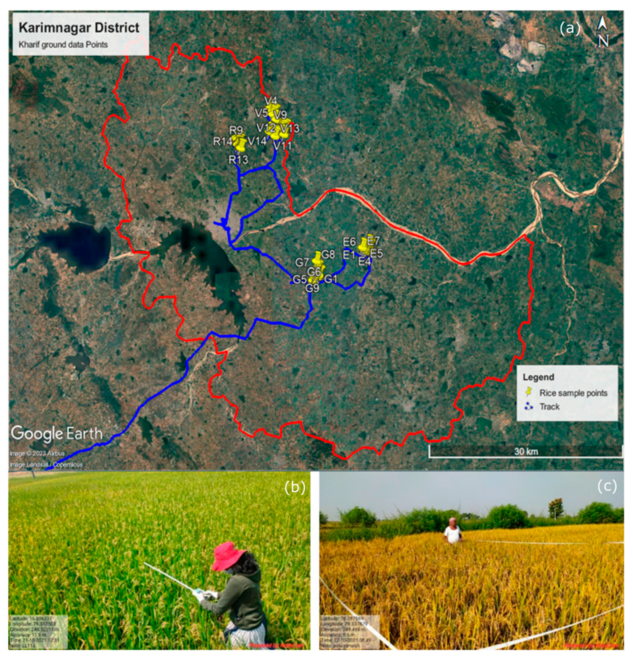
2.4. Ground Data Collection
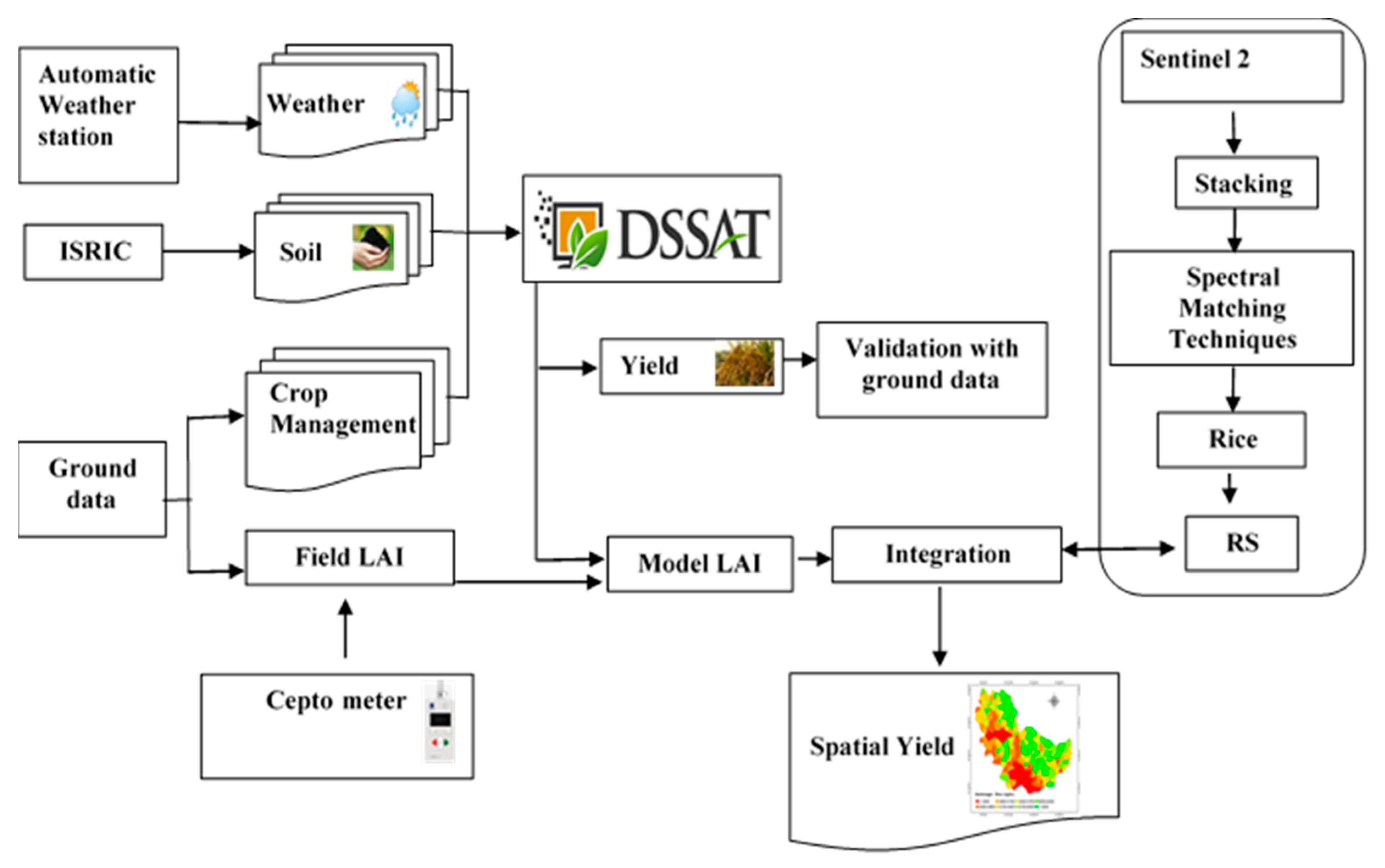
2.5. Crop Model—DSSAT
2.5.1. Weather Data
2.5.2. Soil Data
2.5.3. Crop Management
2.6. Statistical Analysis
3. Results
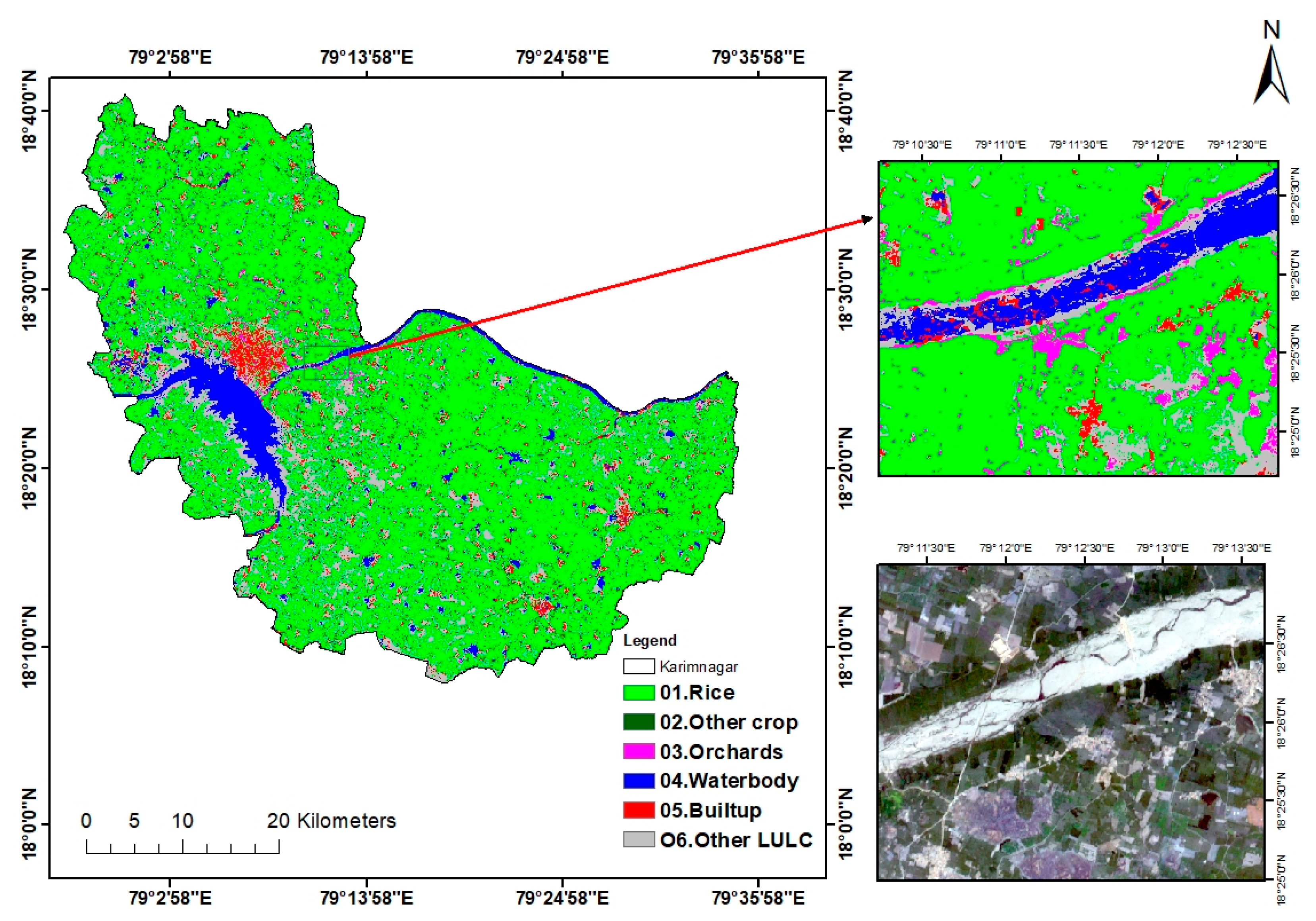
3.1. Classification
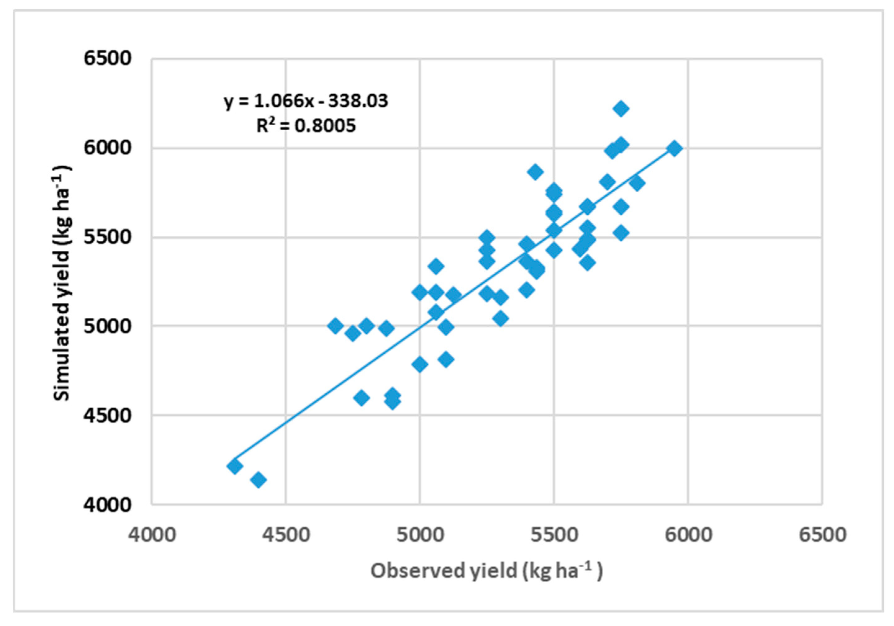
3.2. Model Outputs: Grain Yield
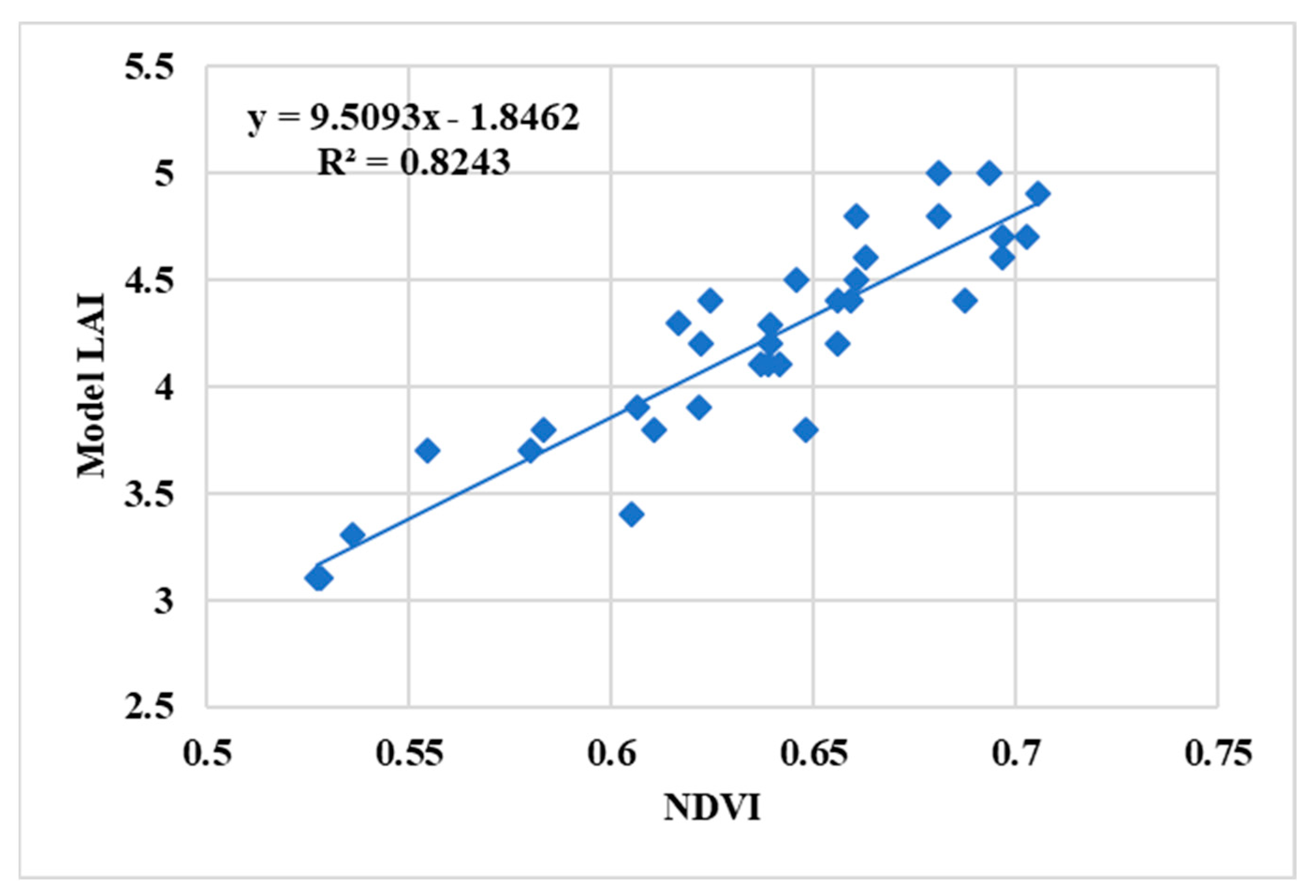
3.3. Integration of Model LAI and Remote Sensing Product
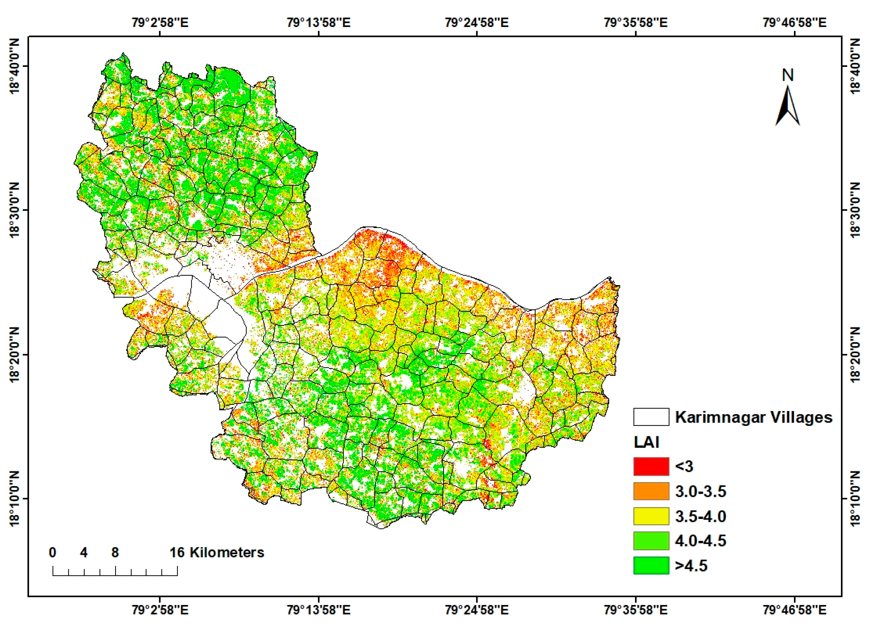
3.4. Generation of Spatial LAI
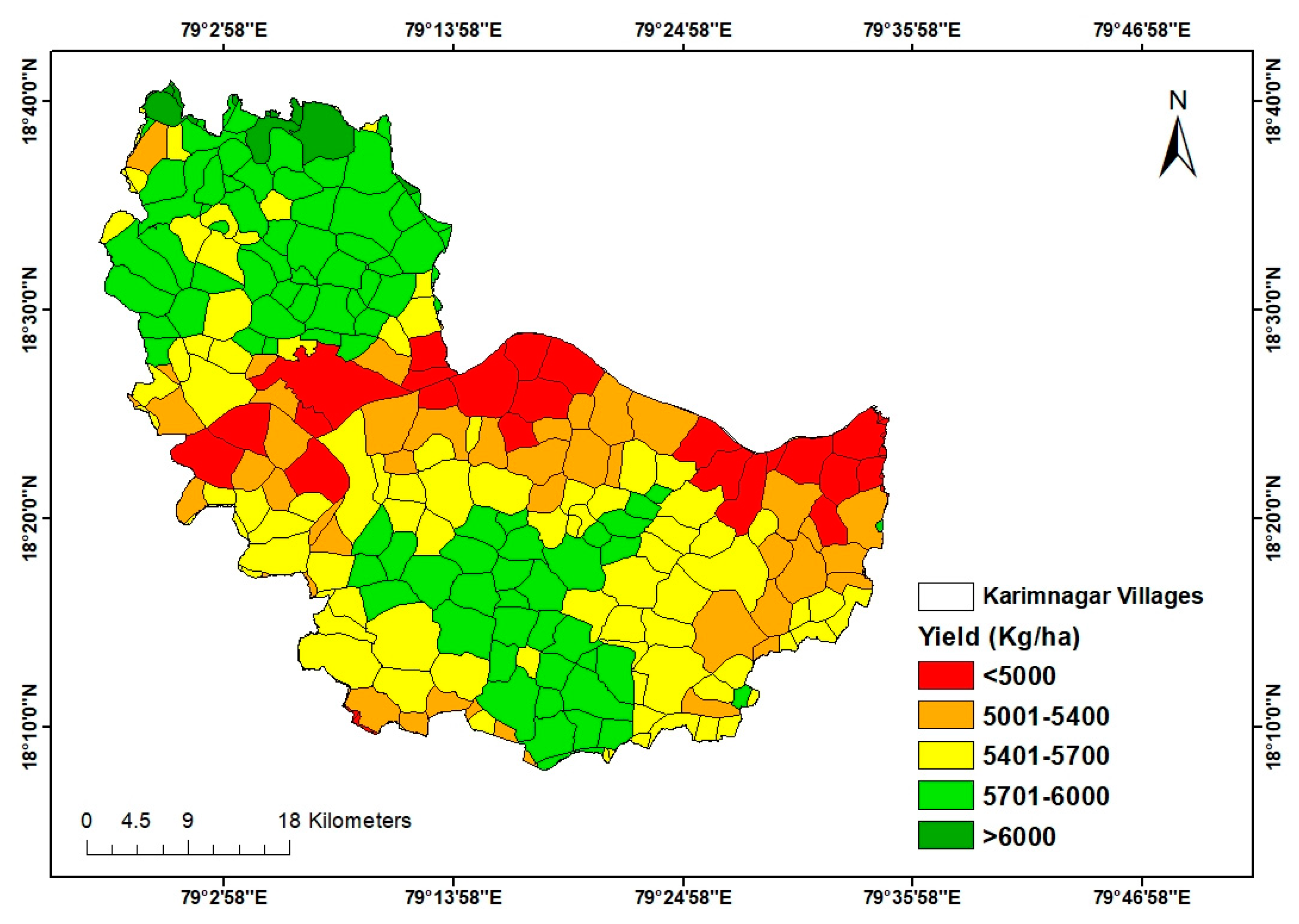
3.5. Generation of Spatial Rice Yield Map
4. Discussion
5. Conclusions
6. Future Line of Work
Author Contributions
Funding
Informed Consent Statement
Data Availability Statement
Acknowledgments
Conflicts of Interest
Appendix A

| Farmer details Name and address Contact no. |
| Location of Plot |
| Area of land holding |
| Previous crop sown |
| Soil type |
| Soil nutrient status |
| Variety name and duration |
| Date of transplanting/sowing |
| Irrigation details No. of irrigations Stages of irrigation |
| Fertilizer details Rate of application Stage of application with quantity |
| Organic amendments (if any applied) |
| Pest and disease attack (if any) Name and quantity of insecticides/pesticides used |
| Date of harvesting |
| Yield (Kg/ha) |
| Soil health card details |
References
- Ahmad, T.; Sahoo, P.M.; Biswas, A.; Singh, D.; Kumar, R.; Basak, P. Agricultural Research Data Book; ICAR Research Data Repository for Knowledge Management: New Delhi, India, 2019.
- U.S. Department of Agriculture. FY 2021 Performance Report; U.S. Department of Agriculture: Washington, DC, USA, 2021.
- Stuart, A.M.; Pame, A.R.P.; Silva, J.V.; Dikitanan, R.C.; Rutsaert, P.; Malabayabas, A.J.B.; Lampayan, R.M.; Radanielson, A.M.; Singleton, G.R. Yield gaps in rice-based farming systems: Insights from local studies and prospects for future analysis. Field Crops Res. 2016, 194, 43–56. [Google Scholar] [CrossRef]
- Government of Telangana. Season and Crop Covergae Report Vanakalam—2021; Report 2021; Government of Telangana: Hyderabad, India, 2021.
- Akula, M.; Bandumula, N.; Rathod, S. Rice production in Telangana: Growth, instability and decomposition analysis. ORYZA-Int. J. Rice 2022, 59, 232–240. [Google Scholar] [CrossRef]
- Basso, B.; Cammarano, D.; Carfagna, E. Review of crop yield forecasting methods and early warning systems. In Proceedings of the First Meeting of the Scientific Advisory Committee of the Global Strategy to Improve Agricultural and Rural Statistics, Rome, Italy, 23–26 February 2013. [Google Scholar]
- Masson-Delmotte, V.; Zhai, P.; Pörtner, H.-O.; Roberts, D.; Skea, J.; Shukla, P.R.; Pirani, A.; Moufouma-Okia, W.; Péan, C.; Pidcock, R. Global Warming of 1.5 °C; An IPCC Special Report on the impacts of global warming; IPCC: Geneva, Switzerland, 2018; Volume 1, pp. 43–50.
- Zhao, Y.; Potgieter, A.B.; Zhang, M.; Wu, B.; Hammer, G.L. Predicting wheat yield at the field scale by combining high-resolution Sentinel-2 satellite imagery and crop modelling. Remote Sens. 2020, 12, 1024. [Google Scholar] [CrossRef]
- Shanmugapriya, P.; Rathika, S.; Ramesh, T.; Janaki, P. Applications of remote sensing in agriculture-A Review. Int. J. Curr. Microbiol. Appl. Sci 2019, 8, 2270–2283. [Google Scholar] [CrossRef]
- Gumma, M.K.; Nelson, A.; Thenkabail, P.S.; Singh, A.N. Mapping rice areas of South Asia using MODIS multitemporal data. J. Appl. Remote Sens. 2011, 5, 053547. [Google Scholar] [CrossRef]
- Panjala, P.; Gumma, M.K.; Teluguntla, P. Machine Learning Approaches and Sentinel-2 Data in Crop Type Mapping. In Data Science in Agriculture and Natural Resource Management; Springer: Berlin/Heidelberg, Germany, 2022; pp. 161–180. [Google Scholar]
- Bazzi, H.; Baghdadi, N.; El Hajj, M.; Zribi, M.; Minh, D.H.; Ndikumana, E.; Courault, D.; Belhouchette, H. Mapping paddy rice using Sentinel-1 SAR time series in Camargue, France. Remote Sens. 2019, 11, 887. [Google Scholar] [CrossRef]
- Rwanga, S.S.; Ndambuki, J.M. Accuracy assessment of land use/land cover classification using remote sensing and GIS. Int. J. Geosci. 2017, 8, 611. [Google Scholar] [CrossRef]
- Jog, S.; Dixit, M. Supervised classification of satellite images. In Proceedings of the 2016 Conference on Advances in Signal Processing (CASP), Pune, India, 9–11 June 2016; IEEE: Piscataway, NJ, USA, 2016. [Google Scholar]
- Gumma, M.K.; Thenkabail, P.S.; Deevi, K.C.; Mohammed, I.A.; Teluguntla, P.; Oliphant, A.; Xiong, J.; Aye, T.; Whitbread, A.M. Mapping cropland fallow areas in myanmar to scale up sustainable intensification of pulse crops in the farming system. GIScience Remote Sens. 2018, 55, 926–949. [Google Scholar] [CrossRef]
- Blackmore, S. The Role of Yield Maps in Precision Farming. Ph.D. Thesis, Cranfield University, Cranfield, UK, 2003. [Google Scholar]
- Griffin, T.W.; Lowenberg-DeBoer, J.; Lambert, D.M.; Peone, J.; Payne, T.; Daberkow, S.G. Adoption, Profitability, and Making Better Use of Precision Farming Data; Department of Agricultural Economics Purdue University: West Lafayette, IN, USA, 2004. [Google Scholar]
- Hajjarpoor, A.; Vadez, V.; Soltani, A.; Gaur, P.; Whitbread, A.; Babu, D.S.; Gumma, M.K.; Diancoumba, M.; Kholová, J. Characterization of the main chickpea cropping systems in India using a yield gap analysis approach. Field Crops Res. 2018, 223, 93–104. [Google Scholar] [CrossRef]
- Mottaleb, K.A.; Gumma, M.K.; Mishra, A.K.; Mohanty, S. Quantifying production losses due to drought and submergence of rainfed rice at the household level using remotely sensed MODIS data. Agric. Syst. 2015, 137, 227–235. [Google Scholar] [CrossRef]
- Hatfield, J.L.; Prueger, J.H. Value of using different vegetative indices to quantify agricultural crop characteristics at different growth stages under varying management practices. Remote Sens. 2010, 2, 562–578. [Google Scholar] [CrossRef]
- Militino, A.F.; Ugarte, M.D.; Pérez-Goya, U. Stochastic spatio-temporal models for analysing NDVI distribution of GIMMS NDVI3g images. Remote Sens. 2017, 9, 76. [Google Scholar] [CrossRef]
- Watson, J.; Challinor, A.J.; Fricker, T.E.; Ferro, C.A. Comparing the effects of calibration and climate errors on a statistical crop model and a process-based crop model. Clim. Change 2015, 132, 93–109. [Google Scholar] [CrossRef]
- Lobell, D.B.; Field, C.B.; Cahill, K.N.; Bonfils, C. Impacts of future climate change on California perennial crop yields: Model projections with climate and crop uncertainties. Agric. For. Meteorol. 2006, 141, 208–218. [Google Scholar] [CrossRef]
- Gumma, M.K.; Kadiyala, M.; Panjala, P.; Ray, S.S.; Akuraju, V.R.; Dubey, S.; Smith, A.P.; Das, R.; Whitbread, A.M. Assimilation of remote sensing data into crop growth model for yield estimation: A case study from India. J. Indian Soc. Remote Sens. 2022, 50, 257–270. [Google Scholar] [CrossRef]
- Sarkar, R.; Kar, S. Evaluation of management strategies for sustainable rice–wheat cropping system, using DSSAT seasonal analysis. J. Agric. Sci. 2006, 144, 421–434. [Google Scholar] [CrossRef]
- Timsina, J.; Humphreys, E. Performance of CERES-Rice and CERES-Wheat models in rice–wheat systems: A review. Agric. Syst. 2006, 90, 5–31. [Google Scholar] [CrossRef]
- O’Neal, M.R.; Frankenberger, J.R.; Ess, D.R. Use of CERES-Maize to study effect of spatial precipitation variability on yield. Agric. Syst. 2002, 73, 205–225. [Google Scholar] [CrossRef]
- Behera, S.; Panda, R. Integrated management of irrigation water and fertilizers for wheat crop using field experiments and simulation modeling. Agric. Water Manag. 2009, 96, 1532–1540. [Google Scholar] [CrossRef]
- Liu, H.; Yang, J.; Drury, C.a.; Reynolds, W.; Tan, C.; Bai, Y.; He, P.; Jin, J.; Hoogenboom, G. Using the DSSAT-CERES-Maize model to simulate crop yield and nitrogen cycling in fields under long-term continuous maize production. Nutr. Cycl. Agroecosystems 2011, 89, 313–328. [Google Scholar] [CrossRef]
- Singh, P.; Singh, K.; Baxla, A.; Rathore, L. Impact of climatic variability on wheat yield predication using DSSAT v 4.5 (CERES-wheat) model for the different agroclimatic zones in India. In Climate Change Modelling, Planning and Policy for Agriculture; Springer: Berlin/Heidelberg, Germany, 2015; pp. 45–55. [Google Scholar]
- Balderama, O.; Alejo, L.; Tongson, E. Calibration, validation and application of CERES-Maize model for climate change impact assessment in Abuan Watershed, Isabela, Philippines. Clim. Disaster Dev. J. 2016, 2, 11–20. [Google Scholar] [CrossRef]
- Doraiswamy, P.C.; Moulin, S.; Cook, P.W.; Stern, A. Crop yield assessment from remote sensing. Photogramm. Eng. Remote Sens. 2003, 69, 665–674. [Google Scholar] [CrossRef]
- Parker, G.G. Tamm review: Leaf Area Index (LAI) is both a determinant and a consequence of important processes in vegetation canopies. For. Ecol. Manag. 2020, 477, 118496. [Google Scholar] [CrossRef]
- Yan, G.; Hu, R.; Luo, J.; Weiss, M.; Jiang, H.; Mu, X.; Xie, D.; Zhang, W. Review of indirect optical measurements of leaf area index: Recent advances, challenges, and perspectives. Agric. For. Meteorol. 2019, 265, 390–411. [Google Scholar] [CrossRef]
- Ren, H.; Liu, R.; Yan, G.; Mu, X.; Li, Z.-L.; Nerry, F.; Liu, Q. Angular normalization of land surface temperature and emissivity using multiangular middle and thermal infrared data. IEEE Trans. Geosci. Remote Sens. 2014, 52, 4913–4931. [Google Scholar]
- Yu, Y.; Wang, J.; Liu, G.; Cheng, F. Forest leaf area index inversion based on landsat OLI data in the Shangri-La City. J. Indian Soc. Remote Sens. 2019, 47, 967–976. [Google Scholar] [CrossRef]
- Hui, J.; Yao, L. A method to upscale the Leaf Area Index (LAI) using GF-1 data with the assistance of MODIS products in the Poyang Lake watershed. J. Indian Soc. Remote Sens. 2018, 46, 551–560. [Google Scholar] [CrossRef]
- Dorigo, W.A.; Zurita-Milla, R.; de Wit, A.J.; Brazile, J.; Singh, R.; Schaepman, M.E. A review on reflective remote sensing and data assimilation techniques for enhanced agroecosystem modeling. Int. J. Appl. Earth Obs. Geoinf. 2007, 9, 165–193. [Google Scholar] [CrossRef]
- Hatfield, J.; Asrar, G.; Kanemasu, E.T. Intercepted photosynthetically active radiation estimated by spectral reflectance. Remote Sens. Environ. 1984, 14, 65–75. [Google Scholar] [CrossRef]
- Wiegand, C.; Maas, S.; Aase, J.; Hatfield, J.; Pinter Jr, P.; Jackson, R.; Kanemasu, E.; Lapitan, R. Multisite analyses of spectral-biophysical data for wheat. Remote Sens. Environ. 1992, 42, 1–21. [Google Scholar] [CrossRef]
- Batchelor, W.D.; Basso, B.; Paz, J.O. Examples of strategies to analyze spatial and temporal yield variability using crop models. Eur. J. Agron. 2002, 18, 141–158. [Google Scholar] [CrossRef]
- Thenkabail, P.S.; Stucky, N.; Griscom, B.W.; Ashton, M.S.; Diels, J.; Van der Meer, B.; Enclona, E. Biomass estimations and carbon stock calculations in the oil palm plantations of African derived savannas using IKONOS data. Int. J. Remote Sens. 2004, 25, 5447–5472. [Google Scholar] [CrossRef]
- Gumma, M.K.; Thenkabail, P.S.; Teluguntla, P.; Rao, M.N.; Mohammed, I.A.; Whitbread, A.M. Mapping rice-fallow cropland areas for short-season grain legumes intensification in South Asia using MODIS 250 m time-series data. Int. J. Digit. Earth 2016, 9, 981–1003. [Google Scholar] [CrossRef]
- Thenkabail, P.; GangadharaRao, P.; Biggs, T.; Krishna, M.; Turral, H. Spectral matching techniques to determine historical land-use/land-cover (LULC) and irrigated areas using time-series 0.1-degree AVHRR pathfinder datasets. Photogramm. Eng. Remote Sens. 2007, 73, 1029–1040. [Google Scholar]
- Jones, J.W.; Hoogenboom, G.; Porter, C.H.; Boote, K.J.; Batchelor, W.D.; Hunt, L.; Wilkens, P.W.; Singh, U.; Gijsman, A.J.; Ritchie, J.T. The DSSAT cropping system model. Eur. J. Agron. 2003, 18, 235–265. [Google Scholar] [CrossRef]
- Hargreaves, G.; Samani, Z. Reference crop evapotranspiration from ambient air temperature. In Proceedings of the American Society of Agricultural Engineers Meeting, Chicago, IL, USA, 17 December 1985. [Google Scholar]
- Ritchie, J.T. Model for predicting evaporation from a row crop with incomplete cover. Water Resour. Res. 1972, 8, 1204–1213. [Google Scholar] [CrossRef]
- Batjes, N. ISRIC-WISE Global Data Set of Derived Soil Properties on a 0.5 by 0.5 Degree Grid (Version 3.0); ISRIC—World Soil Information: Wageningen, The Netherlands, 2005. [Google Scholar]
- Willmott, C.J.; Ackleson, S.G.; Davis, R.E.; Feddema, J.J.; Klink, K.M.; Legates, D.R.; O’donnell, J.; Rowe, C.M. Statistics for the evaluation and comparison of models. J. Geophys. Res. Oceans 1985, 90, 8995–9005. [Google Scholar] [CrossRef]
- Garnier, P.; Neel, C.; Mary, B.; Lafolie, F. Evaluation of a nitrogen transport and transformation model in a bare soil. Eur. J. Soil Sci. 2001, 52, 253–268. [Google Scholar] [CrossRef]
- Fan, L.-y.; Gao, Y.-z.; Brück, H.; Bernhofer, C. Investigating the relationship between NDVI and LAI in semi-arid grassland in Inner Mongolia using in-situ measurements. Theor. Appl. Climatol. 2009, 95, 151–156. [Google Scholar] [CrossRef]
- Goswami, S.; Gamon, J.; Vargas, S.; Tweedie, C. Relationships of NDVI, Biomass, and Leaf Area Index (LAI) for six key plant species in Barrow, Alaska. PeerJ Prepr. 2015, 3, e913v1. [Google Scholar]
- Bhanusree, D.; Srinivasachary, D.; Nirmala, B.; Supriya, K.; Naik, B.B.; Rathod, S.; Brajendra; Reddy, B.N.K.; Bellamkonda, J. Application of the CERES-Rice Model for Rice Yield Gap Analysis. Int. J. Environ. Clim. Change 2022, 12, 3471–3478. [Google Scholar] [CrossRef]
- Maki, M.; Sekiguchi, K.; Homma, K.; Hirooka, Y.; Oki, K. Estimation of rice yield by SIMRIW-RS, a model that integrates remote sensing data into a crop growth model. J. Agric. Meteorol. 2017, 73, 2–8. [Google Scholar] [CrossRef]
- Son, N.; Chen, C.; Chen, C.; Chang, L.; Chiang, S. Rice yield estimation through assimilating satellite data into a crop simumlation model. The Int. Arch. Photogramm. Remote Sens. Spat. Inf. Sci. 2016, 41, 993–996. [Google Scholar] [CrossRef]
- Pazhanivelan, S.; Geethalakshmi, V.; Tamilmounika, R.; Sudarmanian, N.; Kaliaperumal, R.; Ramalingam, K.; Sivamurugan, A.; Mrunalini, K.; Yadav, M.K.; Quicho, E.D. Spatial rice yield estimation using multiple linear regression analysis, semi-physical approach and assimilating SAR satellite derived products with DSSAT crop simulation model. Agronomy 2022, 12, 2008. [Google Scholar] [CrossRef]


| Satellite Imagery | Band | Significance |
|---|---|---|
| Sentinel-2 | B4 (Red) | Helps in recognizing the difference between vegetation and other classes |
| B8 (NIR) | Helps in identifying Water and vegetation | |
| NDVI | (B8–B4)/B8 + B4 | Identifies greenness. (vegetation identification) |
| Classified Data | Producer’s Accuracy (%) | User’s Accuracy (%) |
|---|---|---|
| Rice | 95.96 | 96.94 |
| Another crop | 85.71 | 85.71 |
| Waterbody | 100 | 100 |
| Orchards | 87.50 | 87.50 |
| Built-up | 85.71 | 100 |
| Other LULC | 83.33 | 71.43 |
| Overall Accuracy | 93.04% | |
| Kappa Coefficient | 0.87 | |
| Village Name | R2 | RMSE | D-Index |
|---|---|---|---|
| Elbaka | 0.80 | 374 | 0.86 |
| Gangipalle | 0.87 | 238 | 0.93 |
| Rukmapur | 0.76 | 400 | 0.73 |
| Vedurugattu | 0.72 | 270 | 0.88 |
Disclaimer/Publisher’s Note: The statements, opinions and data contained in all publications are solely those of the individual author(s) and contributor(s) and not of MDPI and/or the editor(s). MDPI and/or the editor(s) disclaim responsibility for any injury to people or property resulting from any ideas, methods, instructions or products referred to in the content. |
© 2023 by the authors. Licensee MDPI, Basel, Switzerland. This article is an open access article distributed under the terms and conditions of the Creative Commons Attribution (CC BY) license (https://creativecommons.org/licenses/by/4.0/).
Share and Cite
Mandapati, R.; Gumma, M.K.; Metuku, D.R.; Bellam, P.K.; Panjala, P.; Maitra, S.; Maila, N. Crop Yield Assessment Using Field-Based Data and Crop Models at the Village Level: A Case Study on a Homogeneous Rice Area in Telangana, India. AgriEngineering 2023, 5, 1909-1924. https://doi.org/10.3390/agriengineering5040117
Mandapati R, Gumma MK, Metuku DR, Bellam PK, Panjala P, Maitra S, Maila N. Crop Yield Assessment Using Field-Based Data and Crop Models at the Village Level: A Case Study on a Homogeneous Rice Area in Telangana, India. AgriEngineering. 2023; 5(4):1909-1924. https://doi.org/10.3390/agriengineering5040117
Chicago/Turabian StyleMandapati, Roja, Murali Krishna Gumma, Devender Reddy Metuku, Pavan Kumar Bellam, Pranay Panjala, Sagar Maitra, and Nagaraju Maila. 2023. "Crop Yield Assessment Using Field-Based Data and Crop Models at the Village Level: A Case Study on a Homogeneous Rice Area in Telangana, India" AgriEngineering 5, no. 4: 1909-1924. https://doi.org/10.3390/agriengineering5040117