

Video Compression Prototype for Autonomous Vehicles

Computer Science Department, Bar-Ilan University, Ramat Gan 5290002, Israel
Smart Cities 2024, 7(2), 758-771; https://doi.org/10.3390/smartcities7020031
Submission received: 23 November 2023
/
Revised: 5 March 2024
/
Accepted: 6 March 2024
/
Published: 8 March 2024
(This article belongs to the Topic Advanced Array Signal Processing for B5G/6G: Models, Algorithms, and Applications)
Abstract
:There are several standards for representing and compressing video information. These standards are adapted to the vision of the human eye. Autonomous cars see and perceive objects in a different way than humans and, therefore, the common standards are not suitable for them. In this paper, we will present a way of adjusting the common standards to be appropriate for the vision of autonomous cars. The focus of this paper will be on the H.264 format, but a similar order can be adapted to other standards as well.
1. Introduction
Autonomous vehicles [1] make use of videos and not just still images, for two main reasons:
- It is necessary to transfer different types of information, and not all types of information can be transferred in a still image [2]; for example, the direction of drive can be figured out from a video but not from a still image. Speed is also information that can be figured out from video and not from a still image.
- The presentation of the data in the form of a video is actually also a backup of the data, because every frame in the video is similar to the frames nearby, and, so, if one frame is damaged or even disappears completely, there are still the neighboring frames that can cover the loss. There is a limit to the loss that can be absorbed; however, if there are only small deficiencies scattered about, they can certainly be overcome [3].
Video representation methods try to compress the amount of information that needs to be transferred as much as possible while damaging the quality of the information as little as possible. In real-time systems, the necessity for significant compression is clearly greater [4].
Autonomous vehicles are certainly real-time systems. Therefore, the need to improve data compression is important for them. However, when planning an improvement to the video data compression of autonomous vehicles, it must be taken into account that the improvement is for information that passes between computer systems and not information intended for the human eye.
All compression methods for video are methods that intentionally lose some of the information before sending [5]. Some information is omitted completely, and some information is rounded to other numbers with the aim of improving the compression quality.
The decision as to which information should be discarded was made by the developers of the compression methods on the assumption that the goal is to transmit a video that people will watch later; therefore the conventional methods omit information that the human eye is not sensitive to or at least almost not sensitive to, but when it comes to autonomous cars, the considerations have to be different because the systems of autonomous cars are very different from the functioning of the visual systems of humans [6].
When designing video compression for autonomous vehicles, there are several constraints that have to be considered:
- Autonomous vehicles have to be capable of compressing the video information in real time with the aim of making timely decisions.
- Autonomous vehicles have to be capable of transmitting the video information to its destination with the smallest possible delay.
- Various environments should be taken into account which means that a variety of noises and instabilities can occur, and the compression method should be able to recover from them as quickly as possible with minimal information loss.
Autonomous vehicles are in their initial steps; however, it is beyond dispute that they have a substantial ability to advance transportation safety and efficiency. As this technology becomes more integrated into our lives, the use of videos for autonomous vehicles is anticipated to grow significantly. The algorithm developed in this paper aimed to support the utilization of videos by autonomous vehicles.
2. The H.264 Video Compression Standard
When we want to implement a format for autonomous vehicles, it is better not to invent a completely new format from scratch, but rather use techniques that are already known and established and adapt them to the environment of autonomous vehicles.
With regard to the decision on the preferred specific compression format, H.264 has a number of substantial advantages:
- H.264 enjoys widespread popularity, which means that many devices of many brands that are currently in the automotive industry can and know how to use the H.264 format [7].
- H.264 is a royalty-free compression format. The economic consideration is also a consideration that should be taken into account when trying to put forward for consideration a format for practical and realistic use [8].
- Our previous papers explained the error resilience features of H.264 [9]. H.264 exhibits enhanced robustness to errors compared to older video coding standards due to several key features it incorporates. H.264 divides video data into small packets, facilitating loss concealment techniques when errors occur. Missing packets can be replaced with estimates based on surrounding information, minimizing the visual impact. When spatial prediction is insufficient, neighboring frames can be used to create estimates for missing blocks, minimizing temporal inconsistencies. Furthermore, H.264 is based on the Huffman code [10] that synchronizes itself automatically after errors [11].
The main obstacle to adapting H.264 as a compression format for autonomous vehicles is that H.264 was explicitly designed for the human eye. Therefore, H.264 tries to keep the information that the human eye is sensitive to but omits numerous pieces of information that are unnecessary to the human eye [12]. Our goal in this paper is to keep the important information for the decisions of the autonomous vehicle and omit the information that is not important for these decisions, ignoring the actuality of what is important or unimportant for the human eye.
H.264 saves more information for brightness data in an image. The motivation behind this concept lies in the properties of human vision. Human eyes are less adept at perceiving spatial variations in colors compared to spatial variations in brightness. By leveraging this feature, H.264 does not store the information in the conventional RGB format, where each pixel is assigned values for red, green, and blue components. Instead, the information is stored in the YUV color space [13].
In the YUV color space, each pixel also has three values: Y represents brightness (luminance), and U and V represent color (chrominance) information. By breaking up the information into luminance components and chrominance components, H.264 can take advantage of the reduced sensitivity of a human eye to color variations, bringing about more efficient transmission of video information.
Usually, the 4:2:0 arrangement is used. In this subsampling scheme, the luminance values are all kept, however some of the chrominance values are not. Two chrominance values are placed in the first row of each block, whereas the second row has no chrominance values. To complete the missing values in the decoding, each chrominance value is applied for both the two original columns and the two nearby columns in the row below. The 4:2:0 arrangement effectively reduces the resolution by half without a noticeable impairment [14].
H.264 breaks up the image into square regions, each consisting of eight rows and eight columns of pixels. Then, H.264 utilizes a three-stage approach to encode each block of data in each frame [15]. Firstly, H.264 converts each block of data from the sampling domain to the frequency domain using the Forward Discrete Cosine Transform (FDCT) [16]. The Forward Discrete Cosine Transform (FDCT) is a widespread tool in the field of digital signal processing, mainly in the compression of video, images, and audio. While the FDCT shares similarities with the Discrete Fourier Transform (DFT), it differentiates itself by making use of only the cosine function as its core function. The version of FDCT for H.264 8 × 8 block is defined in Equation (1):
where
- F(u,v) are the values in the frequency domain for the indices u, v.
- f(x,y) are the values in the sampling domain for the indices x, y.
- C(u) = 1/√2 if u is 0; otherwise, C(u) = 1.
- C(v) = 1/√2 if v is 0; otherwise, C(v) = 1.
When u = 0 (the DC component), the value represents the average intensity of this block in the image. In FDCT, this value is treated differently from other frequency values due to its distinctive nature. To ensure energy preservation during the transformation from the sampling space, FDCT uses specific normalization factors. For the DC component, this factor is √8, because the size of the block is 8 × 8. The DC coefficient itself does not have a cosine term in the FDCT formula, because cosine of 0 is 1. Thus, instead, it is represented by a constant term 1/√8, which is ½·1/√2. The ½ of u and the ½ of v are written as ¼ in the beginning of the equation. That is to say, the value 1/√2 for C(u) at u = 0 and for C(v) at v = 0 arises from the specific normalization factor used for the DC component in the FDCT to preserve energy and account for its constant nature.
After the FDCT, H.264 quantizes each value by dividing the values by predetermined factors and then rounding the results to the nearest integer. As a final stage, H.264 applies a variant of Huffman coding to encode the data in the results of the previous stage.
In this paper, we focus on the quantization stage that loses some of the information, because we want to lose other information than what H.264 usually loses. Instead of deciding on losing information according to the sensitivity of the human eye, we will lose information according to the needs of the vision systems of autonomous cars.
3. Reducing the Number of Bits
In order for an autonomous vehicle to be able to make a correct decision, there is no need for a high number of shades. Autonomous vehicles primarily rely on features like object edges, shapes, and motion, not subtle color variations. The former can be identified even with limited color resolution. When making critical decisions, autonomous vehicles prioritize specific visual cues that are essential for safe and accurate navigation. These crucial features include object edges, which define an object’s outline and separate it from the background shapes, which provide fundamental information about the object’s type (e.g., car, pedestrian, traffic sign) and motion, which reveals an object’s movement patterns and intentions. Notably, these vital features can be effectively identified and analyzed even with lower color resolution.
While it might seem intuitive that more colors translate to better understanding, it is not always the case for autonomous vehicles. Increasing the number of shades not only requires more processing power and memory but also introduces the potential for irrelevant details to clutter the decision-making process. By focusing on essential features like edges, shapes, and motion, autonomous vehicles can extract critical information efficiently, even with limited color data. By understanding the importance of relevant features and the ability to identify them with lower resolution, we can create more efficient and streamlined autonomous vehicle systems that make accurate decisions without being bogged down by unnecessary information.
H.264 supports hue accuracy (before compression) of 24 bits. This level of accuracy provides 16 M different colors. In our experiments, we reduced the number of bits to only three, so we only support eight colors. To the human eye, such an image appears to be of low quality, but for the decisions of autonomous vehicles, this will be an absolutely sufficient quality.
The eight colors we choose should be, on the one hand, eight colors that appear a large number of times in the image, but on the other hand, if the eight selected colors are very similar, we will not be able to extract information that will reflect the various objects in the image. That’s why we developed Algorithm 1 that will keep these two principles and give us eight frequent colors that are also sufficiently different from each other.
| Algorithm 1 Find the eight paramount colors | |
| |
| (2) | |
| |
| (3) | |
Δ is known as the Feigenbaum constant [17], where an are discrete values of the bifurcation parameter.
For each of the 28 pairs for which we check the variance, we mark the red, green, and blue values of the first color in the pair as red1, green1, and blue1 and the red, green, and blue values of the second color in the pair as red2, green2, and blue2.
In the worst case, the algorithm has to go through the pixels that exist in the image twice—once when it counts the frequency of appearance of the colors and once when it looks for the most frequent colors. We mark the number of pixels with the letter P.
In addition, the algorithm should sort the colors according to their percentage of appearance frequency in the image. We mark the number of colors present in the image with the letter C.
As we know, the complexity of sorting is O(C·log(C)) [18], and, therefore, the complexity of the whole algorithm is shown in Equation (4):
O(P) + O(C·log(C))
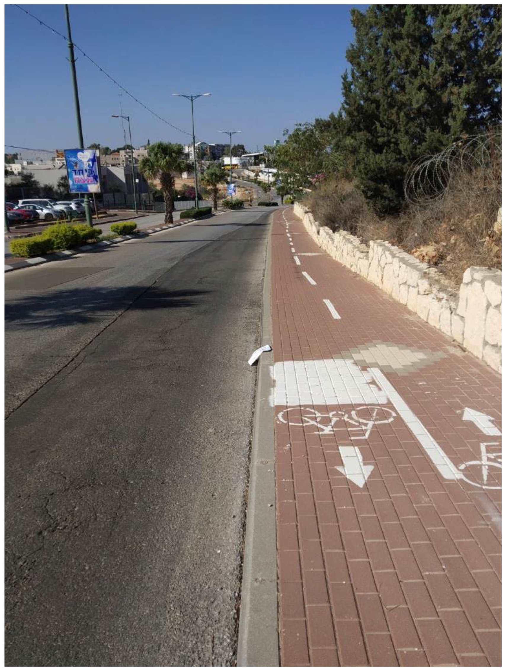
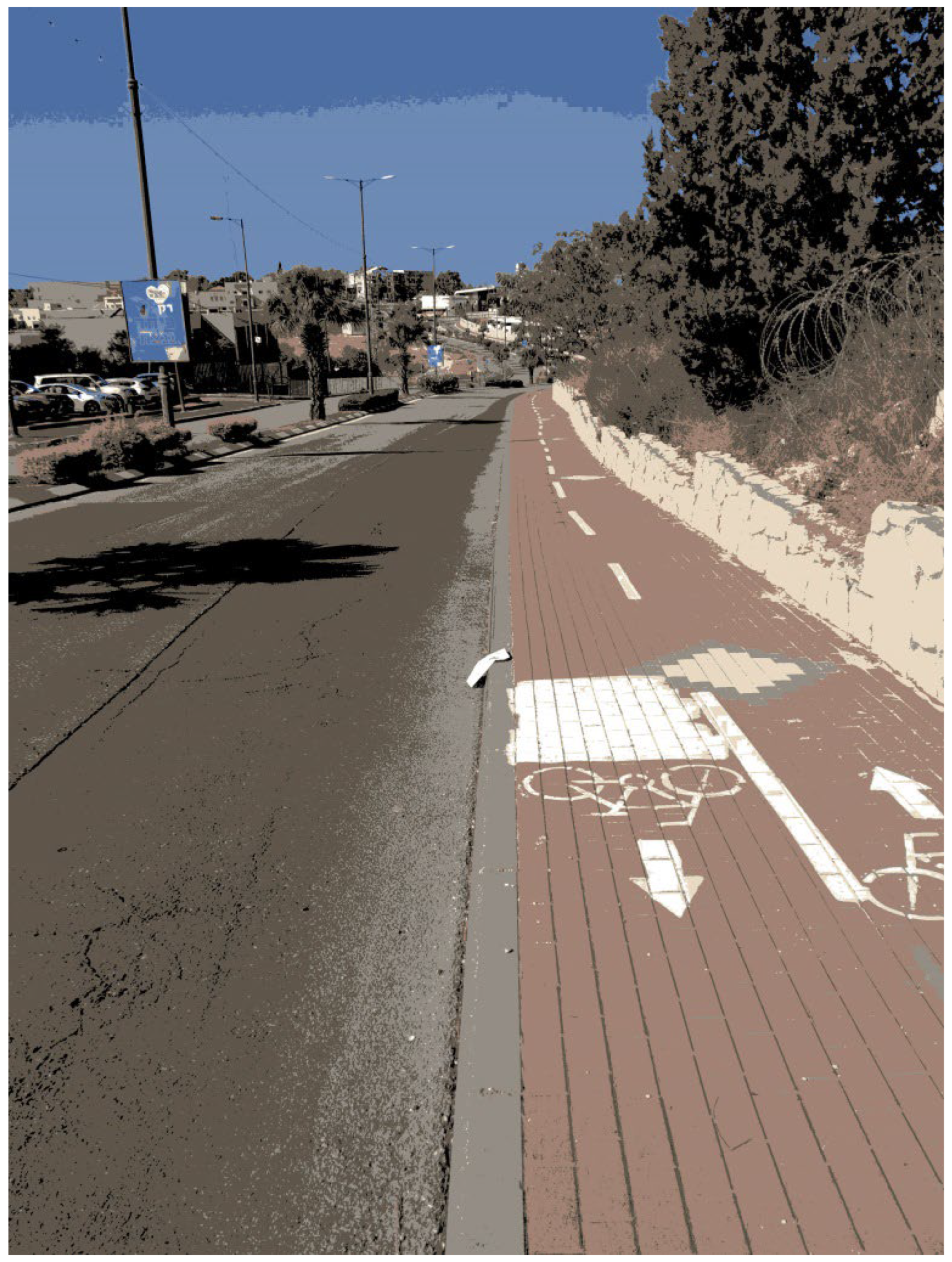
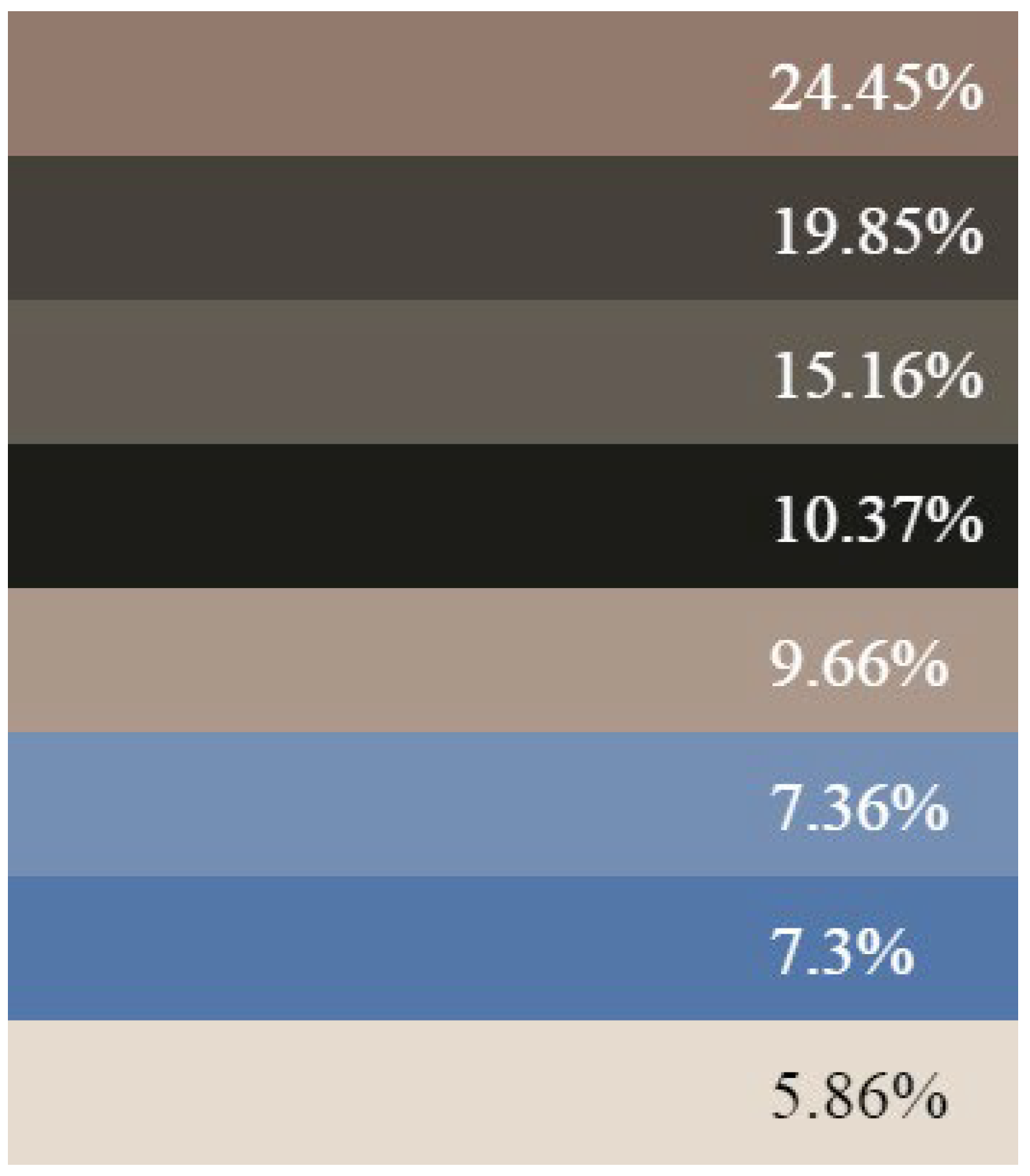
A demonstration of Algorithm 1 is in Figure 1, Figure 2 and Figure 3. Figure 1 shows a picture of a road. We applied the proposed algorithm to this image. In Figure 2, you can see the result of the algorithm—the same image as in Figure 1 with only eight colors. Figure 3 lists the colors selected by the algorithm and their percentages of appearance frequency in the image. The image created as a result of the algorithm is certainly of lower quality; however, even to the human eye the quality is not unbearable, although we can clearly see the differences in several places, such as, for example, in the part of the figure where the trees are.
For autonomous cars, the identification of the boundaries between the various objects, like other vehicles and the identification of road signs and traffic lights, are the aim [19]. For this purpose, reducing the number of colors does not harm the identification; therefore, there is no point and there is no need to save irrelevant information when it comes to the vision of a vehicle and not the vision of a human being. Therefore, a large variety of colors is not required in the vision of autonomous vehicles.
The reduction percentages in the image due to the algorithm are not that high. For example, in this particular image, the original size of the image is 1,479,471 bytes. After reducing the number of colors using the algorithm, the size of the image is reduced to 1,437,773 bytes, which suggests a reduction of only about 2.818%. The reason is that the H.264 format was designed to be suitable for images with gradual changes, i.e., we will receive better compression in images with gradual changes. In the images we created with the algorithm, there are, on the one hand, parts that became completely blank, i.e., without any change; however, on the other hand, there are parts where a gradual change that was in them became a sharp change, like in the part of the image that contains the sky.
Eventually, the improvement in compression in certain parts and the worsening in other parts nearly counterbalance each other, so, as a result, the improvement in compression is very minor. That is why we will propose in the next section a way to modify the quantization tables of H.264 so that the gain from reducing the number of colors will contribute more significant diminution than the loss from merely altering to eight colors that increased the sharp changes in the images.
4. Adapted Quantization Tables for a Small Number of Colors
In the previous step, we reduced the number of possible colors from 16 M to only 8. This reduction creates an incompatibility with the way the H.264 compression format works.
The H.264 format assumes that both the differences between the pixel values and the differences between the frame values are small [20]. In accordance with this assumption, the H.264 quantization tables were built. When we changed the colors, we increased the differences. Many images have a dark pixel, and the transition to a bright pixel is not immediate but gradual. That is, there are pixels with a decreasing degree of darkness as we approach the lightest pixel [21]. Because we decrease the number of colors, the transition becomes sharper and less gradual.
Therefore, depending on the change made in the number of colors, we also need to change the quantization tables to match the data as it is now.
The quantization tables of H.264 are tables that tell by how much to divide the intensity of each frequency that is in the frames’ blocks [22]. The H.264 quantization tables are named after the percentages by which they are expected to compress the frame. That is, if dividing by the values of the quantization tables is expected to give, for example, a compression of 50%, the table will be called “50% quantization table”. Obviously, it is impossible to know exactly for each frame to what percentage of its original size it will be compressed because there are images with large changes and there are images with small changes; however, a general estimate of how much the frame will be compressed can be given, which is why the quantization tables are called that [23].
Autonomous vehicles usually apply a quantization table of 80% to 90% when compressing video using H.264. In some circumstances, autonomous vehicles can apply a quantization table of less than 80% and even 70% or less if they ought to diminish the size of the data even further; however, such a diminution will further decrease the video quality. Indeed, the quantization table of H.264 that autonomous vehicles select to make use of is determined by the application requested by the user and the required quality of video for this application [24].
The results obtained when using our method are quite similar for quantization tables with different percentages. We will present here, as an example, the results for a quantization table of 85%.
In the H.264 standard, after the transition from the sample space to the frequency space, there are 64 frequency values in each block, where each value is represented by two indicators—its frequency on the x-axis and its frequency on the y-axis. The values of the indicators, i.e., the frequencies, range from 0 to 3.5 [25].
The quantization tables consist of 64 coefficients. Each of the coefficients represents the coefficient by which each of the frequency values must be divided. After dividing the frequency values, the result is rounded and, thus, some of the information is lost. Dividing by a larger factor almost always results in greater information loss.
The human eye is much more sensitive to changes in the small frequencies. In addition, when there are minor changes within the blocks, only the small frequencies will have significant values. Therefore, H.264 divides the small frequencies by smaller coefficients to lose less information, whereas H.264 divides the higher frequencies by larger values. In actual fact, H.264 assumes that the small frequencies are the main information and also takes into account that the human eye is more sensitive to them [26].
In our system, the considerations are different, because the system is for vehicle vision and not a human eye, and, in addition, there are more larger changes. Therefore, the standard quantization tables of H.264 are not suitable, and other quantization tables are needed which are suitable for this different type of information.
We make use of the Van der Pauw constant [27,28]. The Van der Pauw constant is used to measure the quality of an object, and we also want to set the quality of the images using the quantization tables.
H.264 quantization tables are employed with the aim of compressing images by decreasing the number of bits required to represent each block. The higher the quality of the quantization table, the finer the quality of the image, but the more space the image will use up. Similarly, the Van der Pauw constant is a physical constant that is employed to evaluate the resistivity of objects. The greater the resistivity of an object, the harder it will be for electricity to flow via that object. Both H.264 quantization tables and the Van der Pauw constant are employed to calculate and determine the quality of an object.
Accordingly, we suggest the formula in Equation (5) for the modified table:
where f(x,y) are the coefficients in the quantization table, K is the Van der Pauw constant, and x, y are the frequencies on the x-axis and the y-axis, respectively.
H.264 quantization tables and optimization algorithms like the Van der Pauw constant share a common goal: achieving desired outcomes with minimal resources. In video compression, quantization tables reduce image data while maintaining quality. Similarly, the Van der Pauw constant helps calculate resistivity efficiently. However, both approaches involve trade-offs: higher quality in H.264 comes with larger file sizes, and the Van der Pauw constant assumes simplified material properties. Understanding these trade-offs is crucial for using these tools effectively. We want there to be differences between the upper left part of the quantization table and the lower right part of this table, but we also want these differences to be smaller than the original ones. To maintain their gradualness, we used the Van der Pauw constant, and, thus, we received, on the one hand, a quantization table with smaller values on the upper left side and, on the other hand, a table that reflects the effectiveness of the trade-off between the different waves created by the FDCT function.
The calculation results of Formula (3) for all 64 coefficient values of the new quantization table produce Table 3:
All the numbers have been rounded to the nearest integer. The original quantization tables also contain only integers, and we would like to maintain compatibility with the original algorithm. As a matter of fact, even so, the level of accuracy is high enough, and adding digits to the right of the decimal dot for the fraction will only slightly increase the accuracy but significantly harm the compression; so, in this feature, we have not changed the policy of H.264.
5. Results
Following the rationales that are true for the human eye explained above, the original H.264 quantization table is constructed so that there are very substantial differences between the upper-left part of the table and the lower-right part of the table. The differences are so large that, for the example in the 85% table we showed above, the values are from 3 to 30; that is a difference of 10 times. According to the formula we propose, there is still a difference, but it is significantly smaller. The values are from 5 to 22, meaning a 4.4-fold difference instead of a 10-fold difference.
In addition, the human eye is much less sensitive to the chrominance component of the image than to the luminance component; therefore, the H.264 standard offers two different tables, one for the chrominance component and one for the luminance component, with the difference between them reflecting the difference between the sensitivity of the human eye and each of the image components [29].
A vehicle’s vision systems do not function like a human eye, and there is no difference between the quality of vehicle’s vision of the chrominance component and the quality of vehicle’s vision of the luminance component. In paper [30], the authors explain that the Image Signal Processor (ISP) steps, including the transformation from RGB components to waves, are designed to provide a high degree of static visual performance to the end user for human viewing applications. This may be unnecessary or even counterproductive for computer vision-based applications. The authors of this paper claim that the standard cameras equally perceive the RGB and YUV components. Then, the software that processes this information works very differently from the way a human brain works, and the information that reaches them from each of the components contributes similarly to their decisions. Human eyes have a complex structure with various components, like the cornea, lens, and retina, allowing for features like color perception, depth perception, and adaptation to varying light conditions. Vehicle vision systems, on the other hand, typically rely on cameras and other sensors that capture and process visual information electronically. They lack the biological and physiological capabilities of the human eye. That is why they perceive reality differently.
Therefore, we used the same table for the chrominance component and the luminance component. Using the recommended quantization table, the size of the picture in Figure 2 (the eight-color picture) was compressed to 1,081,937 bytes, which is 26.87% better than the compression of the original image using the standard 85% quantization table.
The variation in the level of image quality required is according to the level of sharpness of the change in the image. The sharpness of the change is not necessarily in accordance with the nature of the task required of the autonomous vehicle, and, in fact, the relationship between them, is quite doubtful. For example, the sign recognition in Figure 2 differs in its difficulty in different areas. This road sign is blue in color, which resembles the sky, and, therefore, the recognition task is more difficult. On the other hand, there are gray houses on the sign’s sides, so the change is sharper, and, therefore, it is easier to recognize the sign. Similarly, identifying the border between the road and the sidewalk can be of varying degrees of difficulty, because sometimes the edge of the sidewalk is a gray color similar to the road, yet sometimes it is painted white, red, black, or blue. While the required image quality can vary depending on the level of detail needed to detect changes in the image, this detail level may not directly correlate with the specific task an autonomous vehicle needs to perform.
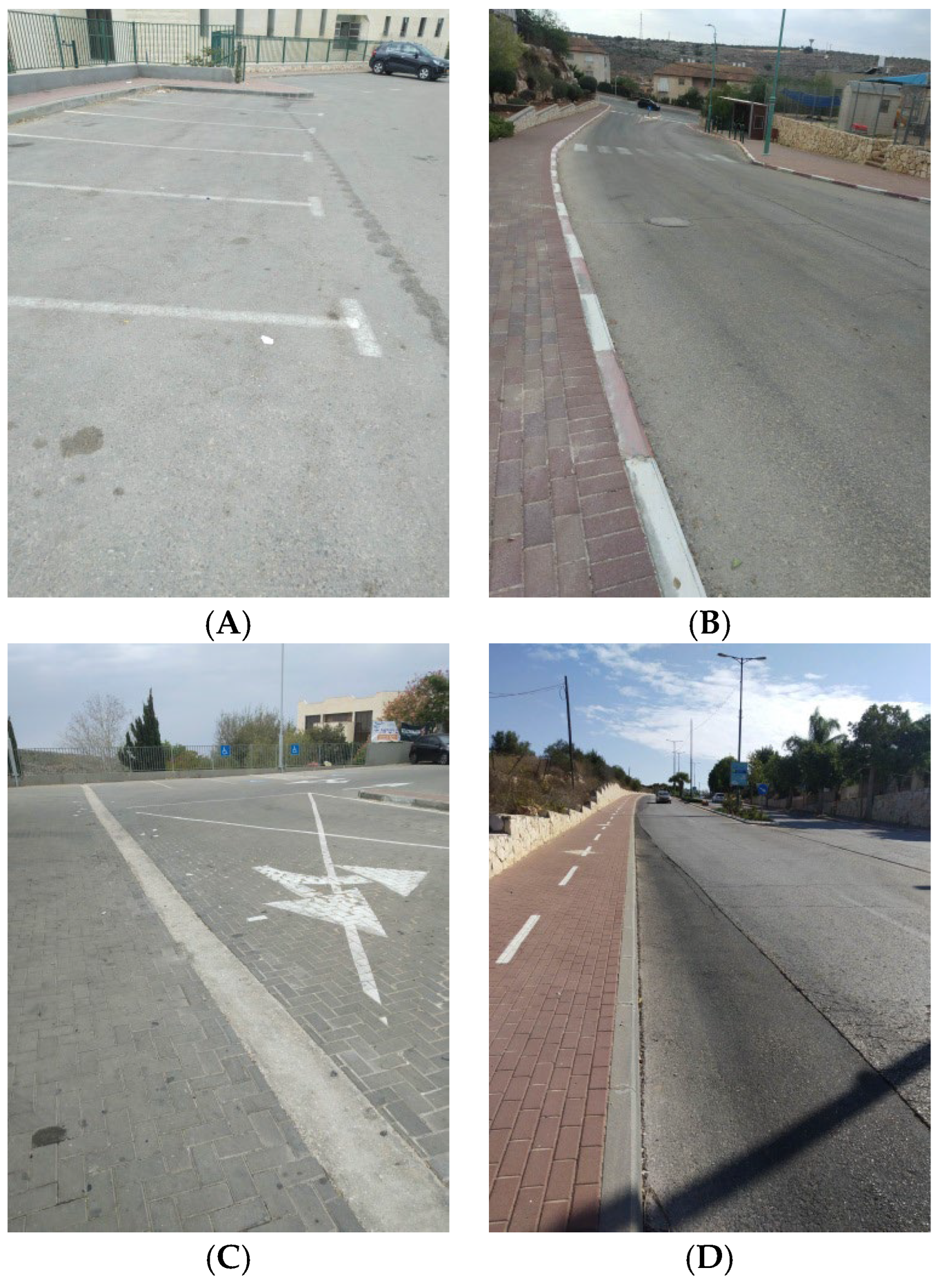
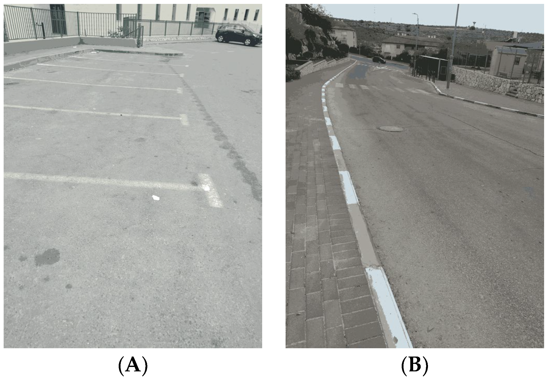
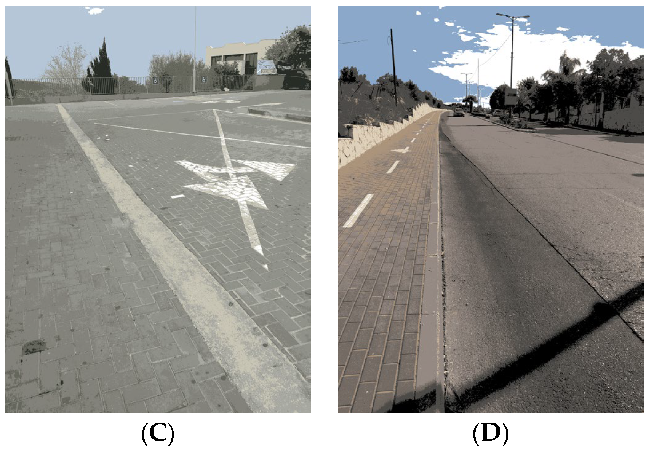
We tested more images to see the effectiveness of the compression. The original images are shown in Figure 4, and the eight-color images are shown in Figure 5. Once again, we made use of the standard quantization tables of 85% for the original images and the quantization table suggested in Figure 3 for the eight-color images.
The images retain their visual appeal despite the presence of some minor quality degradation. The differences are evident in cases where there is a gradual change, such as the cloud found in image D, where there is a gradual transition between white and light blue. The gradual transition becomes a sharp transition between only two colors, white and light blue. Consequently, on the one hand, inside and outside the cloud, there is no change, and the blocks without the changes are effectively compressed by H.264. On the other hand, there are blocks where a sharp change between white and light blue is found, and such a change is ineffectively compressed by H.264 compared to the compression of gradual changes that were in the original image.
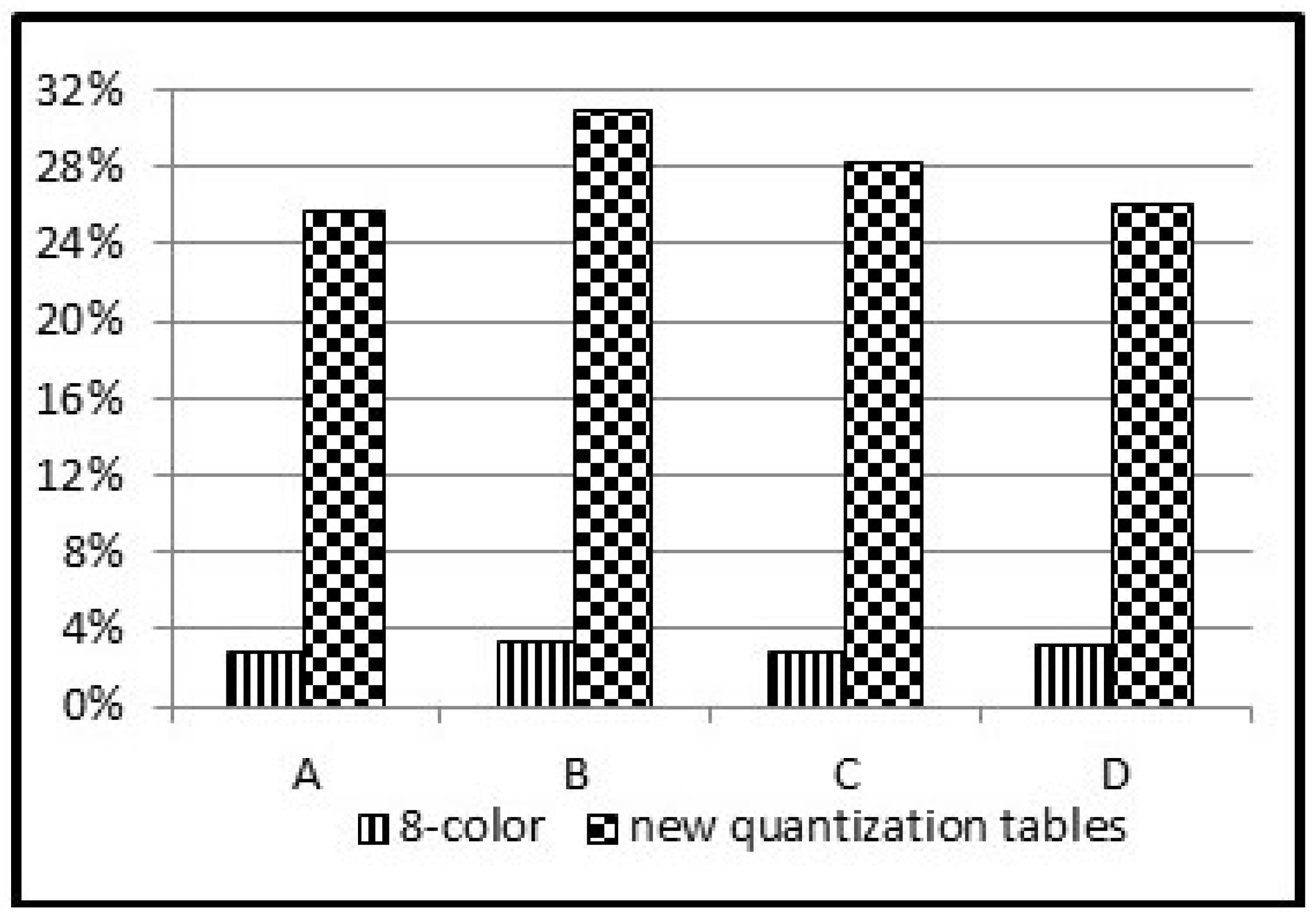
The results are detailed in Figure 6. The left column shows the reduction after the reduction to eight colors. The compression effectiveness of the proposed method. i.e., reduction to eight colors and changing the quantization tables. is shown in the right column.
It can be seen that the results of the compression ratios are quite similar in the various images and show quite a high degree of consistency.
The shift to eight colors can lead to finding a rare color as one of the eight frequent colors. For example, in Figure 5A, most of the colors are quite close to each other, so the algorithm did not select them. In the end, the algorithm chose the eighth most frequent color that appeared in only 1.37% of the image.
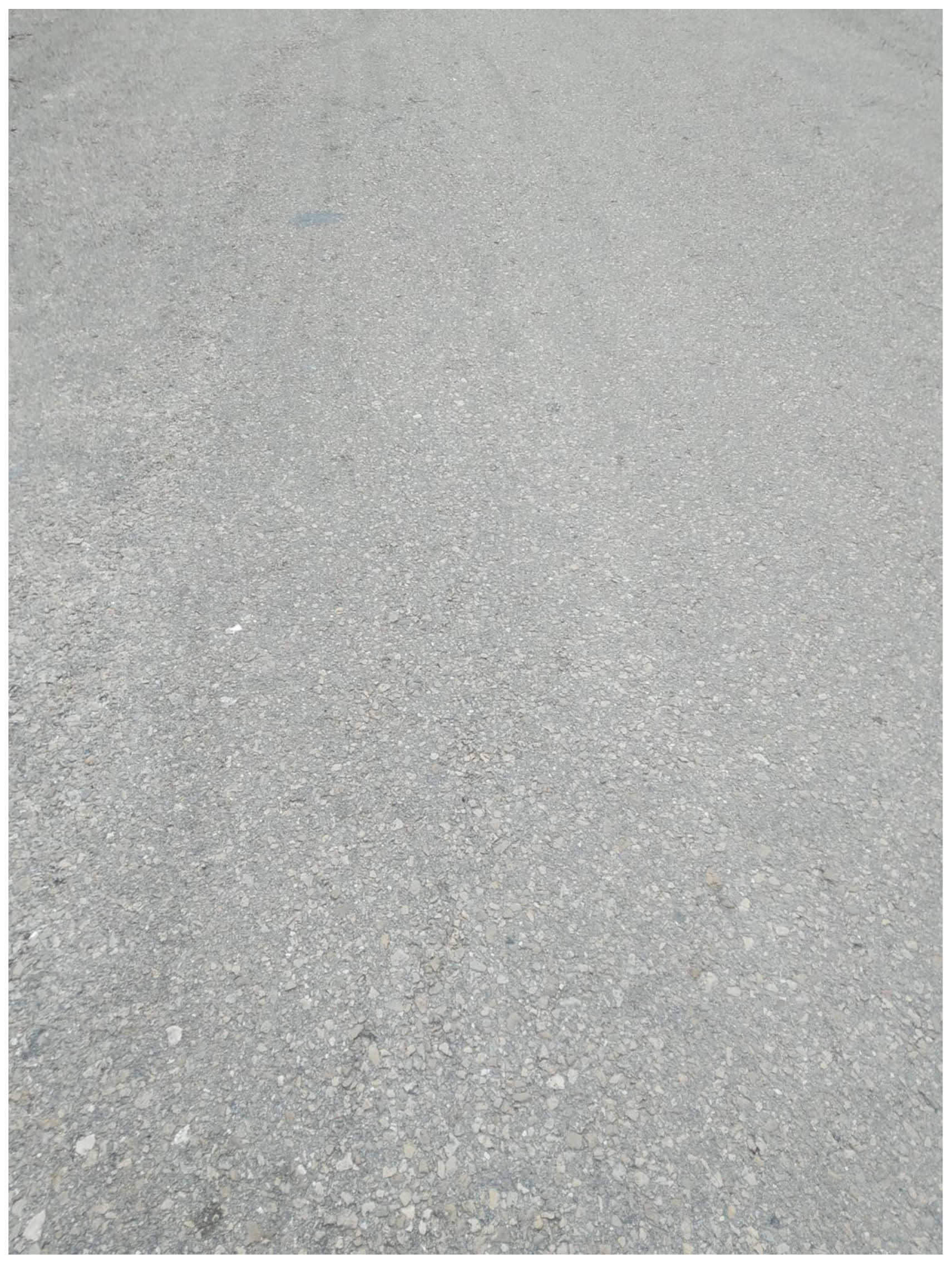
In actual fact, there could even be a situation where there would not be eight colors, because the colors would be too close to each other in their hue. For example, in Figure 7, there are only five shades far enough from each other because the image only contains a picture of an asphalt road. In such cases, the algorithm chooses a smaller number of colors and does not insist on eight colors.
Indeed, switching to a palette of eight colors for image compression presents potential issues when dealing with rare colors. This occurs because the compression algorithm might struggle to differentiate between subtle color variations and even lead, once in a while, to insufficient colors.
In extreme cases, the algorithm might be unable to find eight distinct colors within the image due to their extreme closeness in terms of hue. This scenario leads to the algorithm selecting a smaller number of colors, deviating from the intended eight-color palette. However, contrast and detail are maintained, enabling accurate edge detection despite the color reduction.
6. Conclusions
Almost all videos transmitted over any network are compressed because they contain voluminous data and, therefore, use quite a bit of network bandwidth. The videos used by the autonomous vehicles are often large in size, so they must also be compressed [31].
Since all video compressions omit some of the information, compression algorithms need to know which part of the information can be omitted. The difference between the compression of conventional video and the compression of the video of autonomous vehicles is who looks at the decoded video. There is a difference between the information that can be omitted when the information is for a human eye, and the information that can be omitted when the information is for a component of an autonomous vehicle.
In this paper, we propose to modify the well-known H.264 format, which is intended for video compression that will eventually be seen by a human eye. We suggest reducing the number of colors in the image to only eight and, in addition, as a complementary step, to modify the quantization tables of H.264, so that they match up an image with a small number of colors.
The results look promising. The remaining information is sufficient for autonomous vehicles, and the compression improves by considerable percentages, so the findings are encouraging.
Future research efforts will further ensure that the compressed video retains the information essential for the autonomous vehicle’s perception system to make safe driving decisions. Since video compression for autonomous vehicles prioritizes information critical for safe operation, the quality assessments should go beyond the traditional metrics used for human viewing, guaranteeing the system is making use of this compressed video to accurately identify and classify specific objects like pedestrians, vehicles, and traffic signs. It is critical that the compressed video data provides the necessary level of detail for safe and reliable operation of autonomous vehicles.
Funding
This research received no external funding.
Institutional Review Board Statement
Not applicable.
Informed Consent Statement
Not applicable.
Data Availability Statement
Data are contained within the article.
Conflicts of Interest
The authors declare no conflicts of interest.
References
- Wiseman, Y. Autonomous vehicles. In Research Anthology on Cross-Disciplinary Designs and Applications of Automation; IGI Global: Hershey, PA, USA, 2022; pp. 878–889. [Google Scholar]
- Aldoski, Z.N.; Koren, C. Impact of Traffic Sign Diversity on Autonomous Vehicles: A Literature Review. Period. Polytech. Transp. Eng. 2023, 51, 338–350. [Google Scholar] [CrossRef]
- Ray, H.S.; Bose, S.; Mukherjee, N.; Neogy, S.; Chattopadhyay, S. A cross-layer fragmentation approach to video streaming over mobile ad-hoc network using BATMAN-Adv. Multimed. Tools Applications 2023, 1, 1–21. [Google Scholar] [CrossRef]
- Wiseman, Y. Real-time monitoring of traffic congestions. In Proceedings of the 2017 IEEE International Conference on Electro Information Technology (EIT), Lincoln, NE, USA, 14–17 May 2017; pp. 501–505. [Google Scholar]
- Kahu, S.Y.; Raut, R.B.; Bhurchandi, K.M. Review and evaluation of color spaces for image/video compression. Color Res. Appl. 2019, 44, 8–33. [Google Scholar] [CrossRef]
- Duan, L.; Liu, J.; Yang, W.; Huang, T.; Gao, W. Video coding for machines: A paradigm of collaborative compression and intelligent analytics. IEEE Trans. Image Process. 2020, 29, 8680–8695. [Google Scholar] [CrossRef]
- Mustafa, D.I.; Ali, I.A. Error Resilience of H. 264/Avc Coding Structures for Delivery over Wireless Networks. J. Duhok Univ. 2022, 25, 114–128. [Google Scholar] [CrossRef]
- Petreski, D.; Kartalov, T. Next Generation Video Compression Standards–Performance Overview. In Proceedings of the 2023 30th IEEE International Conference on Systems, Signals and Image Processing (IWSSIP), Ohrid, North Macedonia, 27–29 June 2023; pp. 1–5. [Google Scholar]
- Rakhmanov, A.; Wiseman, Y. Compression of GNSS Data with the Aim of Speeding up Communication to Autonomous Vehicles. Remote Sens. 2023, 15, 2165. [Google Scholar] [CrossRef]
- Moffat, A. Huffman coding. ACM Comput. Surv. (CSUR) 2019, 52, 1–35. [Google Scholar] [CrossRef]
- Klein, S.T.; Wiseman, Y. Parallel Huffman decoding with applications to JPEG files. Comput. J. 2003, 46, 487–497. [Google Scholar] [CrossRef]
- Zhang, Y.; Ni, J.; Su, W.; Liao, X. A Novel Deep Video Watermarking Framework with Enhanced Robustness to H. 264/AVC Compression. In Proceedings of the 31st ACM International Conference on Multimedia, Ottawa, ON, Canada, 29 October–3 November 2023; pp. 8095–8104. [Google Scholar]
- Mohammed, R.; Jawad, L.M. A review of selective H. 264 video encryption techniques. AIP Conf. Proc. 2022, 2398, 1. [Google Scholar]
- Ho, Y.H.; Lin, C.H.; Chen, P.Y.; Chen, M.J.; Chang, C.P.; Peng, W.H.; Hang, H.M. Learned video compression for yuv 4:2:0 content using flow-based conditional inter-frame coding. In Proceedings of the 2022 IEEE International Symposium on Circuits and Systems (ISCAS), Austin, TX, USA, 27 May–1 June 2022; pp. 829–833. [Google Scholar]
- Okade, M.; Mukherjee, J. Discrete Cosine Transform: A Revolutionary Transform That Transformed Human Lives [CAS 101]. IEEE Circuits Syst. 2022, 22, 58–61. [Google Scholar] [CrossRef]
- Scribano, C.; Franchini, G.; Prato, M.; Bertogna, M. DCT-Former: Efficient Self-Attention with Discrete Cosine Transform. J. Sci. Comput. 2023, 94, 67–91. [Google Scholar] [CrossRef]
- Winters-Hilt, S. Fiat Numero: Trigintaduonion Emanation Theory and its relation to the fine-structure constant α, the Feigenbaum constant c∞, and π. Adv. Stud. Theor. Phys. 2021, 15, 71–98. [Google Scholar] [CrossRef]
- Hossain, M.S.; Mondal, S.; Ali, R.S.; Hasan, M. Optimizing complexity of quick sort. In Proceedings of the International Conference on Computing Science, Communication and Security, Gujarat, India, 26–27 March 2020; Springer: Singapore, 2020; pp. 329–339. [Google Scholar]
- Lee, C.W.; Nayeer, N.; Garcia, D.E.; Agrawal, A.; Liu, B. Identifying the operational design domain for an automated driving system through assessed risk. In Proceedings of the 2020 4th IEEE Intelligent Vehicles Symposium, Las Vegas, NV, USA, 19 October–13 November 2020; pp. 1317–1322. [Google Scholar]
- Li, Z.N.; Drew, M.S.; Liu, J.; Li, Z.N.; Drew, M.S.; Liu, J. Modern video coding standards: H. 264, H. 265, and H. 266. In Fundamentals of Multimedia; Springer: Cham, Switzerland, 2021; pp. 423–478. [Google Scholar]
- Dai, Y.; Yang, L. Detecting moving object from dynamic background video sequences via simulating heat conduction. J. Vis. Commun. Image Represent. 2022, 83, 103439. [Google Scholar] [CrossRef]
- Wiseman, Y. JPEG Quantization Tables for GPS Maps. Autom. Control Comput. Sci. 2021, 55, 568–576. [Google Scholar] [CrossRef]
- Grois, D.; Giladi, A. Perceptual quantization matrices for high dynamic range H.265/MPEG-HEVC video coding. In SPIE Applications of Digital Image Processing XLII; SPIE: Bellingham, WA, USA, 2020; Volume 11137, pp. 164–177. [Google Scholar]
- Wang, Y.; Chan, P.H.; Donzella, V. A two-stage h. 264 based video compression method for automotive cameras. In Proceedings of the 2022 IEEE 5th International Conference on Industrial Cyber-Physical Systems (ICPS), Coventry, UK, 24–26 May 2022; pp. 1–6. [Google Scholar]
- Wiseman, Y. Adapting the H.264 Standard to the Internet of Vehicles. Technologies 2023, 11, 103. [Google Scholar] [CrossRef]
- Altinisik, E.; Tasdemir, K.; Sencar, H.T. Mitigation of H. 264 and H. 265 video compression for reliable PRNU estimation. IEEE Trans. Inf. Forensics Secur. 2019, 15, 1557–1571. [Google Scholar] [CrossRef]
- Szymański, K.R.; Zaleski, P.A.; Kondratiuk, M. Five-probe method for finite samples-an enhancement of the van der Pauw method. Measurement 2023, 217, 113039. [Google Scholar] [CrossRef]
- Matsumura, T.; Sato, Y. A theoretical study on van der Pauw measurement values of inhomogeneous compound semiconductor thin films. J. Mod. Phys. 2010, 1, 340–347. [Google Scholar] [CrossRef]
- Chen, L.H.; Bampis, C.G.; Li, Z.; Sole, J.; Bovik, A.C. Perceptual video quality prediction emphasizing chroma distortions. IEEE Trans. Image Process. 2020, 30, 1408–1422. [Google Scholar] [CrossRef]
- Yahiaoui, L.; Horgan, J.; Deegan, B.; Yogamani, S.; Hughes, C.; Denny, P. Overview and Empirical Analysis of ISP Parameter Tuning for Visual Perception in Autonomous Driving. J. Imaging 2019, 5, 78. [Google Scholar] [CrossRef]
- Wang, J.; Su, W.; Luo, C.; Chen, J.; Song, H.; Li, J. CSG: Classifier-aware defense strategy based on compressive sensing and generative networks for visual recognition in autonomous vehicle systems. IEEE Trans. Intell. Transp. Syst. 2022, 23, 9543–9553. [Google Scholar] [CrossRef]
Figure 1.
Full-color image of a road.

Figure 2.
Eight-color image of a road.

Figure 3.
The proportion of each selected color in the image.

Figure 4.
More images that have been tested in order to analyze the compression efficiency. (A) Image of parking spaces. (B) Image of a road with a sidewalk next to it (A). (C) Image of a road with markings on it. (D) Image of a road with a sidewalk next to it (B).
Figure 4.
More images that have been tested in order to analyze the compression efficiency. (A) Image of parking spaces. (B) Image of a road with a sidewalk next to it (A). (C) Image of a road with markings on it. (D) Image of a road with a sidewalk next to it (B).

Figure 5.
The images in Figure 4 converted to eight-color images. (A) Image of parking spaces. (B) Image of a road with a sidewalk next to it (A). (C) Image of a road with markings on it. (D) Image of a road with a sidewalk next to it (B).
Figure 5.
The images in Figure 4 converted to eight-color images. (A) Image of parking spaces. (B) Image of a road with a sidewalk next to it (A). (C) Image of a road with markings on it. (D) Image of a road with a sidewalk next to it (B).


Figure 6.
The decrease in file size in the tested images. A–D mark the images in Figure 4 and Figure 5.

Figure 7.
Image with only five shades far enough from each other.


Table 1.
H.264 85% quantization table for the luminance information.
| 5 | 3 | 3 | 5 | 7 | 12 | 15 | 18 |
| 4 | 4 | 4 | 6 | 8 | 17 | 18 | 16 |
| 4 | 4 | 5 | 7 | 12 | 17 | 21 | 17 |
| 4 | 5 | 7 | 9 | 15 | 26 | 24 | 19 |
| 5 | 7 | 11 | 17 | 20 | 33 | 31 | 23 |
| 7 | 11 | 17 | 19 | 24 | 31 | 34 | 28 |
| 15 | 19 | 23 | 26 | 31 | 36 | 36 | 30 |
| 22 | 28 | 29 | 29 | 34 | 30 | 31 | 30 |
Table 2.
H.264 85% quantization table for the chrominance information.
| 5 | 5 | 7 | 14 | 30 | 30 | 30 | 30 |
| 5 | 6 | 8 | 20 | 30 | 30 | 30 | 30 |
| 7 | 8 | 17 | 30 | 30 | 30 | 30 | 30 |
| 14 | 20 | 30 | 30 | 30 | 30 | 30 | 30 |
| 30 | 30 | 30 | 30 | 30 | 30 | 30 | 30 |
| 30 | 30 | 30 | 30 | 30 | 30 | 30 | 30 |
| 30 | 30 | 30 | 30 | 30 | 30 | 30 | 30 |
| 30 | 30 | 30 | 30 | 30 | 30 | 30 | 30 |
Table 3.
The Recommended Quantization Table for Autonomous Vehicles.
| 5 | 7 | 9 | 11 | 12 | 13 | 14 | 16 |
| 7 | 9 | 11 | 12 | 13 | 14 | 16 | 17 |
| 9 | 11 | 12 | 13 | 14 | 16 | 17 | 18 |
| 11 | 12 | 13 | 14 | 16 | 17 | 18 | 19 |
| 12 | 13 | 14 | 16 | 17 | 18 | 19 | 20 |
| 13 | 14 | 16 | 17 | 18 | 19 | 20 | 20 |
| 14 | 16 | 17 | 18 | 19 | 20 | 20 | 21 |
| 16 | 17 | 18 | 19 | 20 | 20 | 21 | 22 |
Disclaimer/Publisher’s Note: The statements, opinions and data contained in all publications are solely those of the individual author(s) and contributor(s) and not of MDPI and/or the editor(s). MDPI and/or the editor(s) disclaim responsibility for any injury to people or property resulting from any ideas, methods, instructions or products referred to in the content. |
© 2024 by the author. Licensee MDPI, Basel, Switzerland. This article is an open access article distributed under the terms and conditions of the Creative Commons Attribution (CC BY) license (https://creativecommons.org/licenses/by/4.0/).
Share and Cite
MDPI and ACS Style
Wiseman, Y. Video Compression Prototype for Autonomous Vehicles. Smart Cities 2024, 7, 758-771. https://doi.org/10.3390/smartcities7020031
AMA Style
Wiseman Y. Video Compression Prototype for Autonomous Vehicles. Smart Cities. 2024; 7(2):758-771. https://doi.org/10.3390/smartcities7020031
Chicago/Turabian StyleWiseman, Yair. 2024. "Video Compression Prototype for Autonomous Vehicles" Smart Cities 7, no. 2: 758-771. https://doi.org/10.3390/smartcities7020031