
Analyzing Air Pollution and Traffic Data in Urban Areas in Luxembourg

Abstract
:1. Introduction
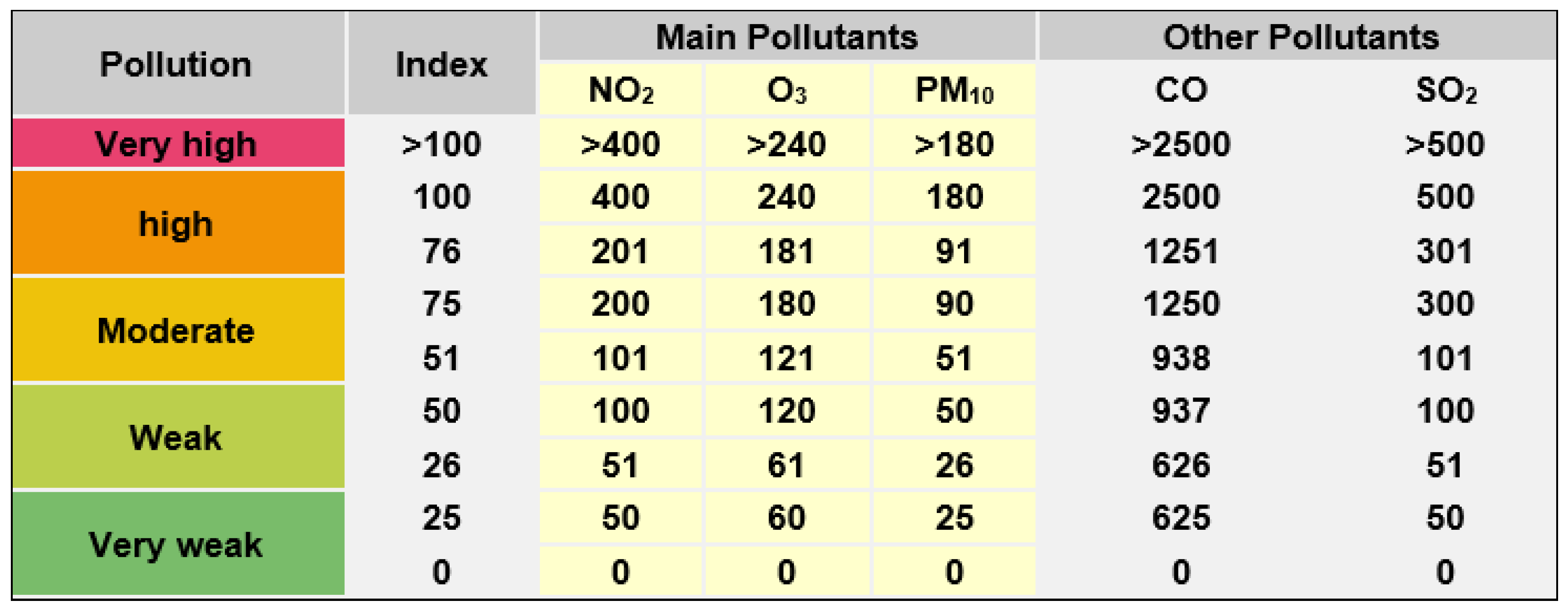
- Particulate matter (PM) describes inhalable particles with diameters of 10 micrometres and smaller;
- Nitrogen dioxide (NO) is a highly reactive gas that primarily gets into the air from the burning of fuel;
- Ozone (O) is a highly reactive gas composed of three oxygen atoms. Ground-level ozone, which we can breathe, is formed primarily from photochemical reactions between two major classes of air pollutants: volatile organic compounds (VOC) and nitrogen oxides (NO);
- Carbon monoxide (CO), which is a colourless, odourless gas that can be harmful when inhaled in large amounts. CO is released when something is burned. The greatest sources of CO in outdoor air are cars, trucks and other vehicles or machinery that burn fossil fuels;
- Sulfur dioxide (SO), which results from the burning of either sulfur or materials containing sulfur. SO emissions lead to the formation of other sulfur oxides, which can react with other compounds in the atmosphere to form small particles. Short-term exposures to SO can lead to respiratory problems.
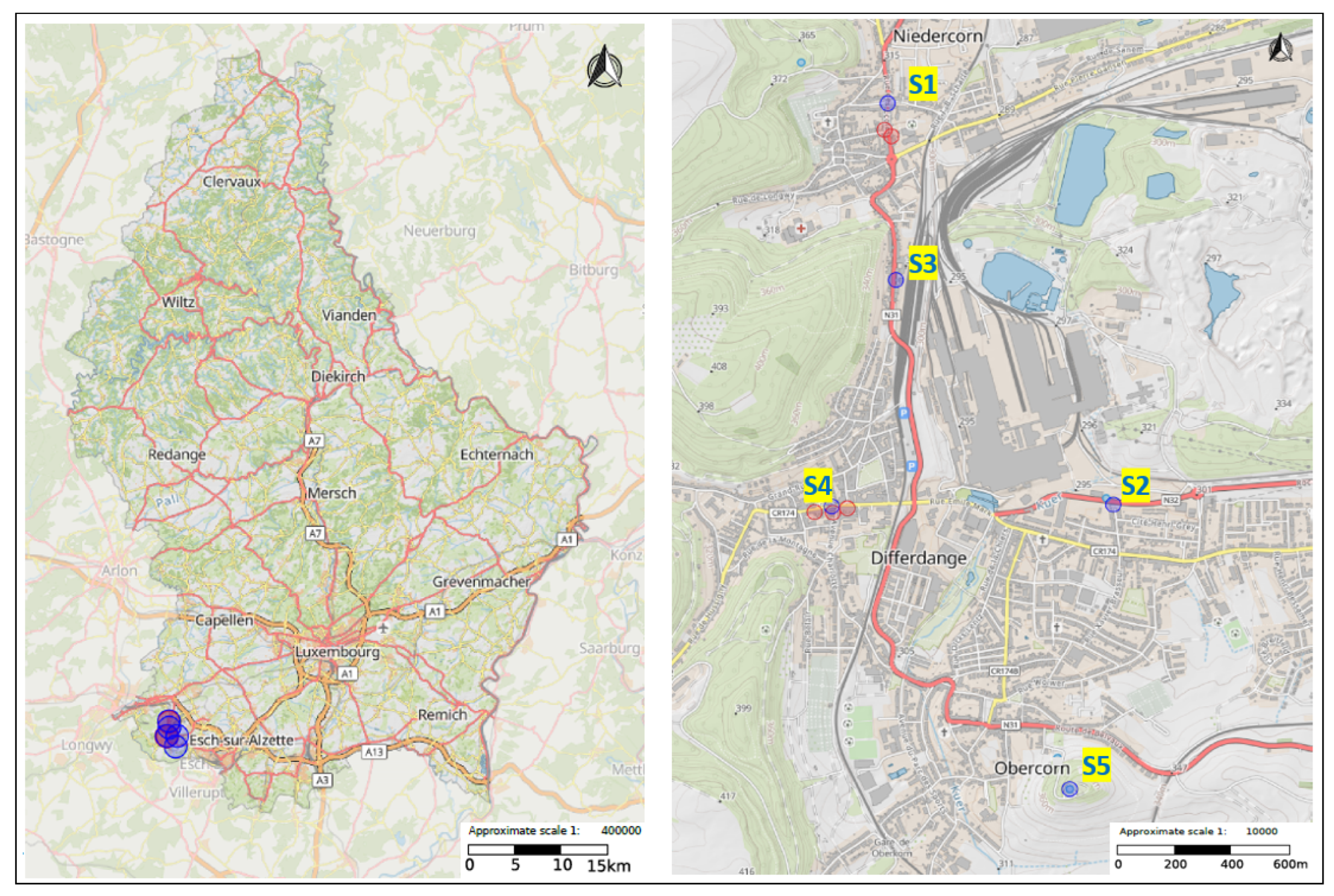
2. Data Description
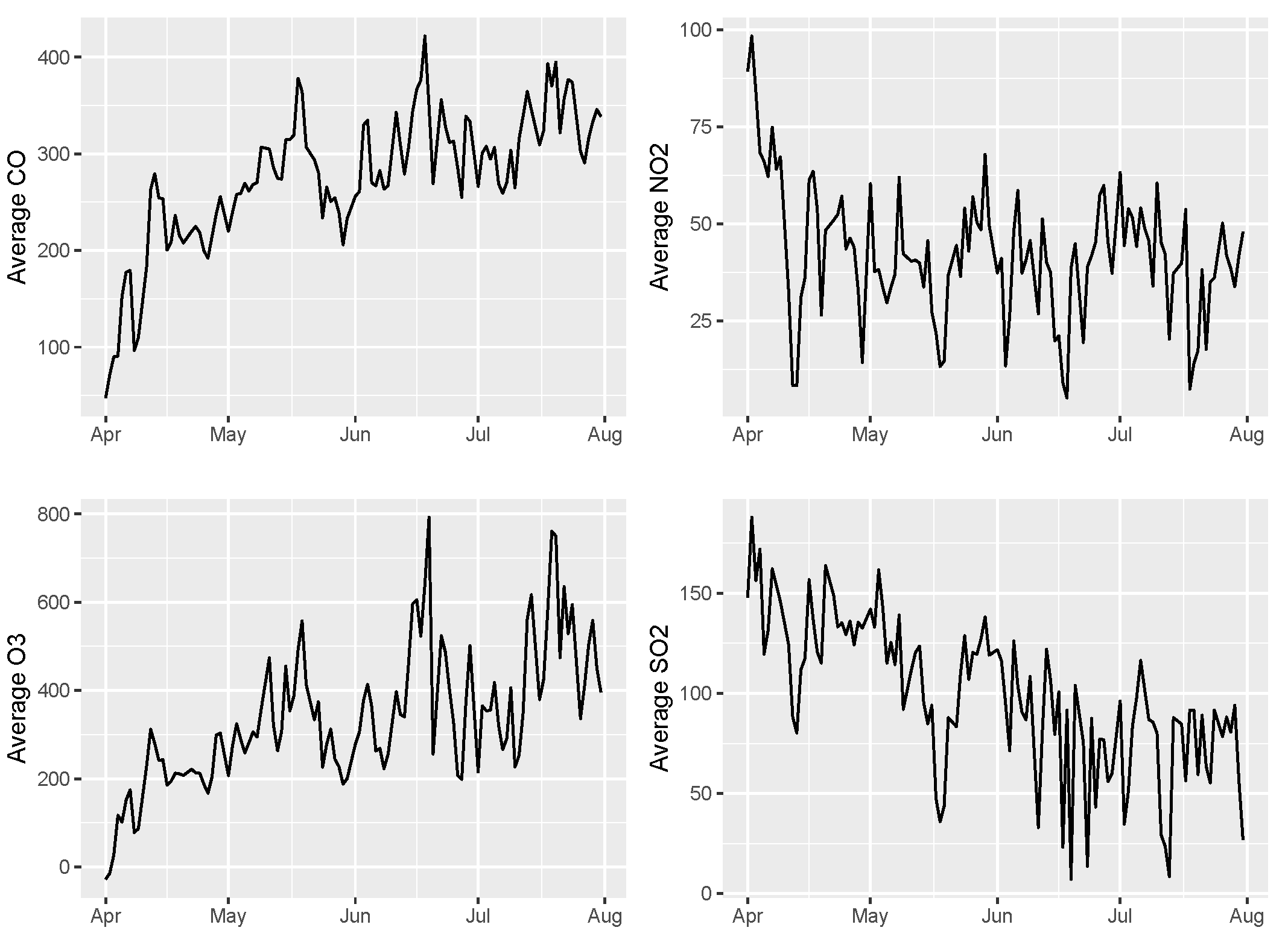
2.1. Air Quality Data
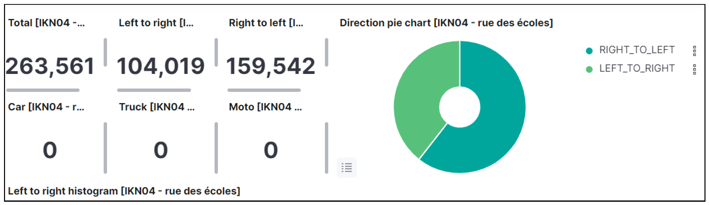
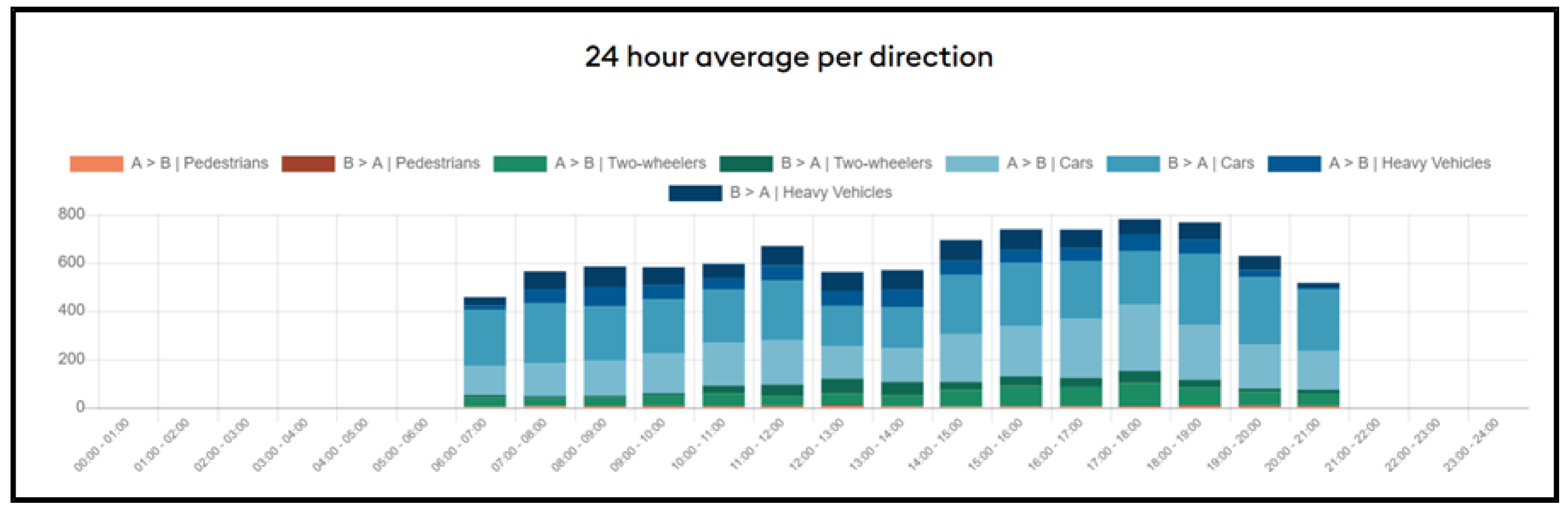
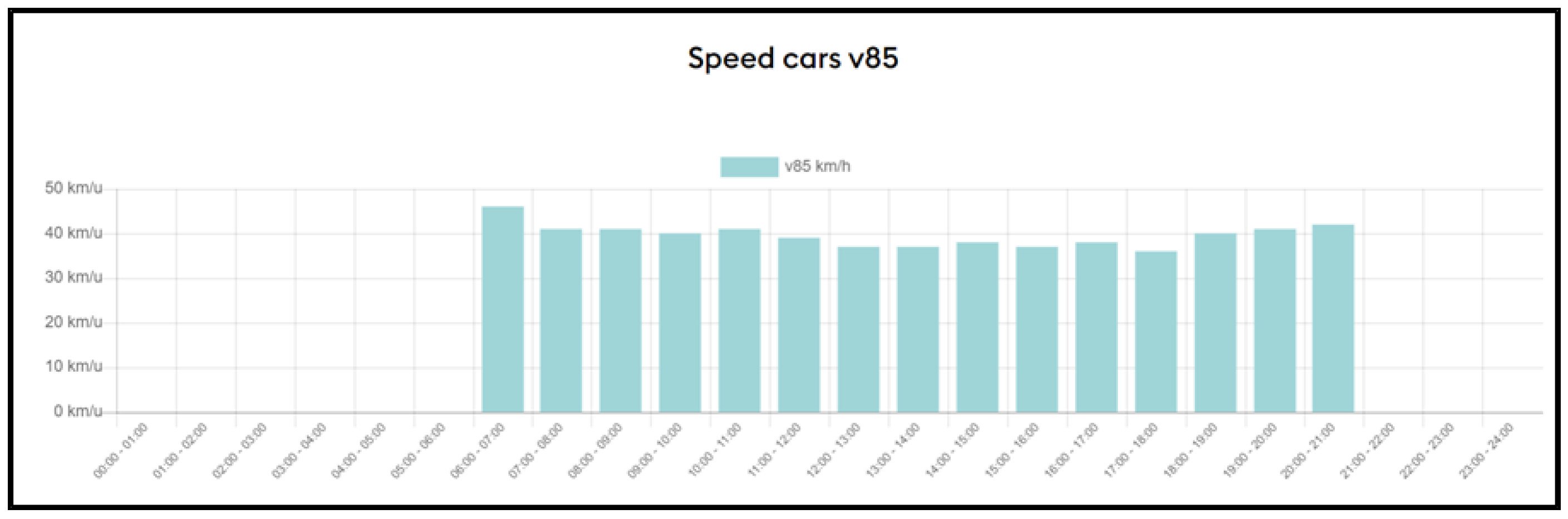
2.2. Traffic Data
2.2.1. Acoustic Sensors
2.2.2. Object Detection Sensors
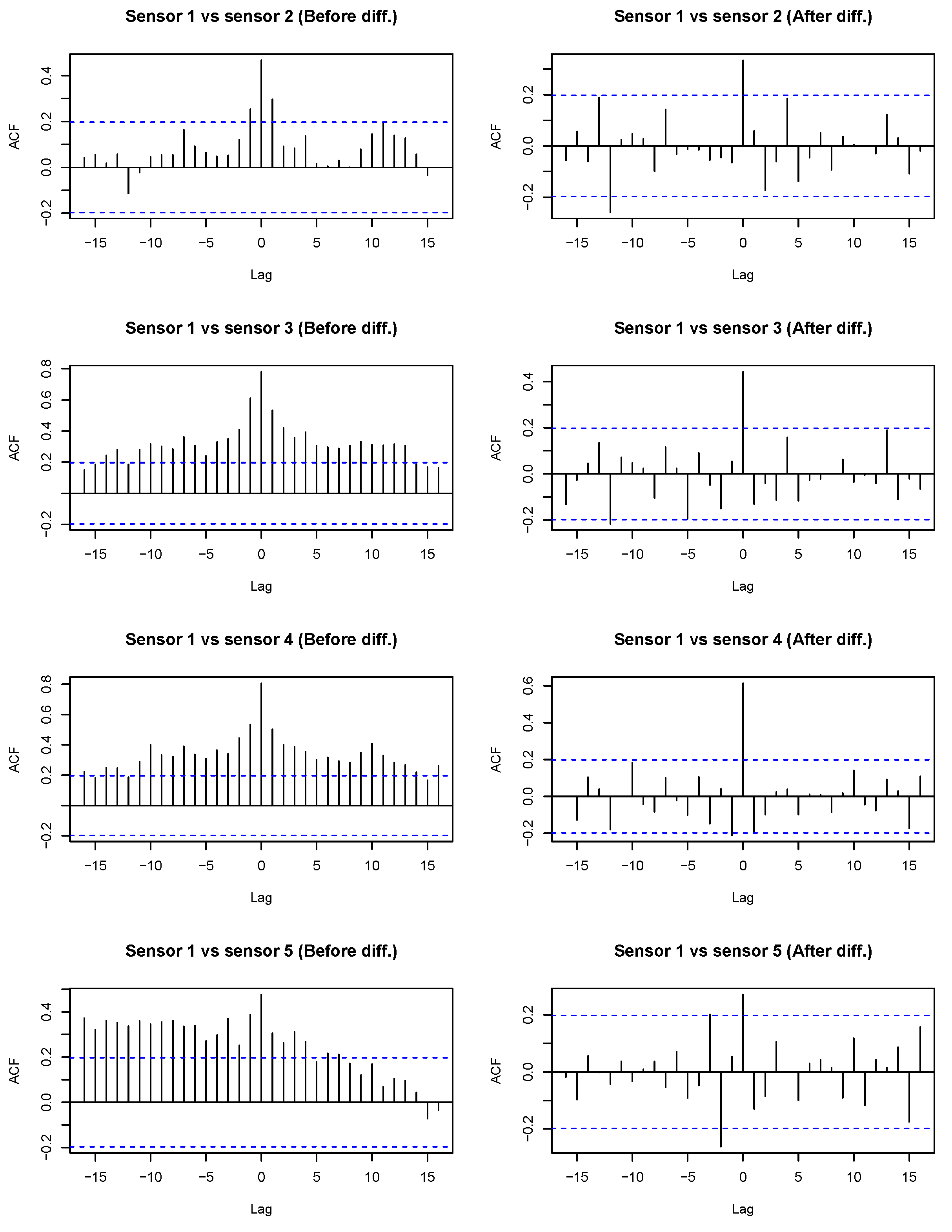
2.3. Differentiation of the Collected Data
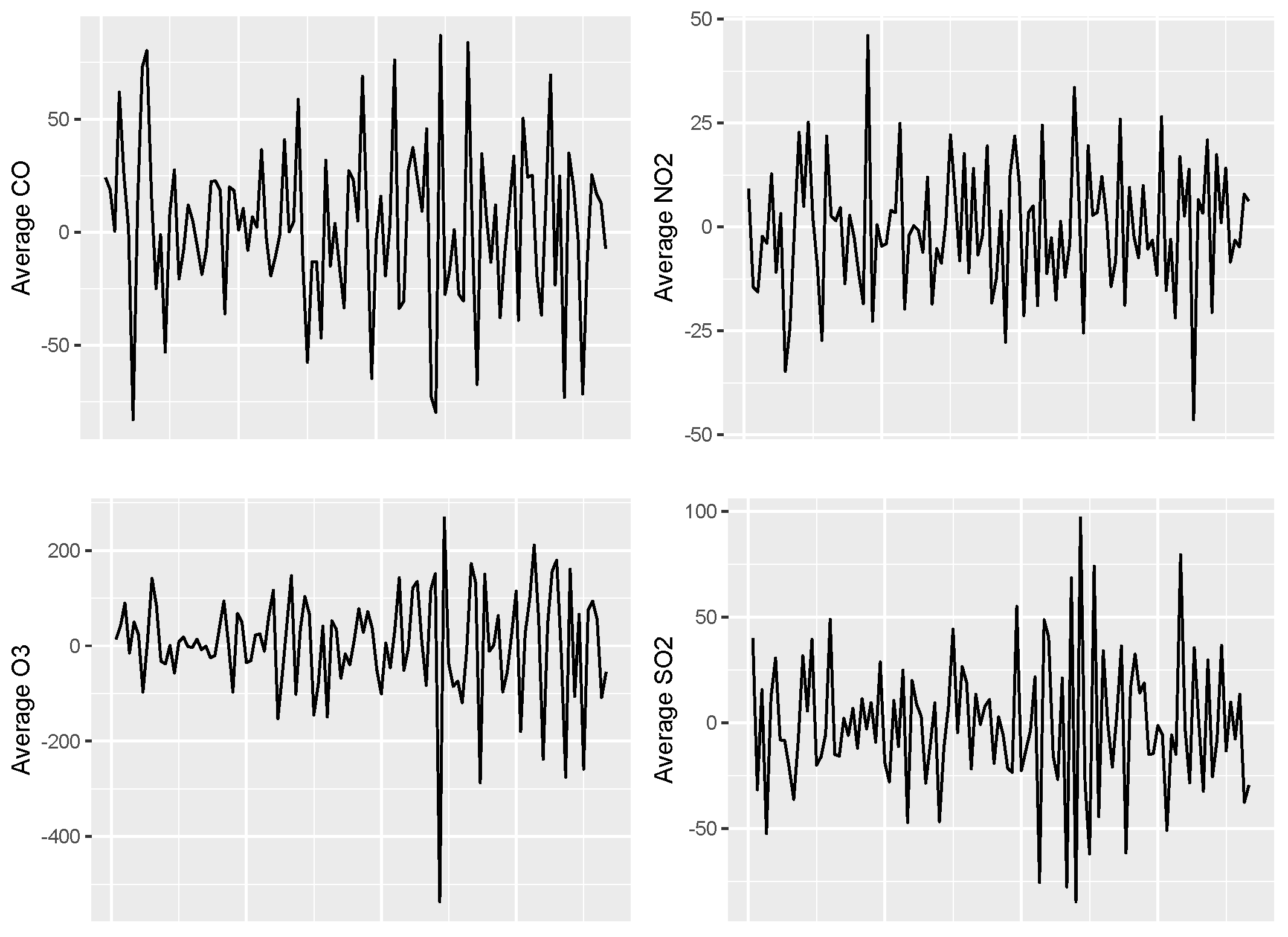
3. Time-Series Clustering
3.1. Description of the Method
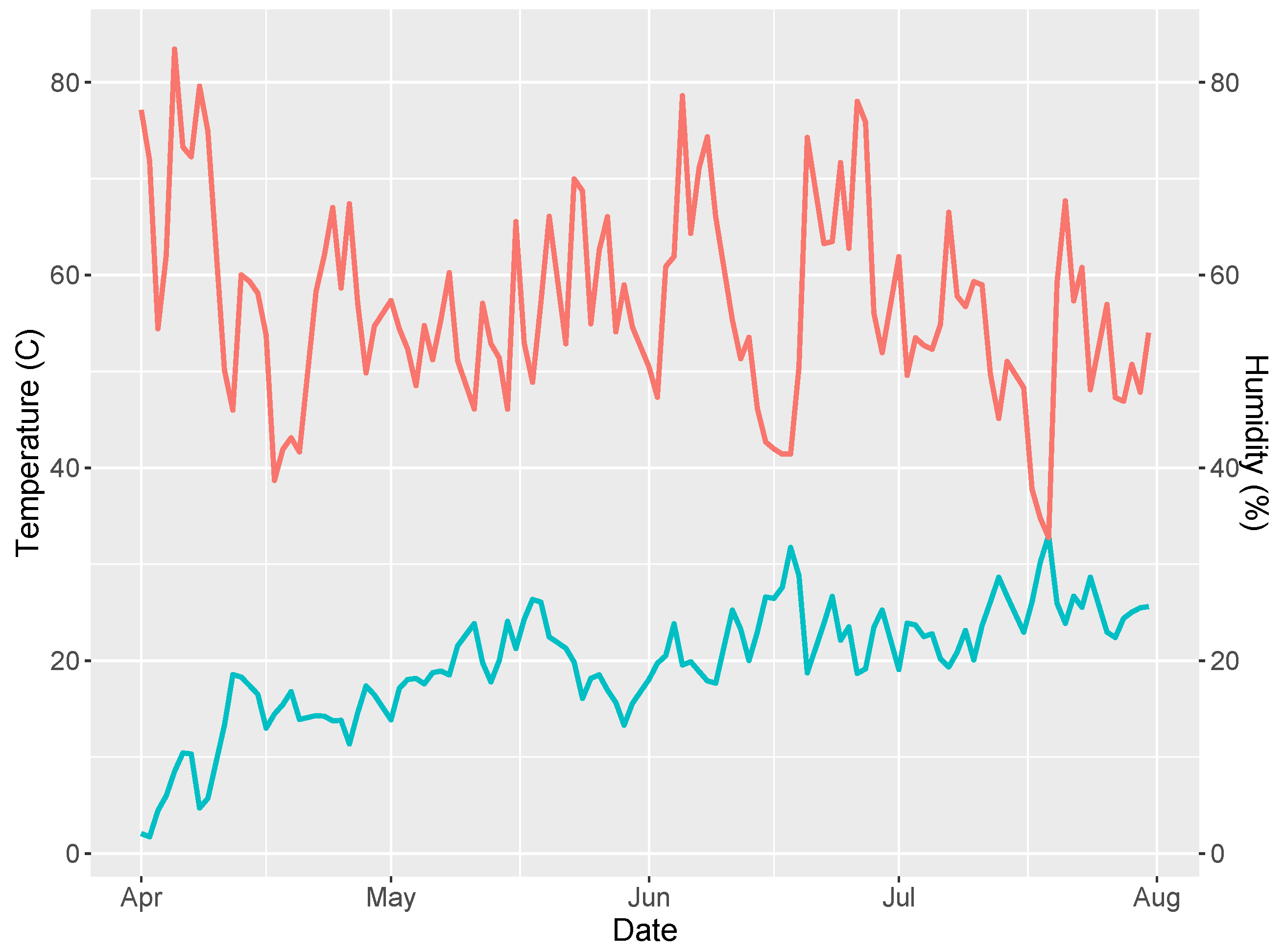
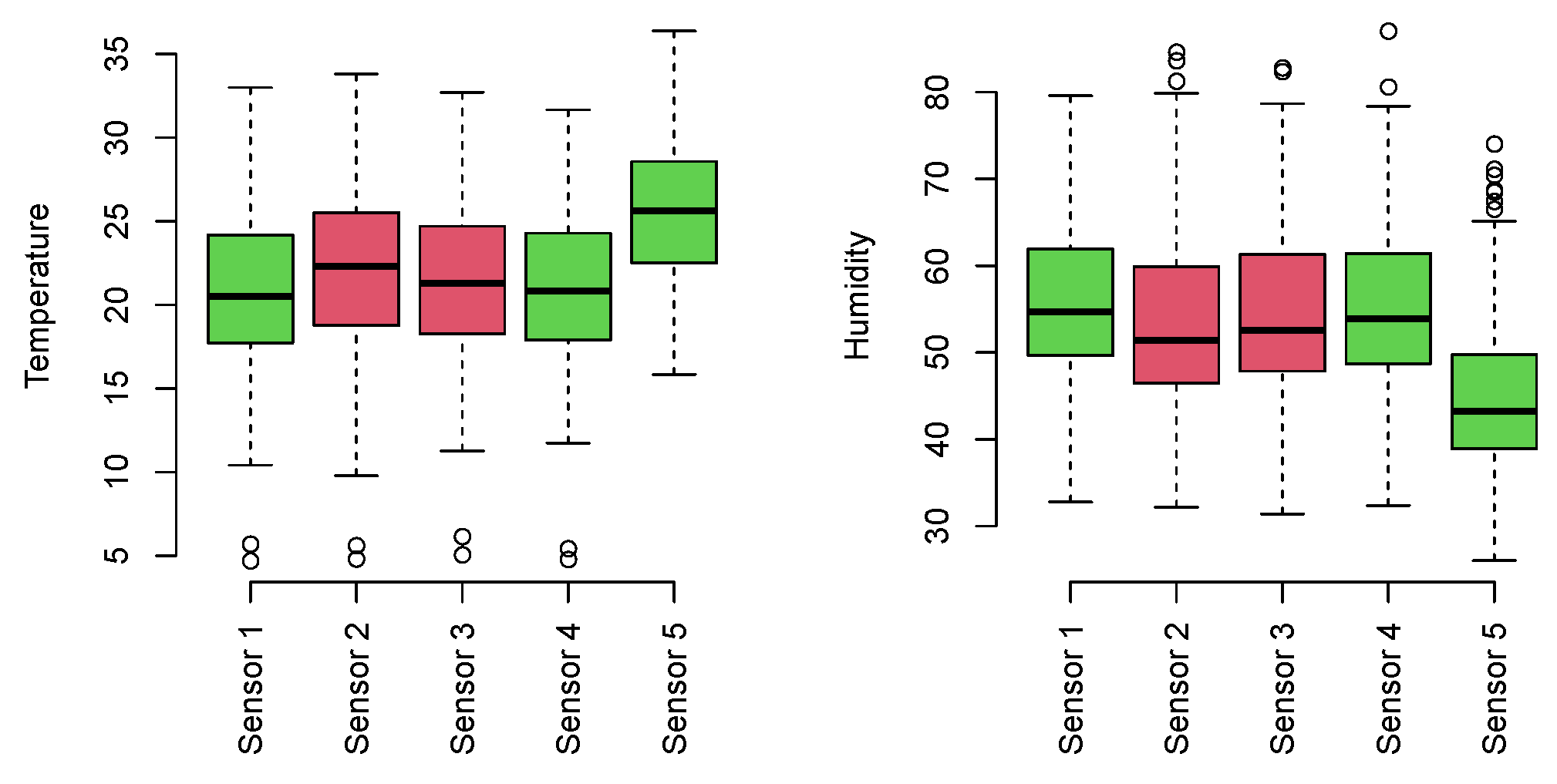
3.2. Temporal Behavior of Each Pollutant with respect to the Temperature and the Humidity
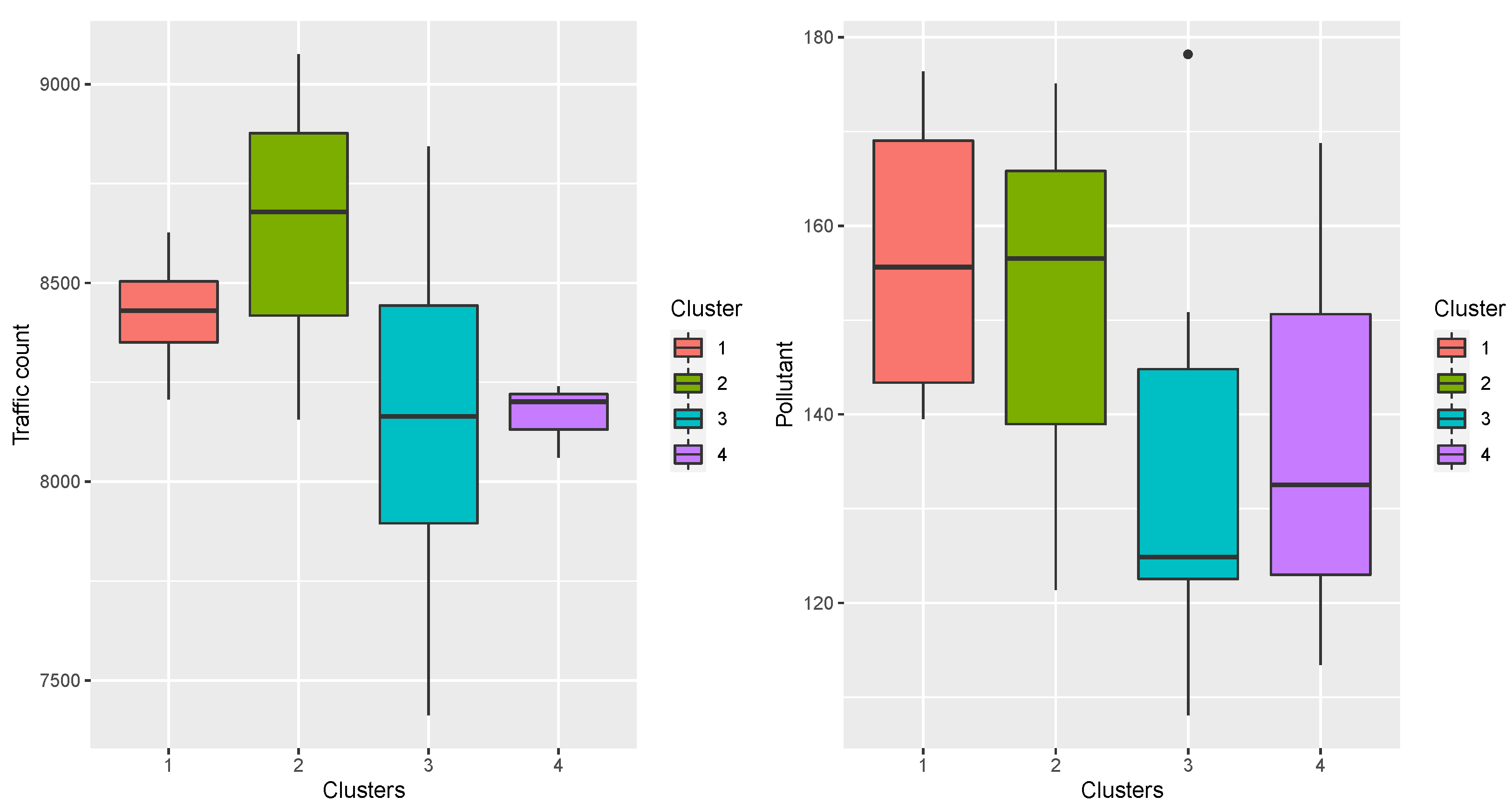
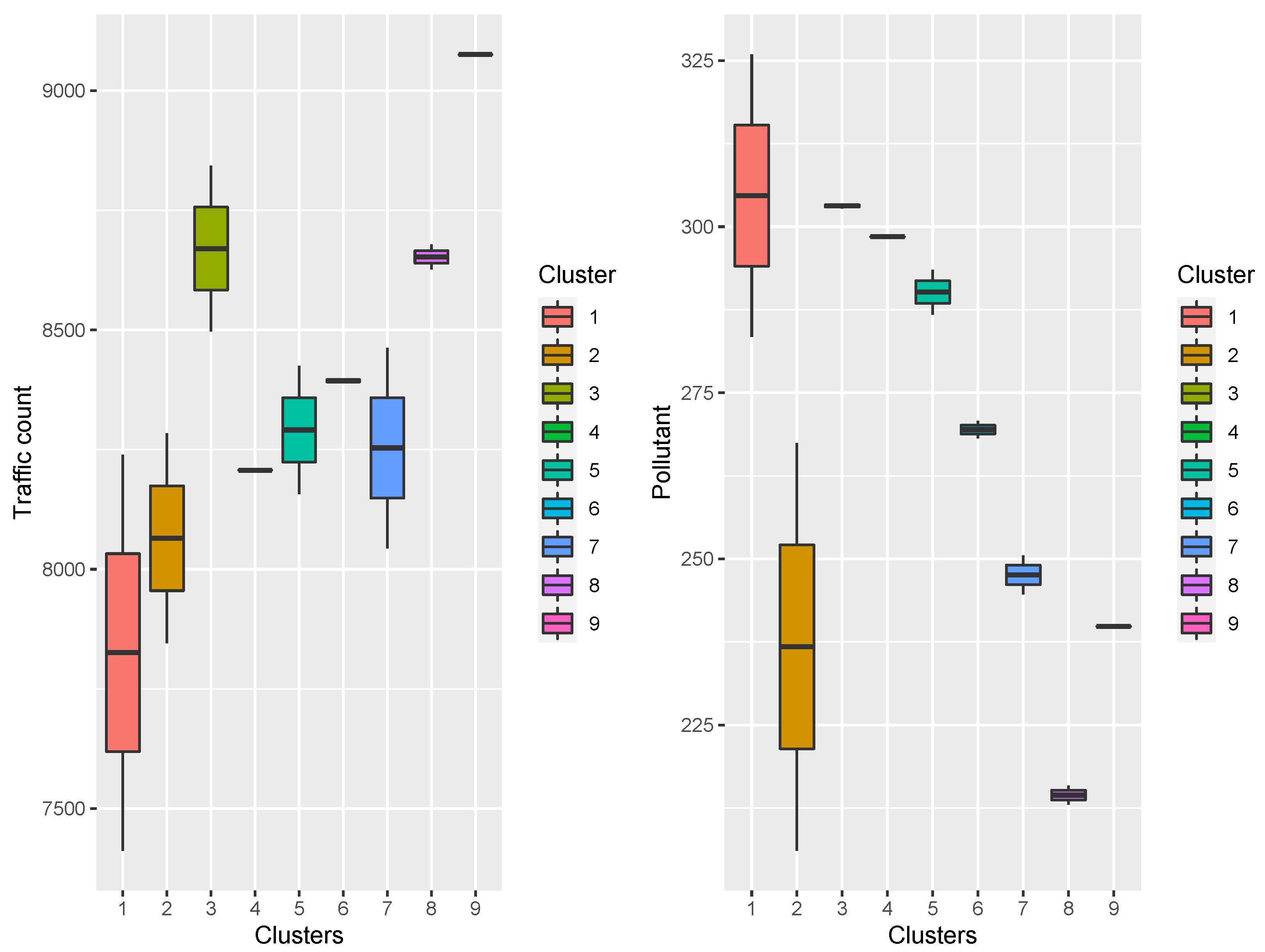
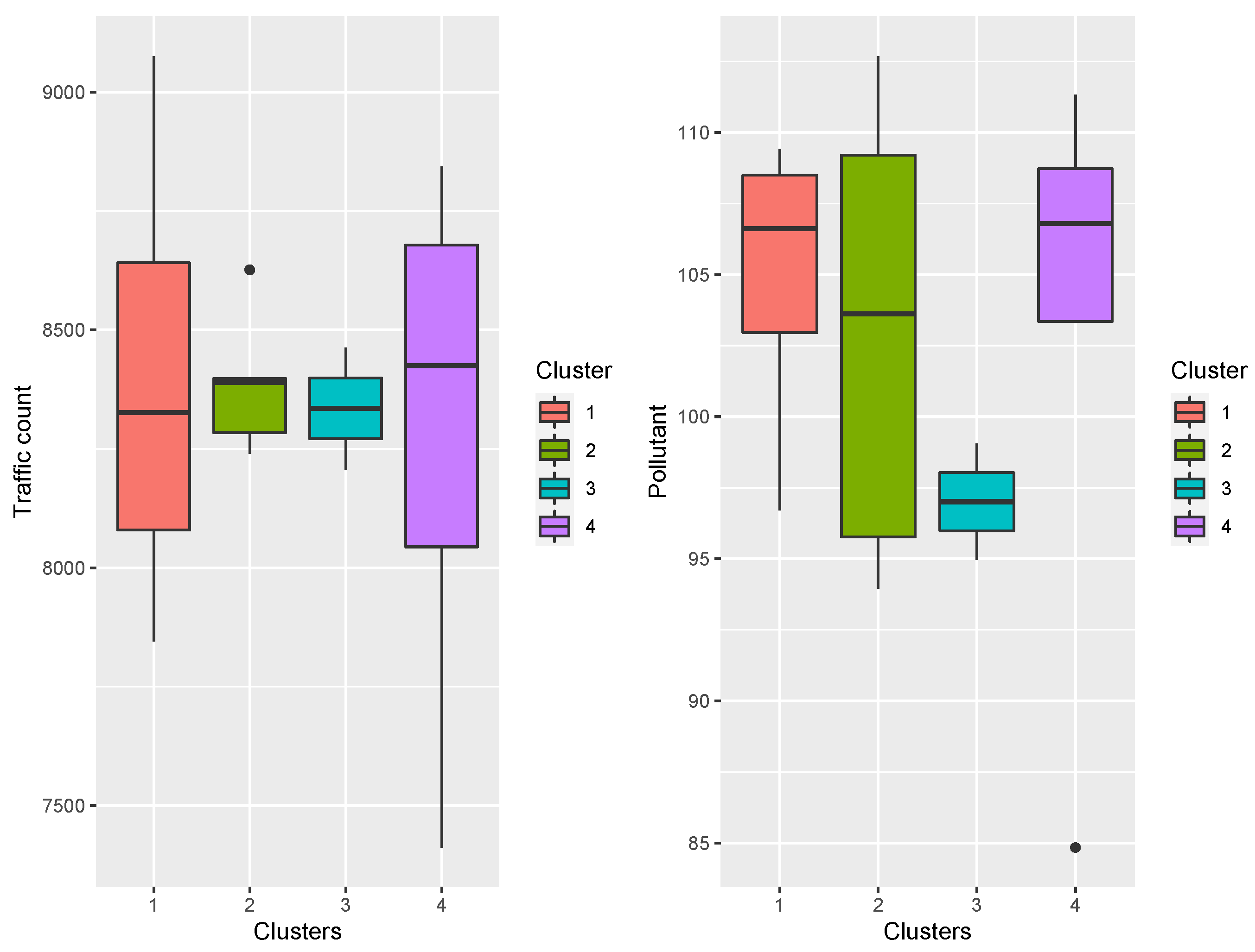
3.3. Temporal Behavior of Each Pollutant with Respect to the Traffic
4. Conclusions and Perspectives for Future Works
Author Contributions
Funding
Acknowledgments
Conflicts of Interest
References
- European Environment Agency. Greenhouse Gas Emissions from Transport in Europe; European Environment Agency: Copenhagen, Denmark, 2021.
- European Environment Agency. Air Quality in Europe 2021; European Environment Agency: Copenhagen, Denmark, 2021; Volume 15/2021. [CrossRef]
- European Environment Agency. Directive 2008/50/CE du Parlement Europeen et du Conseil du 21 mai 2008 Concernant la Qualité de l’air Ambiant et un Air pur Pour l’Europe. 2008. Available online: http://data.europa.eu/eli/dir/2008/50/oj (accessed on 12 January 2023).
- World Health Organization. WHO Global Air Quality Guidelines: Particulate Matter (PM2.5 and PM10), Ozone, Nitrogen Dioxide, Sulfur Dioxide and Carbon Monoxide; World Health Organization: Geneva, Switzerland, 2021; p. 273. [Google Scholar]
- Aggoune-Mtalaa, W.; Aggoune, R. An optimization algorithm to schedule care for the elderly at home. Int. J. Inf. Sci. Intell. Syst. 2014, 3, 41–50. [Google Scholar]
- Djenouri, Y.; Habbas, Z.; Aggoune-Mtalaa, W. Bees swarm optimization metaheuristic guided by decomposition for solving MAX-SAT. In Proceedings of the ICAART 2016–Proceedings of the 8th International Conference on Agents and Artificial Intelligence, Rome, Italy, 24–26 February 2016; Volume 2, pp. 472–479. [Google Scholar]
- Nasri, S.; Bouziri, H.; Aggoune-Mtalaa, W. Dynamic on Demand Responsive Transport with Time-Dependent Customer Load. In Proceedings of the Innovations in Smart Cities Applications Volume 4: Lecture Notes in Networks and Systems; Springer International Publishing: Cham, Switzerland, 2021; pp. 395–409. [Google Scholar]
- Nasri, S.; Bouziri, H.; Aggoune-Mtalaa, W. An Evolutionary Descent Algorithm for Customer-Oriented Mobility-On-Demand Problems. Sustainability 2022, 14, 3020. [Google Scholar] [CrossRef]
- Rezgui, D.; Siala, J.C.; Aggoune-Mtalaa, W.; Bouziri, H. Towards smart urban freight distribution using fleets of modular electric vehicles. In Innovations in Smart Cities and Applications: Proceedings of the 2nd Mediterranean Symposium on Smart City Applications 2; Lecture Notes in Networks and Systems; Springer: Berlin/Heidelberg, Germany, 2018; Volume 37. [Google Scholar]
- Rezgui, D.; Bouziri, H.; Aggoune-Mtalaa, W.; Siala, J.C. A Hybrid Evolutionary Algorithm for Smart Freight Delivery with Electric Modular Vehicles. In Proceedings of the 2018 IEEE/ACS 15th International Conference on Computer Systems and Applications (AICCSA), Aqaba, Jordan, 28 October–1 November 2018; pp. 1–8. [Google Scholar]
- Rezgui, D.; Bouziri, H.; Aggoune-Mtalaa, W.; Siala, J.C. An Evolutionary Variable Neighborhood Descent for Addressing an Electric VRP Variant. In Variable Neighborhood Search: 6th International Conference, ICVNS 2018, Sithonia, Greece, 4–7 October 2018, Revised Selected Papers 6; Lecture Notes in Computer Science; Springer: Berlin/Heidelberg, Germany, 2019; Volume 11328, pp. 216–231. [Google Scholar]
- Faye, S.; Melakessou, F.; Mtalaa, W.; Gautier, P.; AlNaffakh, N.; Khadraoui, D. SWAM: A Novel Smart Waste Management Approach for Businesses using IoT. In Proceedings of the TESCA’19: Proceedings of the 1st ACM International Workshop on Technology Enablers and Innovative Applications for Smart Cities and Communities, New York, NY, USA, 13–14 November 2019; p. 38. [CrossRef]
- Mohapatra, H.; Mohanta, B.K.; Nikoo, M.R.; Daneshmand, M.; Gandomi, A.H. MCDM Based Routing for IoT Enabled Smart Water Distribution Network. IEEE Internet Things J. 2023, 10, 4271–4280. [Google Scholar] [CrossRef]
- Fernandez-Prieto, J.A.; Canada-Bago, J.; Birkel, U. A Fuzzy Rule-Based System to Infer Subjective Noise Annoyance Using an Experimental Wireless Acoustic Sensor Network. Smart Cities 2022, 5, 1574–1589. [Google Scholar] [CrossRef]
- Mohapatra, H. Socio-technical Challenges in the Implementation of Smart City. In Proceedings of the 2021 International Conference on Innovation and Intelligence for Informatics, Computing, and Technologies (3ICT), Zallaq, Bahrain, 29–30 September 2021; pp. 57–62. [Google Scholar] [CrossRef]
- Jonek-Kowalska, I. Assessing the Effectiveness of Air Quality Improvements in Polish Cities Aspiring to be Sustainably Smart. Smart Cities 2023, 6, 510–530. [Google Scholar] [CrossRef]
- Karagulian, F.; Barbiere, M.; Kotsev, A.; Spinelle, L.; Gerboles, M.; Lagler, F.; Redon, N.; Crunaire, S.; Borowiak, A. Review of the Performance of Low-Cost Sensors for Air Quality Monitoring. Atmosphere 2019, 10, 506. [Google Scholar] [CrossRef] [Green Version]
- Ameer, S.; Shah, M.A.; Khan, A.; Song, H.; Maple, C.; Islam, S.U.; Asghar, M.N. Comparative Analysis of Machine Learning Techniques for Predicting Air Quality in Smart Cities. IEEE Access 2019, 7, 128325–128338. [Google Scholar] [CrossRef]
- Kumar, R.; Peuch, V.H.; Crawford, J.H.; Brasseur, G. Five Steps to Improve Air-Quality Forecasts. 2018. Available online: https://www.nature.com/articles/d41586-018-06150-5 (accessed on 12 January 2023).
- Lin, C.; Huang, R.J.; Ceburnis, D.; Buckley, P.; Preissler, J.; Wenger, J.; Rinaldi, M.; Facchini, M.C.; O’Dowd, C.; Ovadnevaite, J. Extreme air pollution from residential solid fuel burning. Nat. Sustain. 2018, 1, 512. [Google Scholar] [CrossRef]
- Belis, C.; Karagulian, F.; Larsen, B.R.; Hopke, P. Critical review and meta-analysis of ambient particulate matter source apportionment using receptor models in Europe. Atmos. Environ. 2013, 69, 94–108. [Google Scholar] [CrossRef]
- Yatkin, S.; Bayram, A. Elemental composition and sources of particulate matter in the ambient air of a Metropolitan City. Atmos. Res. 2007, 85, 126–139. [Google Scholar] [CrossRef]
- Salcedo, R.; Ferraz, M.A.; Alves, C.; Martins, F. Time-series analysis of air pollution data. Atmos. Environ. 1999, 33, 2361–2372. [Google Scholar] [CrossRef]
- Broday, D.M. Studying the time scale dependence of environmental variables predictability using fractal analysis. Environ. Sci. & Technol. 2010, 44, 4629–4634. [Google Scholar]
- Meraz, M.; Rodriguez, E.; Femat, R.; Echeverria, J.; Alvarez-Ramirez, J. Statistical persistence of air pollutants (O3, SO2, NO2 and PM10) in Mexico City. Phys. A Stat. Mech. Its Appl. 2015, 427, 202–217. [Google Scholar] [CrossRef]
- Chen, Z.; Barros, C.P.; Gil-Alana, L.A. The persistence of air pollution in four mega-cities of China. Habitat Int. 2016, 56, 103–108. [Google Scholar] [CrossRef] [Green Version]
- Meraz, M.; Alvarez-Ramirez, J.; Echeverria, J. Asymmetric correlations in the ozone concentration dynamics of the Mexico City Metropolitan Area. Phys. A Stat. Mech. Its Appl. 2017, 471, 377–386. [Google Scholar] [CrossRef]
- Telesca, L.; Caggiano, R.; Lapenna, V.; Lovallo, M.; Trippetta, S.; Macchiato, M. The Fisher information measure and Shannon entropy for particulate matter measurements. Phys. A Stat. Mech. Its Appl. 2008, 387, 4387–4392. [Google Scholar] [CrossRef]
- Telesca, L.; Caggiano, R.; Lapenna, V.; Lovallo, M.; Trippetta, S.; Macchiato, M. Analysis of dynamics in Cd, Fe, and Pb in particulate matter by using the Fisher–Shannon method. Water Air Soil Pollut. 2009, 201, 33–41. [Google Scholar] [CrossRef]
- Telesca, L.; Lovallo, M. Complexity analysis in particulate matter measurements. Comput. Ecol. Softw. 2011, 1, 146. [Google Scholar]
- Amato, F.; Laib, M.; Guignard, F.; Kanevski, M. Analysis of air pollution time series using complexity-invariant distance and information measures. Phys. A Stat. Mech. Its Appl. 2020, 547, 124391. [Google Scholar] [CrossRef]
- R. Lamm, E.C. Rural Roads Speed Inconsistencies Design Methods. In Research Report for the State University of New York; Research Foundation: Albany, NY, USA, 1987; Volume Parts I and II. [Google Scholar]
- Agency Environment Agency. Current Speed Limit Policies-Mobility and Transport-European Commission. 2008. Available online: https://road-safety.transport.ec.europa.eu/eu-road-safety-policy/priorities/safe-road-use/safe-speed/archive/currentspeed-limit-policies_en (accessed on 12 January 2023).
- Hastie, T.; Tibshirani, R.; Friedman, J. Unsupervised Learning. In The Elements of Statistical Learning: Data Mining, Inference, and Prediction; Springer New York: New York, NY, USA, 2009; pp. 485–585. [Google Scholar]
- Montero, P.; Vilar, J.A. TSclust: An R Package for Time Series Clustering. J. Stat. Softw. 2014, 62, 1–43. [Google Scholar] [CrossRef] [Green Version]
- Warren Liao, T. Clustering of time series data—A survey. Pattern Recognit. 2005, 38, 1857–1874. [Google Scholar] [CrossRef]
- Partitioning Around Medoids (Program PAM). In Finding Groups in Data; John Wiley & Sons, Ltd.: Hoboken, NJ, USA, 1990; Chapter 2; pp. 68–125. [CrossRef]
- Jain, A.K. Data clustering: 50 years beyond K-means. Pattern Recognit. Lett. 2010, 31, 651–666. [Google Scholar] [CrossRef]
- Golay, X.; Kollias, S.; Stoll, G.; Meier, D.; Valavanis, A.; Boesiger, P. A new correlation-based fuzzy logic clustering algorithm for FMRI. Magn. Reson. Med. 1998, 40, 249–260. [Google Scholar] [CrossRef] [PubMed]


| Air quality | Sources | 5 |
| Instances | 320 | |
| Weather | Sources | 5 |
| Instances | 160 | |
| Traffic count | Sources | 13 |
| Instances | 208 |
Disclaimer/Publisher’s Note: The statements, opinions and data contained in all publications are solely those of the individual author(s) and contributor(s) and not of MDPI and/or the editor(s). MDPI and/or the editor(s) disclaim responsibility for any injury to people or property resulting from any ideas, methods, instructions or products referred to in the content. |
© 2023 by the authors. Licensee MDPI, Basel, Switzerland. This article is an open access article distributed under the terms and conditions of the Creative Commons Attribution (CC BY) license (https://creativecommons.org/licenses/by/4.0/).
Share and Cite
Aggoune-Mtalaa, W.; Laib, M. Analyzing Air Pollution and Traffic Data in Urban Areas in Luxembourg. Smart Cities 2023, 6, 929-943. https://doi.org/10.3390/smartcities6020045
Aggoune-Mtalaa W, Laib M. Analyzing Air Pollution and Traffic Data in Urban Areas in Luxembourg. Smart Cities. 2023; 6(2):929-943. https://doi.org/10.3390/smartcities6020045
Chicago/Turabian StyleAggoune-Mtalaa, Wassila, and Mohamed Laib. 2023. "Analyzing Air Pollution and Traffic Data in Urban Areas in Luxembourg" Smart Cities 6, no. 2: 929-943. https://doi.org/10.3390/smartcities6020045