A Complete Pipeline for Heart Rate Extraction from Infant ECGs

Abstract

Infant electrocardiograms (ECGs) and heart rates (HRs) are very useful biosignals for psychological research and clinical work, but can be hard to analyse properly, particularly longform (≥5 min) recordings taken in naturalistic environments. Infant HRs are typically much faster than adult HRs, and so some of the underlying frequency assumptions made about adult ECGs may not hold for infants. However, the bulk of publicly available ECG approaches focus on adult data. Here, existing open source ECG approaches are tested on infant datasets. The best-performing open source method is then modified to maximise its performance on infant data (e.g., including a 15 Hz high-pass filter, adding local peak correction). The HR signal is then subsequently analysed, developing an approach for cleaning data with separate sets of parameters for the analysis of cleaner and noisier HRs. A Signal Quality Index (SQI) for HR is also developed, providing insights into where a signal is recoverable and where it is not, allowing for more confidence in the analysis performed on naturalistic recordings. The tools developed and reported in this paper provide a base for the future analysis of infant ECGs and related biophysical characteristics. Of particular importance, the proposed solutions outlined here can be efficiently applied to real-world, large datasets.

1. Introduction

Although heart rate (HR) has been used for studying infant cognitive and emotional developments for several decades, there are currently few evaluations of complete open access pipelines, especially focussing on infant data recorded in naturalistic environments while infants are free to move. Measures of the cardiovascular system provide a clear window into the activity of the autonomic nervous system (ANS), reflecting innervations from both the sympathetic and parasympathetic branches [1]. Variations in heart period and heart rate variabilities have been linked to important cognitive functions, such as attention, memory, and information processing, as well as changes in arousal and regulatory abilities [2,3,4,5]. ANS activity measurement has been fruitful for understanding both typical and atypical developments, with atypical ANSs shown in manifestations of autism spectrum disorders [6,7,8], attention deficit and hyperactivity disorders [9], conduct disorders [10], as well as the emergence of other neuropsychiatric conditions [11]. Cardiovascular measures are particularly useful for the study of cognitive and emotional developments beginning with the first days of life since both the cardiovascular and autonomic systems are well developed at birth [12], and electrocardiography (ECG) recordings can be obtained in a non-invasive fashion. In the context of infants’ limited behavioural repertoire, reduced motor development, and lack of verbal communication abilities, non-invasive methods that can provide insights into cognitive and emotion functions are essential for understanding how these develop within the critical first 1000 days of life. With advances in wearable sensing technology, ECG recordings can be more easily obtained outside the laboratory as well, allowing dense recordings over hours and days [13,14]. The main motivation of this paper is to develop an innovative novel framework for studying this development in the natural environment, allowing researchers to understand the complexity of factors that can contribute to typical and atypical outcomes [15].

Children, and in particular infants, have a much higher HR than adults [16], and so algorithms tailored to process adult heart signals might not be the optimal choice for processing the signals recorded from an infant heart [17,18]. In addition to the higher heart rate, there are many other factors (e.g., differing ECG complex shapes that occur) that should be considered when using ECGs from infants and children [19]. Free movement during typical activities and lengthy recordings can produce more motion-induced noise, such as baseline wander and motion artefacts [20,21], which can be particularly problematic when cardiac activity is recorded for infants in naturalistic settings (e.g., their everyday home environment). This is in addition to other forms of ECG noise, such as power-line interference, and signal processing artefacts [22,23] that must be accounted for in ECG processing [24]. Recent early-development research has focussed on foetal heart rates and ECGs [25,26,27], rather than the specific issues surrounding infants. Building on and extending our previous work [13], the motivation of the current study is to propose a complete open source processing pipeline for longform infant ECG recordings (≥5 min) and validate them under a range of conditions (including naturalistic conditions) against open source state-of-the-art approaches. Compared to our previous work, we increase dataset sizes, include ECG data recordings from a range of devices recorded at a range of sampling rates, and present a more thorough validation of the different steps of the pipeline.

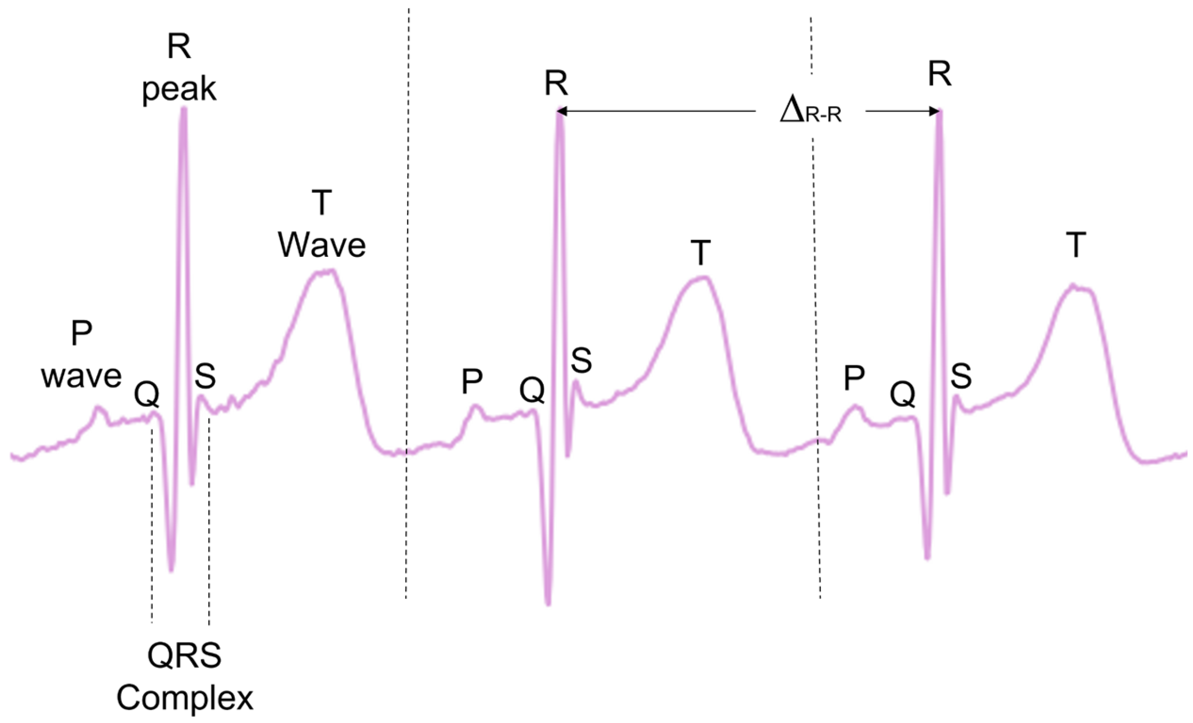
During typical functioning, the depolarisation of the heart ventricles produces a short and characteristic spike of electric signals, often referred to as the QRS complex, with the peak of the QRS complex referred to as the R-peak (Figure 1). When detected, the times between consecutive R-peaks (Δ_R-R) can be used to calculate the instantaneous HR in beats per minute (see Equation (1)). This provides a precise beat-by-beat HR measurement derived from the ECG.

HR = 60/(Δ_R-R)

(1)

There are many pre-established open source methods designed to preprocess ECG data and then extract the R-peaks [28,29,30,31,32,33,34,35,36]. While some comparative analyses have been previously carried out [23,28], no analysis exists evaluating the effectiveness of these methodologies on the ECGS of infants and young children. Many of these methods also investigate other ECG complexes, such as T-waves and P-waves, as well as the QRS complex as a whole (Figure 1). In the present paper, only the R-peak detection is analysed.

For the ECG preprocessing step, usually a decision must be made as to whether the signal is of sufficient quality for further processing and analysis. Noise can be reduced by frequency-filtering approaches, with low-pass filters (LPFs) for removing aspects such as white noise, high-pass filtering (HPF) used for aspects such as baseline drift, bandpass filtering (BPF) to remove low-frequency and high-frequency noises, and notch filtering for mains interference. Alternatively, other approaches, such as wavelets and empirical mode decomposition, have also been used [37,38,39].

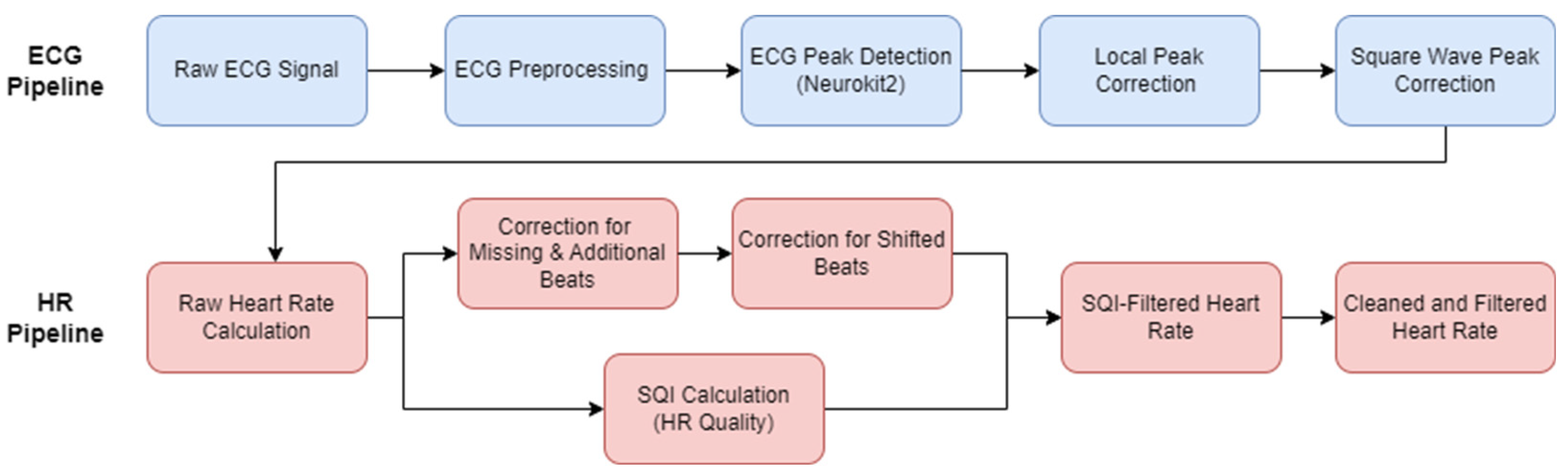
Typical ECG pipelines only encompass the preprocessing of the ECG signal and then the R-peak detection. Given the inherent noise level in infant and young children ECGs, and particularly ECG recordings in the natural environment, this paper aims to encapsulate the ECG to HR process as a complete open access pipeline, also accounting for any HR cleaning and HR signal quality measurements (Figure 2). First, pre-existing open access ECG pipelines from the literature were evaluated. The best-performing method was then chosen as the basis to develop our new open source pipeline for the infant ECGs and subsequent infant HR signals. A range of additional preprocessing options were evaluated, along with some ECG post-processing steps. The data and code that will be made available upon request is listed in Appendix A.

In brief, the key innovations in the proposed pipeline are as follows. The ECG preprocessing is improved by specifically tailoring the frequency filtering to infant ECGs. A local peak correction is added to allow for heavy filtering without affecting the underlying heart rate. A mathematically outlined approach is described for cleaning the HR signal in instances of minor mislabelling. A new HR signal quality index (SQI) is developed to help automatically reject areas of unrecoverable signals, which will help to account for the high levels of noise in infant ECG. Finally, a focus on computational efficiency was followed throughout to allow for the application to large amounts of data.

2. Materials and Results

In this section, existing ECG pipelines were applied to datasets containing infants and toddlers. Then, we proposed an adapted ECG pipeline (including two novel preprocessing approaches). Finally, we proposed a HR pipeline designed specifically to deal with longform and noisy recordings. All coding was done in Python (HeartPy-1.2.6, MatPlotLib-3.7.1 (purely for plotting), Neurokit2-0.2.3, Numpy-1.24.3, PyEMD-1.1.1, Scipy-1.10.1, Seaborn-0.12.2 (purely for plotting)) (Python Software Foundation, Wilmington, DE, USA).

2.1. Datasets

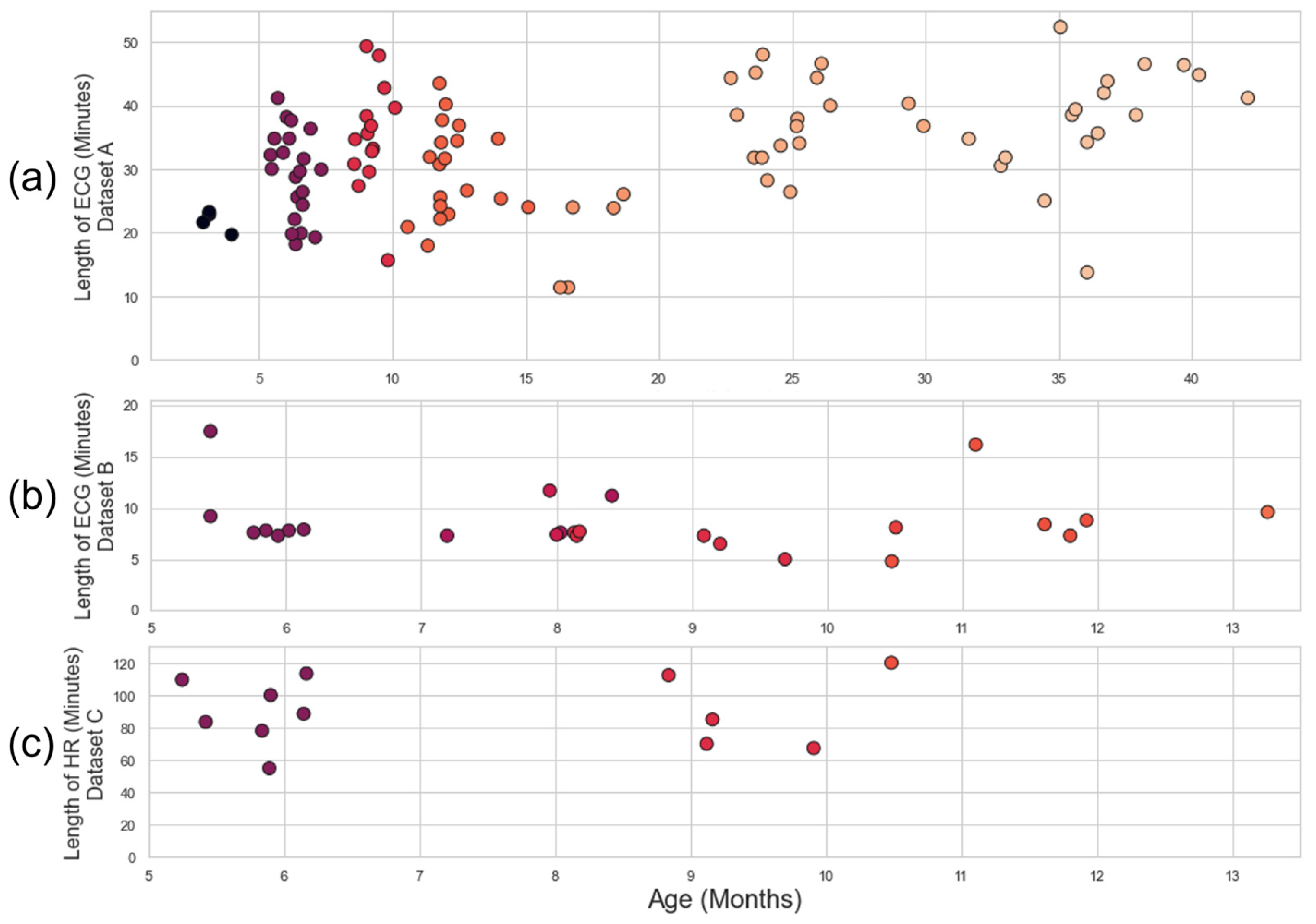
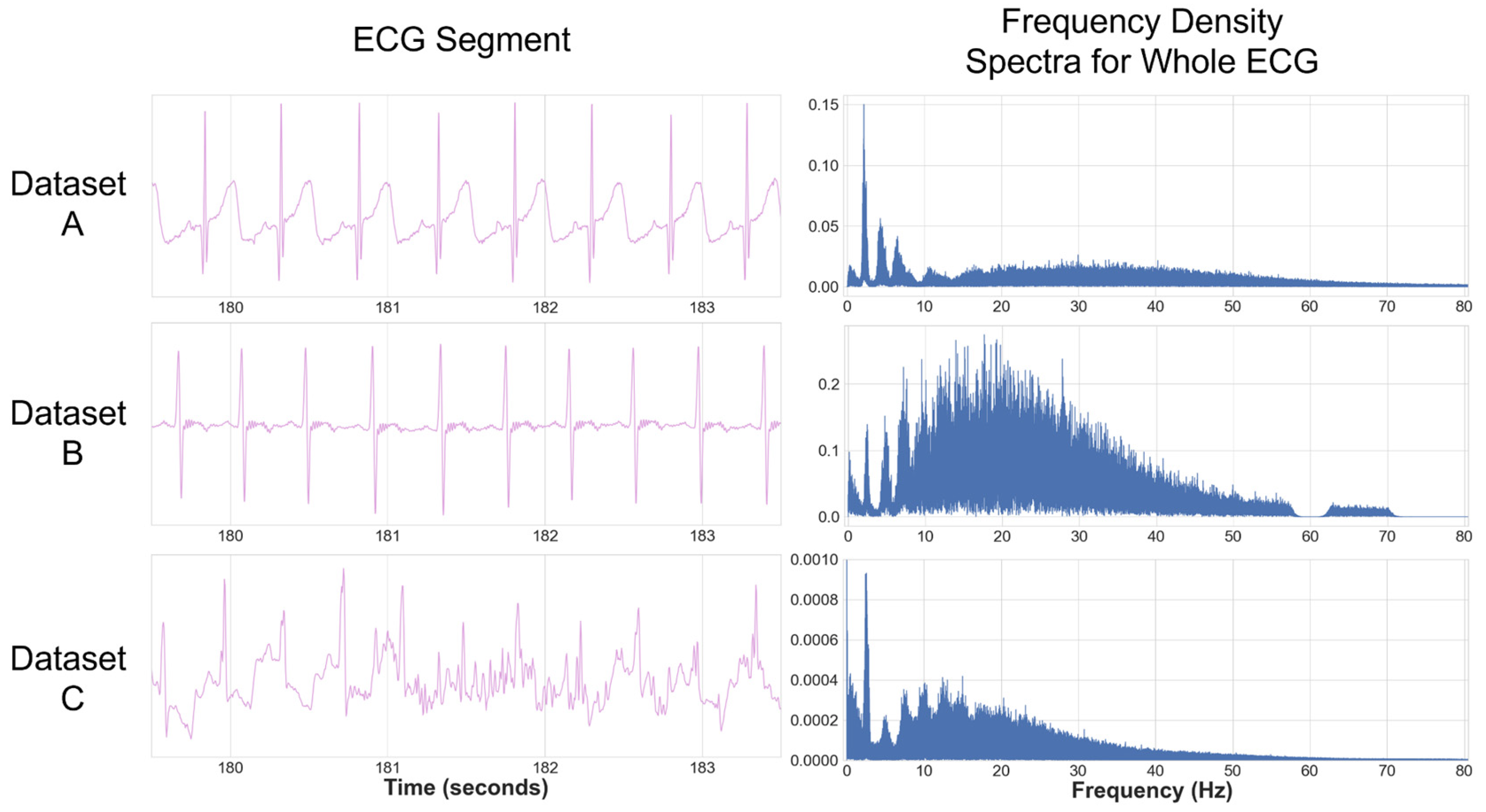
Three infant ECG datasets (

Table 1. The infant dataset information for the three datasets used in this paper. Age column shows the range and mean ± standard deviation. A breakdown of durations by age cohort provided given along with the overall total (shown in bold).

Dataset	Device	Sampling Rate (Hz)	Environment	Age (Months)	n	Total Duration	Mean Duration
A	Biosignalsplux (PLUX Biosignals, Lisbon, Portugal)	500	Research lab, Free play in infant play area	2.9–7.9 Mage = 5.8 ± 1.2	25	11 h, 41 min	28 min, 1 s
				8–10.9 Mage = 9.3 ± 0.6	15	8 h, 35 min	34 min, 20 s
				11–19.9 Mage = 13.4 ± 2.3	23	10 h, 41 min	27 min, 52 s
				20–42.3 Mage = 30.8 ± 6.2	34	21 h, 14 min	37 min, 45 s
				2.9–42.3 Mage = 16.9 ± 11.2	97	52 h, 20 min	32 min, 22 s
B	Geodesic EEG System (GES) 400 (Magstim EGI, USA)	1000	Research lab, Experimental testing (sitting on caregiver’s lap)	5.6–8.9 Mage = 7.1 ± 1.1	15	2 h, 13 min	8 min, 52 s
				9–13.0 Mage = 10.7 ± 1.3	10	1 h, 22 min	8 min, 12 s
				5.6–13.0 Mage = 8.5 ± 2.1	25	3 h, 34 min	8 min, 36 s
C	EgoActive sensor (University of York, UK)	250	Home environment, Free spontaneous behaviours	5.3–7.9 Mage = 5.8 ± 0.3	7	10 h, 27 min	89 min, 37 s
				8–10.4 Mage = 9.5 ± 0.7	5	7 h, 34 min	90 min, 51 s
				5.3–10.4 Mage = 7.3 ± 1.9	12	18 h, 2 min	90 min, 8 s

) were used to develop the pipeline and test the existing approaches. Datasets A, B, and C were all captured using different devices with different sampling rates in different environments. Datasets A and B were characterised by relatively low levels of noise and were used to evaluate the ECG pipeline and initial HR processing. Some of the recordings in Dataset A had gaps in the recording due to Bluetooth dropout from the Biosignalsplux device (PLUX Biosignals, Lisbon, Portugal) (a subset of the recordings in Dataset A were the object of analyses in our previous work [13]). Dataset C contained the noisiest ECG (including areas of non-signal) and were used for HR quality analysis. Further details on these datasets can be found in Appendix B. The distribution of recording times and ages for each dataset is illustrated in Figure 3.

A consistent issue across datasets was the range of ECG morphologies detected, such as double R-peaks and distorted T-waves. As infants are much smaller and less compliant than adults, ECG devices were often placed in a range of angles, and occasionally upside-down; therefore, the ECGs had to be evaluated individually to determine if the signal was inverted. The devices used often had very narrow electrodes, which made a traditional ECG notation (e.g., 12-lead analysis) difficult to apply.

All datasets were recorded from subjects recruited from urban areas in the North-East of England. Families received remunerations commensurate with the specific study they were involved in, as well as an age-appropriate book as a token of participation. The research procedures were approved by the Ethics Committee of the Department of Psychology at the University of York. Participants’ caregivers signed an informed consent form prior to the beginning of the research procedure.

2.2. The ECG Pipeline

The main focus of the ECG pipelines analysed here was to accurately extract a set of R-peak locations from an ECG signal, identifying the peak within each QRS complex (known as peak detection). Some pipelines can also search for other ECG complexes, which are not analysed here. A pipeline typically starts with preprocessing, a mathematical manipulation of the ECG signal to allow the QRS complex to be more easily identifiable.

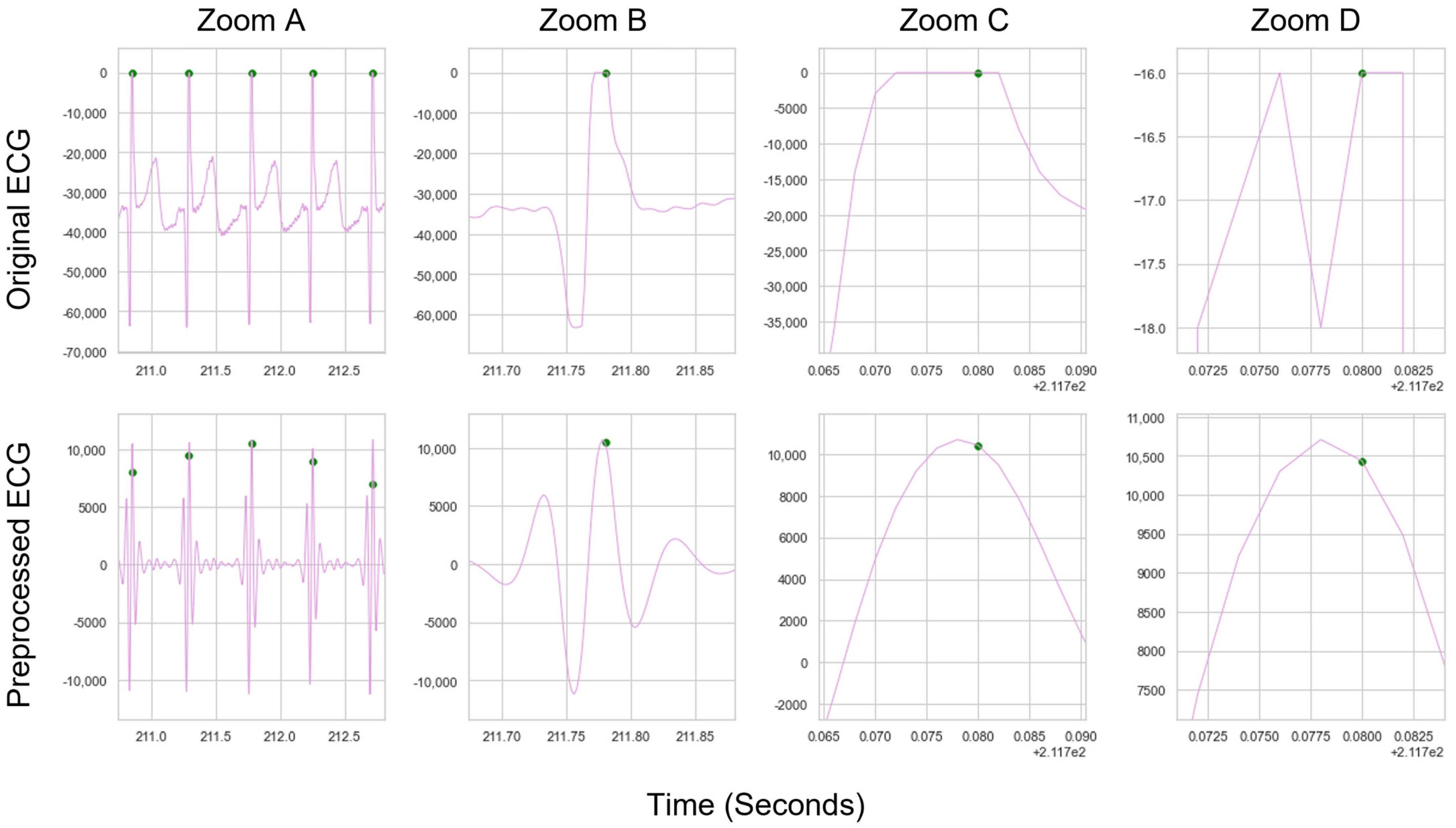
Once the signal has undergone preprocessing, the resulting preprocessed ECG contains R-peak locations that differ slightly from the raw ECG, due to the mathematical operations that occur during preprocessing. In order to readjust the peaks back to the original location on the raw ECG (i.e., the R-peak location on the raw ECG, rather than the R-peak location on the preprocessed ECG), we introduce a “local peak-correction” operation. Additionally, we introduce a square wave specific filter for those devices where it is appropriate.

2.2.1. Existing ECG Approaches

Firstly, 12 open source pre-existing ECG methods (

Table 2. A guide to the pre-existing ECG pipelines tested in this study.

ECG Method	Method Description
HeartPy [36,42,43]	Designed for noisy data. Preprocessing uses baseline wander removal, a 0.05 Hz notch filter, and a 0.003–20 Hz bandpass filter. Peak detection uses an adaptive threshold, then outlier detection and rejection. HeartPy user-customisation is used to raise the maximum allowed HR to 220 bpm.
Neurokit2 [44]	Preprocessing uses only a 0.5 Hz HPF and a 50 Hz notch filter. Gradients are used to detect QRS complexes, then an R-peak is detected within each QRS.
Pan-Tompkins [45]	Preprocessing uses a 5–15 Hz BPF before taking a derivative, squaring, and integrating with a moving window to isolate the R-Peak, which is detected via a series of thresholds.
Hamilton [33]	Adaptation of the Pan–Tompkins method that uses an 8–16 Hz BPF rectification instead of squaring, and also a smaller integration window.
Christov [29]	Uses two self-adjusting algorithms to detect the current beat and the interval between beats, self-adjusting for different sampling frequencies. It is particularly designed for multi-lead analysis.
Engelse & Zeelenberg [46,47] (EngZee)	Uses a 48–52 Hz notch filter differentiates the signal, passes it through an adaptive LPF, and then uses Christov-inspired adaptive threshold analysis to detect the peak.
Kalidas [35]	Resamples the signal to 80 Hz; uses Daubechies 3 wavelets for stationary wavelet transforms. The signal is squared and a moving window average enhances the R-peaks, which are detected using threshold-based peak detection.
Nabian [32]	R-peak detection derived from Pan–Tompkins. A sliding window is used to detect a liberal initial R-peak list before culling the list.
Martinez [37,48]	Aims to identify multiple ECG complexes. Uses a quadratic spline wavelet transform to identify the QRS peak.
Elgendi [28]	Uses an 8–20 Hz BPF along with moving window integration and thresholding to detect the R-peaks.
Zong [31]	Uses a 16 Hz LPF, a non-linear scaling factor to enhance the QRS complex and reduce low-frequency noise, and then adaptive thresholds to determine the onset and duration of the QRS complex.
Rodrigues [30]	Uses a double derivative, square, and moving window integration in preprocessing to enhance the QRS complex. A finite-state machine enhances the R-peak position [49], with an adaptive exponential decaying threshold for R-peak detection [50].

) were applied to Datasets A and B. These approaches represented the available open source methods for R-peak extraction. Based on an investigation of open source approaches, three separate Python packages that contained all or a subset of these methods were initially considered—HeartPy, Neurokit2, and py-ecg detectors. However, all ECG methods in py-ecg detectors were found to contain matching implementations in Neurokit2, without the flexibility to implement preprocessing and the peak detection of a method separately. This reduced the selection of ECG methods to those found in the HeartPy and Neurokit2 packages—the default HeartPy method and 11 other approaches from the Neurokit2 package (including the default Neurokit2 approach). The open source nature of Neurokit2 meant that some methods may match more closely than others to the authors’ original intentions. Almost all methods within the Neurokit2 package were tested, but some were excluded. A sum-slope approach [40] was initially tested but then excluded due to very poor performance (to the point that including it in the analysis made it hard to visualise the other results). An approach by Koka and Muma [41] relied on visibility graphs, but was much slower than other methods, requiring an additional package to work. Two methods did not successfully run when tested within the Neurokit2 framework: an approach by Gamboa [34] and a Probabilistic Methods Agreement via Convolution (ProMAC) approach, which combined the results of other peak-detection methods. The ProMAC method, which relies on other approaches, likely failed because the Gamboa method also failed. Aside from these exclusions, which were made for reasons of performance, our analysis captured all open source approaches to R-peak labelling in ECGs within common Python packages. It is acknowledged that proprietary measures for measuring infant ECGs may well exist as part of commercial innovations and research.

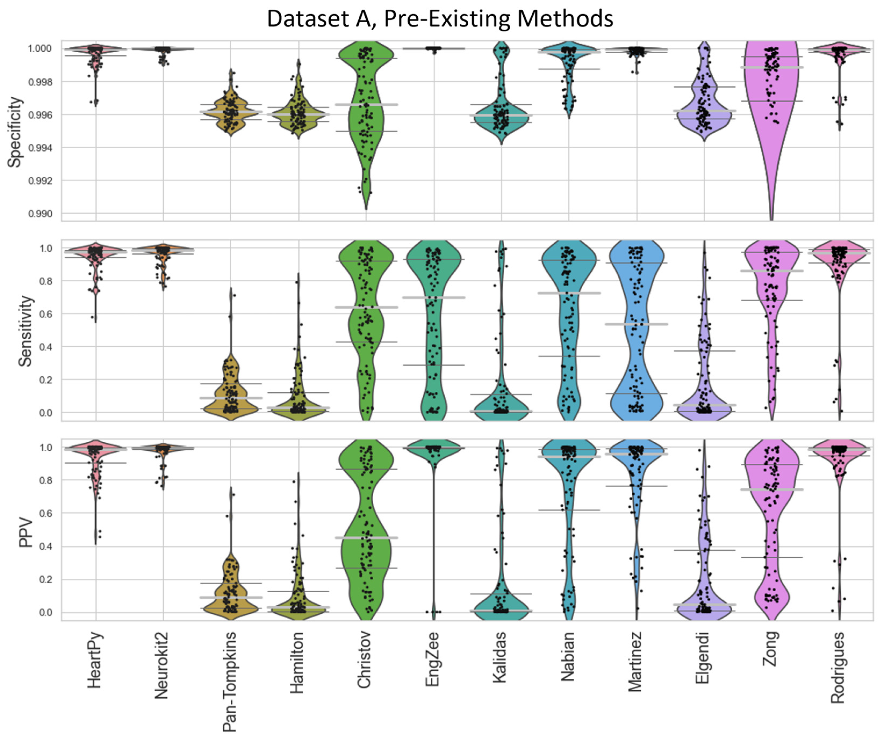
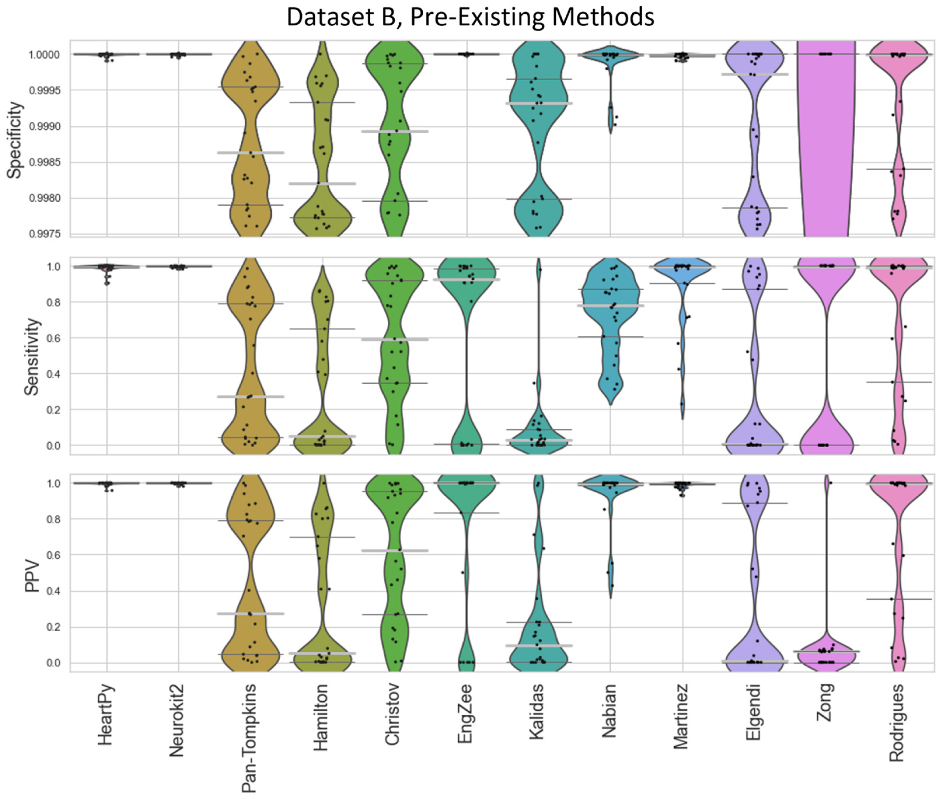
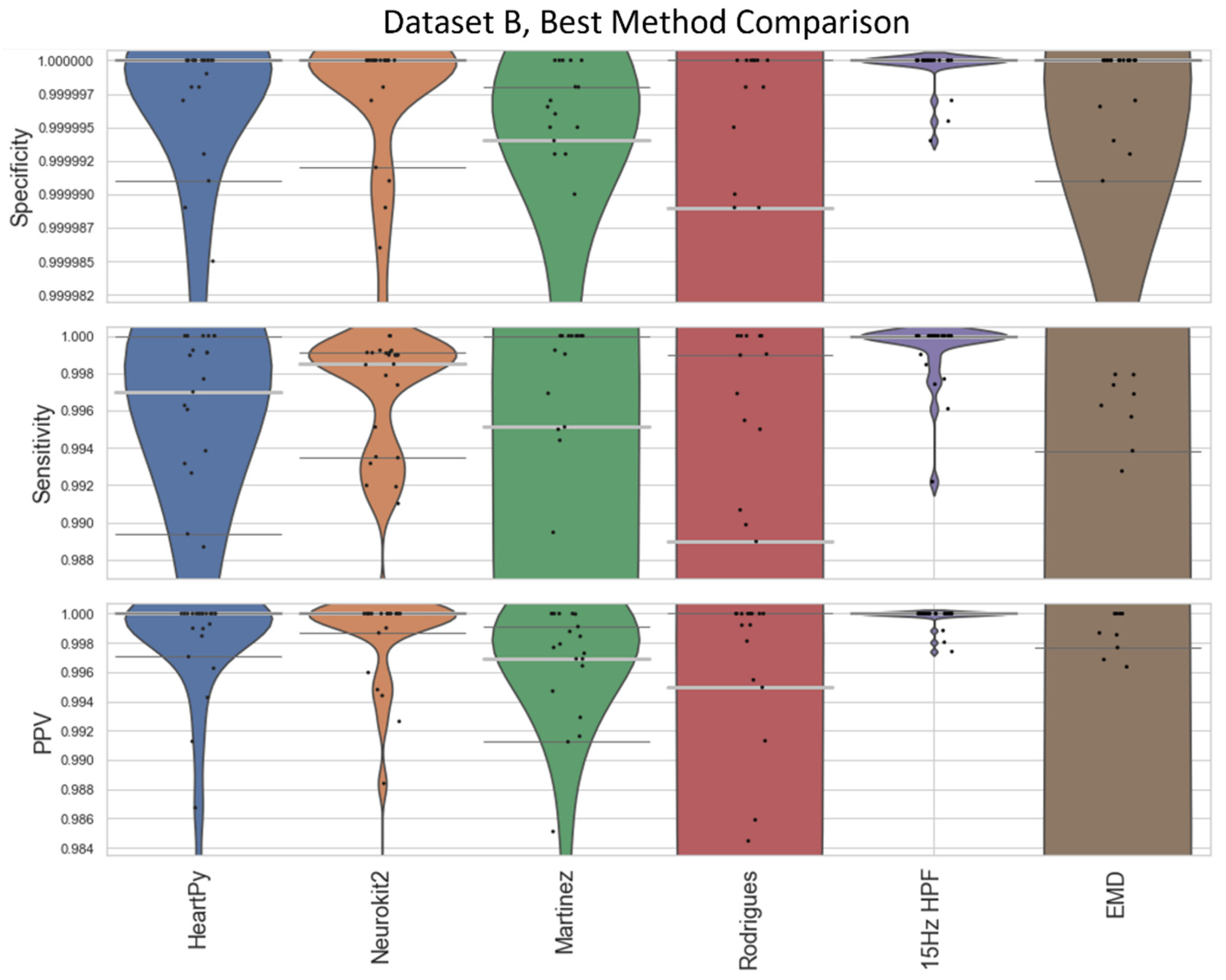
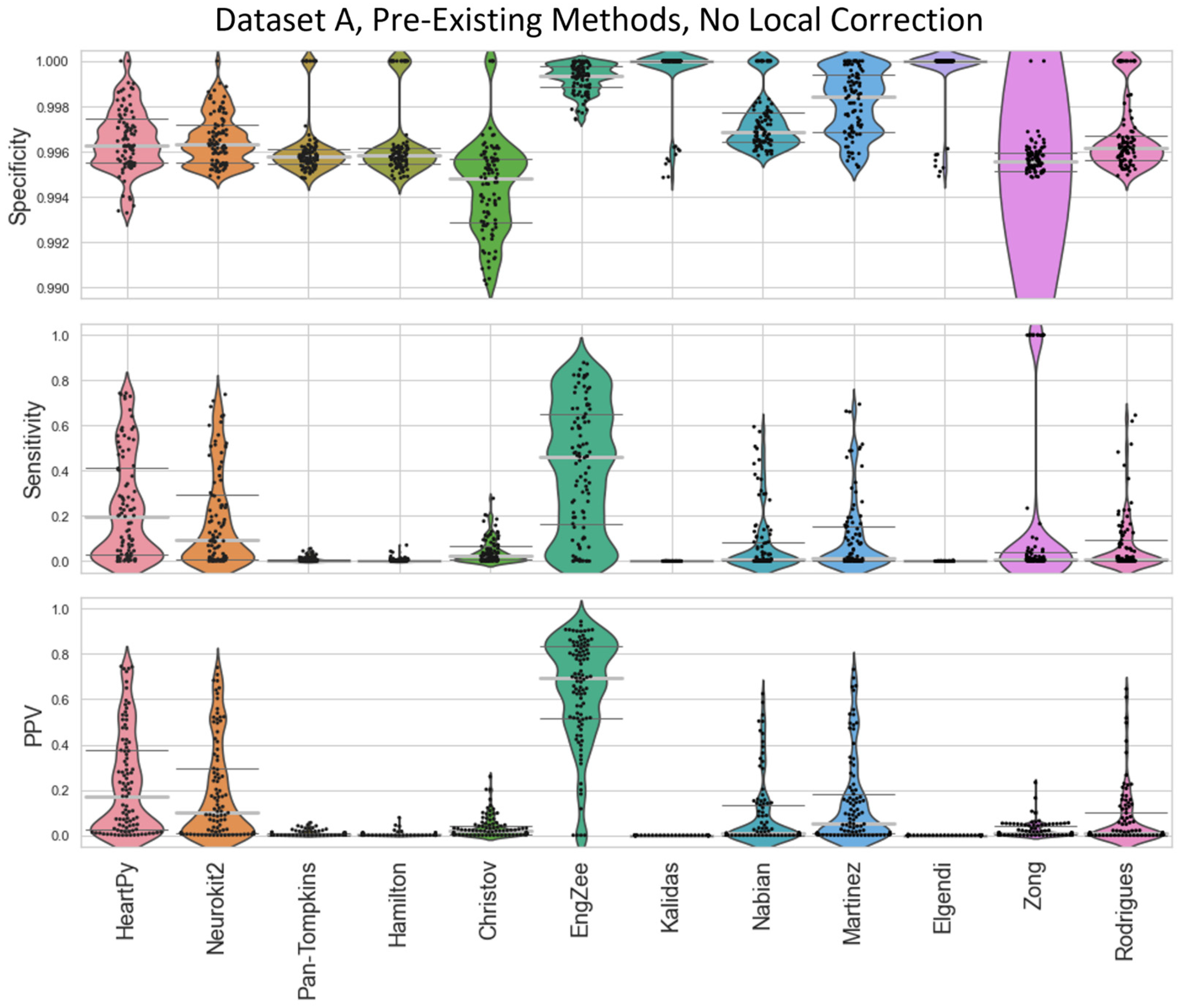
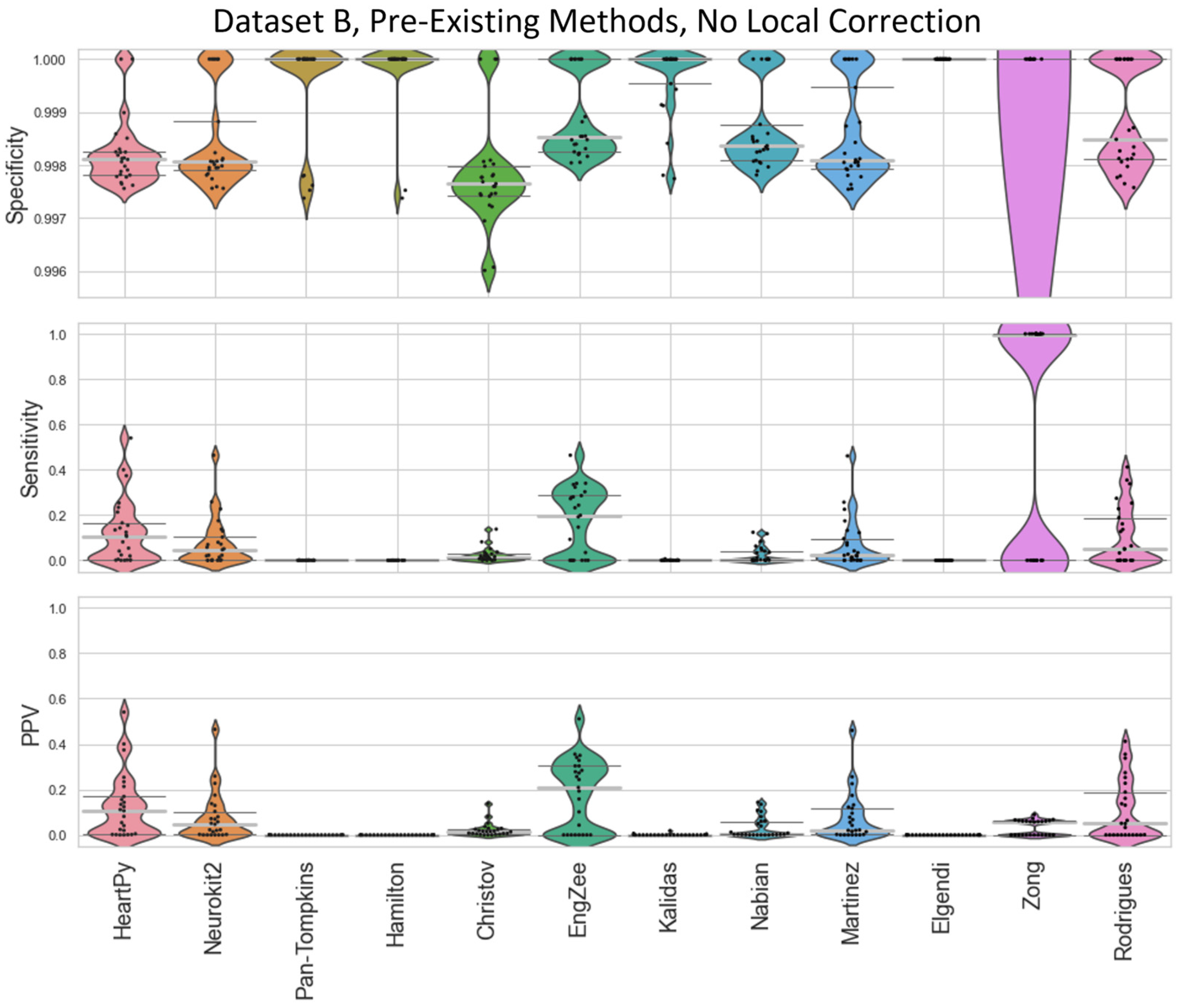
The specificity, sensitivity, and positive predictive value (PPV) of the methods were then compared against a ground truth set of labels (Figure 4 and Figure 5). Specificity penalises incorrect peak selection, and PPV identifies the ratio of correctly identified peaks out of all the peaks identified for a given method. Given the sparsity of peaks within a signal, both measures tend to be preferable due to their inclusion of false positives within the denominator. The sensitivity is also important but can be falsely inflated by a method identifying many false peaks, and so must be considered in the context of the other two metrics. These methods all require the precise detection of peak location.

Specificity = (True Negatives)/(True Negatives + False Positives)

(2)

Sensitivity = (True Positives)/(True Positives + False Negatives)

(3)

Positive Predictive Value = (True Positives)/(True Positives + False Positives)

(4)

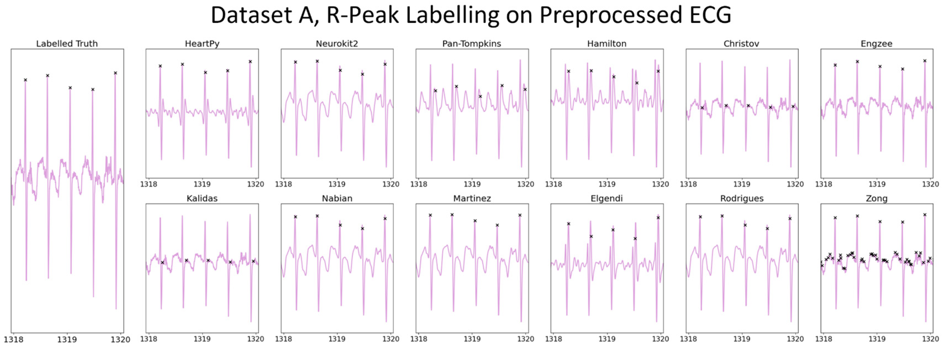
The distributions of the results are shown in violin plots, with black dots representing each individual result. The median and interquartile ranges (IQRs) are also shown as dotted lines. Collectively, this visualisation allows for the evaluation of both the summative statistics and the general metric distribution. In cases where the results of some methods fall far beyond the range of the best-performing methods, visualisations are truncated to present a clearer comparison between the core performances. For each method, conventional preprocessing was applied, although a local peak correction was used after labelling to allow a fair comparison between the different methods. The datasets used were Datasets A and B, which were both clean enough to have a reliable ground truth. A visualisation of the algorithmically labelled peaks by different methods in a sample infant ECG without local peak correction is shown in Figure 6, with the labels shown on both the preprocessed ECGs.

The range of successes that different current methods have for dealing with infant ECGs are shown for Dataset A (Figure 4) and Dataset B (Figure 5). Figure 6’s visualisation shows the effect of different preprocessing methods on the raw heart rate, and that some approaches label other complexes in the ECG instead of the QRS.

The inbuilt methods for both the Neurokit2 package [44] and HeartPy package [36] outperformed the implementation of all other pre-existing methods, with the Neurokit2 method performing best between the two. This was true when considering their respective full distribution, median, or interquartile ranges (IQRs). Out of the remaining methods, Martínez et al.’s wavelet-based method [48] and Rodrigues et al.’s approach [30] were 3rd and 4th best respectively. Martínez’s method had good specificity and fairly good PPVs but worse sensitivity, indicating the peaks that were detected were accurate, but many peaks were missing. Rodrigues’s method was able to adapt better than most methods to the fast heart rate and noisy signals, but still had some worst-case subjects that it was unable to adapt to, especially in Dataset B.

Nabian et al.’s method [32] performed 5th-best overall, narrowly outperforming the sensitivity of Martínez’s method for Dataset A, but had more results with poorer for specificity and PPV. Zong’s approach [31] did next best for Dataset A, but fell apart completely for Dataset B. Engelse and Zeelenberg’s method [46,47] had a low false-peaks-detection rate, but also did not detect enough of the true peaks for an accurate HR calculation. Christov’s method [29] seemed to work well with some of the signals but needed the altering of its internal threshold factors to properly adapt to the children’s ECGs.

All other approaches tested [28,33,34,35] did not perform well with the datasets and had lower median specificity/sensitivity/PPV values than the other methods. They likely need some fundamental changes to be suited to the ECG of a young child, as many of these methods have time constraints that work very well for adults but are too rigid for the faster heart rate of a child, falsely rejecting too many R-peaks or identifying other complexes in the ECG over the QRS complex.

2.2.2. Proposed ECG Preprocessing

We developed two separate preprocessing approaches by adapting the best-performing pre-existing approach (Neurokit2). These two approaches were a frequency-preprocessing approach and an empirical mode decomposition (EMD) approach, which were both then tested and compared against the existing approaches. The frequency-based approach applies filters that attenuate the energy of a signal occurring at a given frequency. Low-pass filters (LPFs) remove high-frequency detail, only allowing smooth changes in the signal to pass through. High-pass filters (HPFs) do the opposite, removing smooth signal trends to leave more rapidly altering complexes in the signal. Bandpass filters (BPFs) remove some of the high-frequency and low-frequency information, whereas notch filters only remove signal energy at a given frequency. One problem with frequency filters is that they do not discriminate between two separate signal sources that share a frequency band. EMD is an adaptive technique that decomposes the signal into intrinsic mode functions (IMFs)—characteristic signals that can have an overlapping frequency information [51]. If noise or non-QRS complexes can be completely captured in an IMF, they can be removed without affecting the QRS. This same logic can also be applied to wavelet filtering [37,52,53].

A recent study [54] found that a 0.05–150 Hz BPF preprocessing approach outperformed a 1–17 Hz BPF approach on a study investigating peak detection in children—but the study only tested those two specific filters. As such, it was considered worth evaluating a range of 5th-order Butterworth BPFs and HPFs applied before R-peak detection.

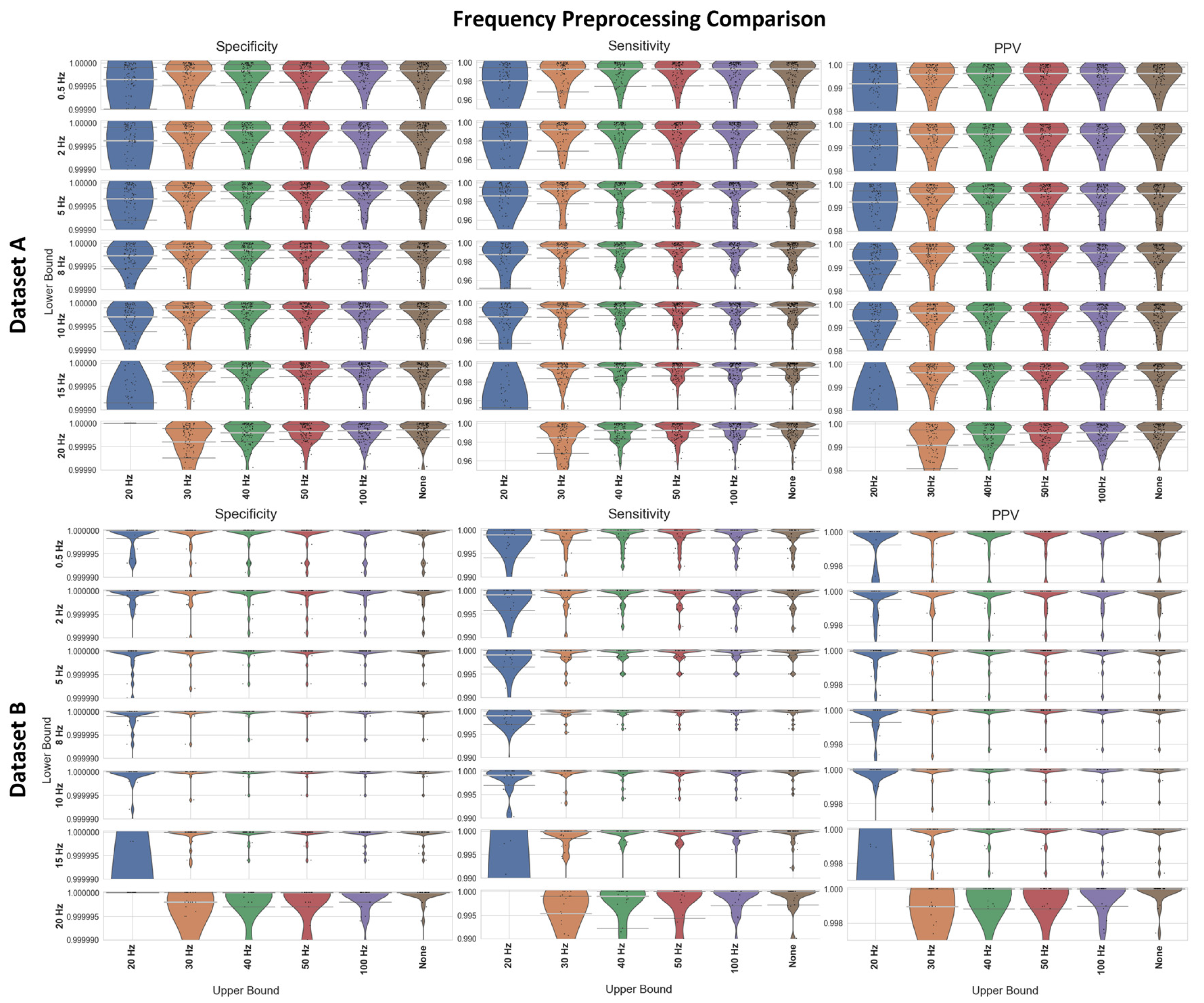
We chose the Neurokit2 algorithm for peak detection due to its high performance across all categories (Figure 4 and Figure 5) as well as the simplicity of the initial baseline Neurokit2 preprocessing (a 0.5 Hz HPF with a 50 Hz band stop filter). A variety of different frequency filters were applied in addition to the standard Neurokit2 preprocessing to determine the best frequency-preprocessing approach. Dataset A and Dataset B were both used to test the frequency ranges (Figure 7). Upper frequency bounds of 20, 30, 50, 100, and “None” were used (with the “None” option indicating no upper bound, i.e., a pure HPF). A range of lower bounds was also tested, with 0.5, 2, 5, 8, 10, 15, and 20 Hz lower bounds shown in Figure 7. All filters were 5th-order Butterworth filters. In general, the high-pass filters had better median specificity/sensitivity/PPV than the bandpass filters, as well as overall improved distributions. However, the improvement in the results is marginal when compared to the 50 Hz/100 Hz upper bounds. For Dataset A, the 15 Hz HPF approach was marginally better than similar filter approaches when considering median and IQR values, although an upper bound of 50 Hz and any lower bound in the range of 8–20 Hz produced fairly similar results. For Dataset B, the lower IQR had perfect specificity, sensitivity, and PPV for the 5–15 Hz HPF, with the only distinguishing factor being how well the worst-case results were processed. However, the 20 Hz HPF results were a lot worse for Dataset B.

During the assessment of the ECG preprocessing options, elevated T-waves were observed in some of the subjects in the recordings. T-waves typically overlap in frequency with QRS waves [55], which can cause some problems in R-peak detection. An approach using EMD can remove the T-waves while preserving the QRS complex. Here, we removed any signals with >50% of the signal power in the range of 0.5–8 Hz, given that the T-wave content was reported to lie in the 0–10 Hz range [55], and the QRS was reported to lie in the 8–20 Hz range [28]. The EMD approach was also used with standard Neurokit2 preprocessing and peak detection.

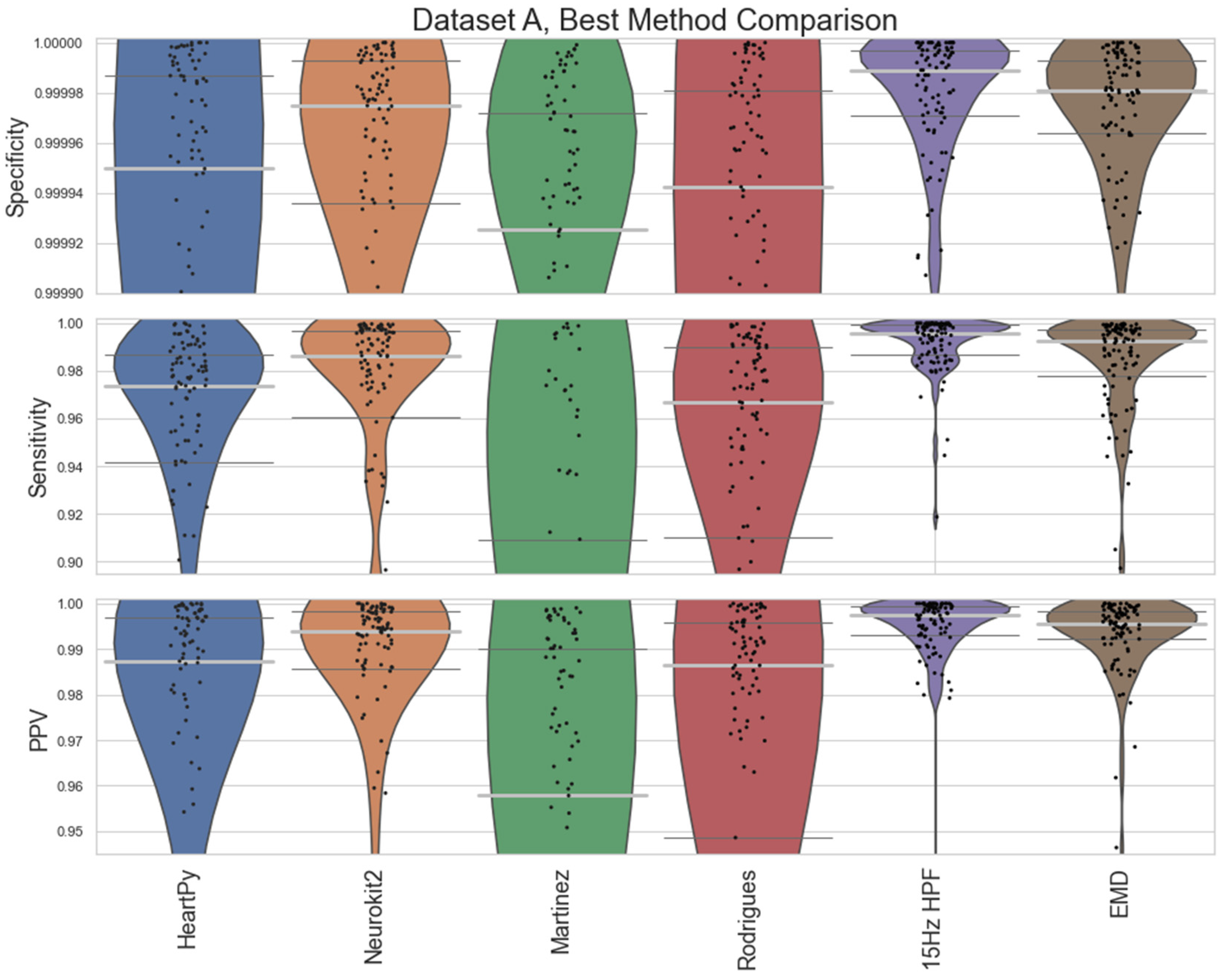
A comparison between the proposed 15 Hz HPF filter and the EMD approach with the best-performing pre-existing approaches is shown in Figure 8 (Dataset A) and Figure 9 (Dataset B). The HeartPy, Neurokit2, Martinez, and Rodrigues results display the same characteristics as in Figure 4 and Figure 5. The 15 Hz HPF approach improves on the EMD and all pre-existing methods in terms of worst-case labelling and median/IQR statistics for Dataset A. Specifically, the 15 Hz HPF median specificity, sensitivity, and PPV (0.999989, 0.9958, and 0.9975, respectively) outperformed the median results of all other methods, the closest pre-existing method being Neurokit2 (0.999975, 0.9863, 0.9938). If we interpret these median results on the average signal length (30.5 min, 4180 peaks), it means 13 fewer peaks were labelled incorrectly (10 vs. 23), 39 fewer peaks were missed (18 vs. 57), and only 0.25% of peaks that were identified were labelled incorrectly (vs. 0.72% for Neurokit2). While the EMD approach does improve on the other pre-existing approaches for Dataset A, for Dataset B, the EMD approach performs much worse overall, with a few worst-case labels performing very poorly.

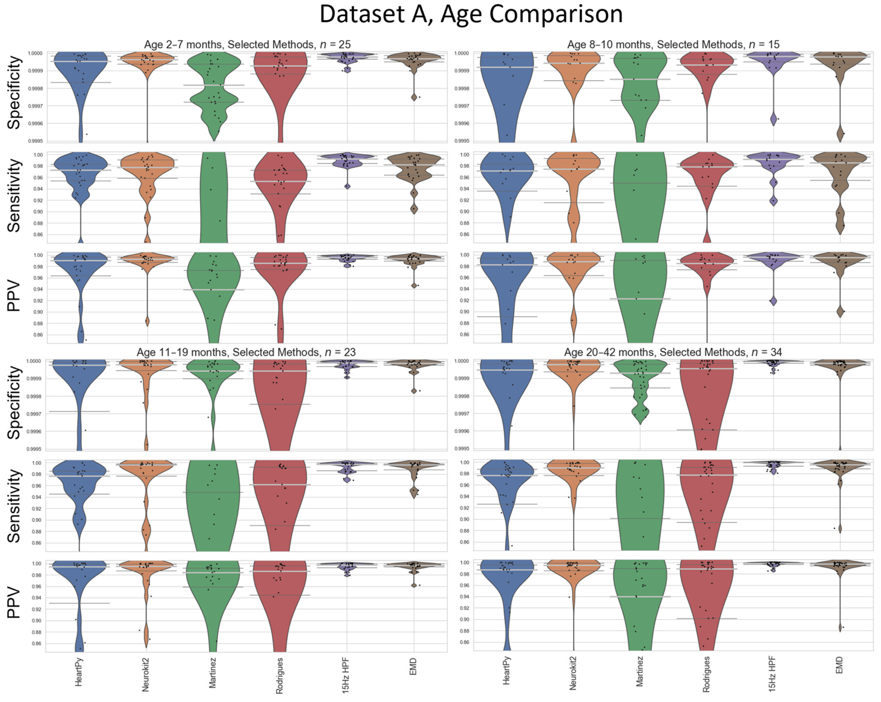
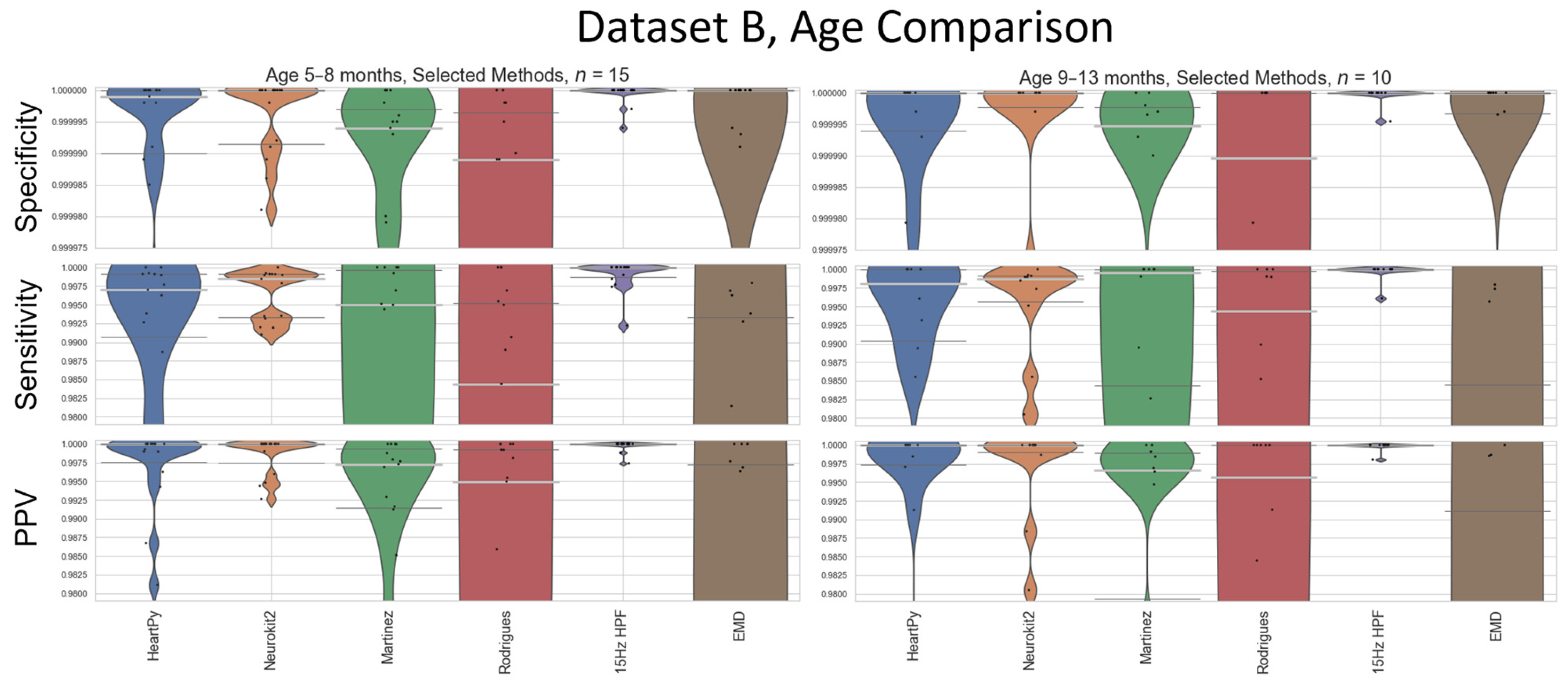
Average heart rate varies as a function of age [16], so a sub-analysis visualising the performance of the methods at different age boundaries on Dataset A is also carried out (Figure 10). Age-divisions were chosen as a balance between keeping a large enough cohort size for a valid analysis, and to recognise natural groupings that arose within the datasets (Figure 3). Dataset B’s age-based analysis contained far fewer participants, especially when split into cohorts, and is included in Appendix C for completeness. The results for the 15 Hz HPF on Dataset A are the worst in the 8–10 month age range, but still outperform all other methods at all age ranges (Figure 10).

2.2.3. ECG Peak Detection

R-peak detection is the process by which an algorithm finds the R-peak within the QRS complex for all QRS complexes in an ECG signal. By testing all the pre-existing methods, it was clear that Neurokit2 was one of the best suited to these datasets (Figure 4 and Figure 5) and worked well with the proposed preprocessing approaches of 15 Hz HPF or EMD filtering (Figure 7 and Figure 8). Neurokit2 peak detection was used in the proposed ECG pipeline without alteration in this specific step.

2.2.4. Local Peak Correction

Stronger frequency filtering applied during the preprocessing step had a stronger impact on peak location, shifting R-peaks (and other peaks) in the ECG (Figure 6). To counteract the shifting-peaks effects, we implemented a novel local correction relative to the unfiltered signal. This correction iteratively searches for the largest peak ± 0.01 s either side of the peak location on the processed ECG to check for a larger local peak within the raw unprocessed ECG, until no larger peak is found within the search limit. To distinguish this technique from “peak detection”, it is referred to as “peak correction”. This peak correction only has a small impact on peak location but preserves variations between peaks and allows for a more accurate comparison of specificity/sensitivity/positive predictive value measures (Appendix D). In instances where multiple indices could be labelled for a given peak, the closest peak to the preprocessed ECG was used (Appendix E).

It was also observed that the first and last beats of an ECG were liable to be missed under certain methods. This was addressed by a one-second artificial extension of the signal at the start and the end. The first/last values of the preprocessed ECG were used as the constant values for the extensions at each end. While this only has a small impact for long recordings, it can be very impactful for shorter recordings.

2.2.5. Square Wave Peak Correction

While filter-based preprocessing deals with many sources of noise, any periodic non-ECG signal is likely to be preserved with the frequency-processing and EMD methods. Square waves were occasionally observed when recording was started prior to attaching the device to a subject. The nature of square waves is very likely dependent on the device, and square wave removal is highly recommended in these recordings. For the EgoActive sensor (University of York, UK) responsible for Dataset C, a median filter with a 101 sample width was used to exclude blocks of signals that were within 0.5% of a local maximum/minimum. The precise filter width and max/min margins depended on the gain and the sampling rate of the device used. This correction was applied post-peak detection to remove any peaks deemed to occur during these periods. Square wave correction was not required for Datasets A and B.

2.3. The HR Pipeline

2.3.1. Raw Heart Rate Calculation

Once a set of R-peaks is detected, the heart rate can be calculated as described by Equation (1). This is an instantaneous heart rate calculation reflecting beat-to-beat changes. For some research questions, an average heart rate (collected over a few beats) will be preferred and will likely reduce the impact of noise in the calculation. Here, only instantaneous heart rate was considered. Even with good R-peak-detection methods, a peak can be missed or a non-R-peak can be incorrectly labelled. This leads to an erroneous heart rate measurement, which can be detected using filtering.

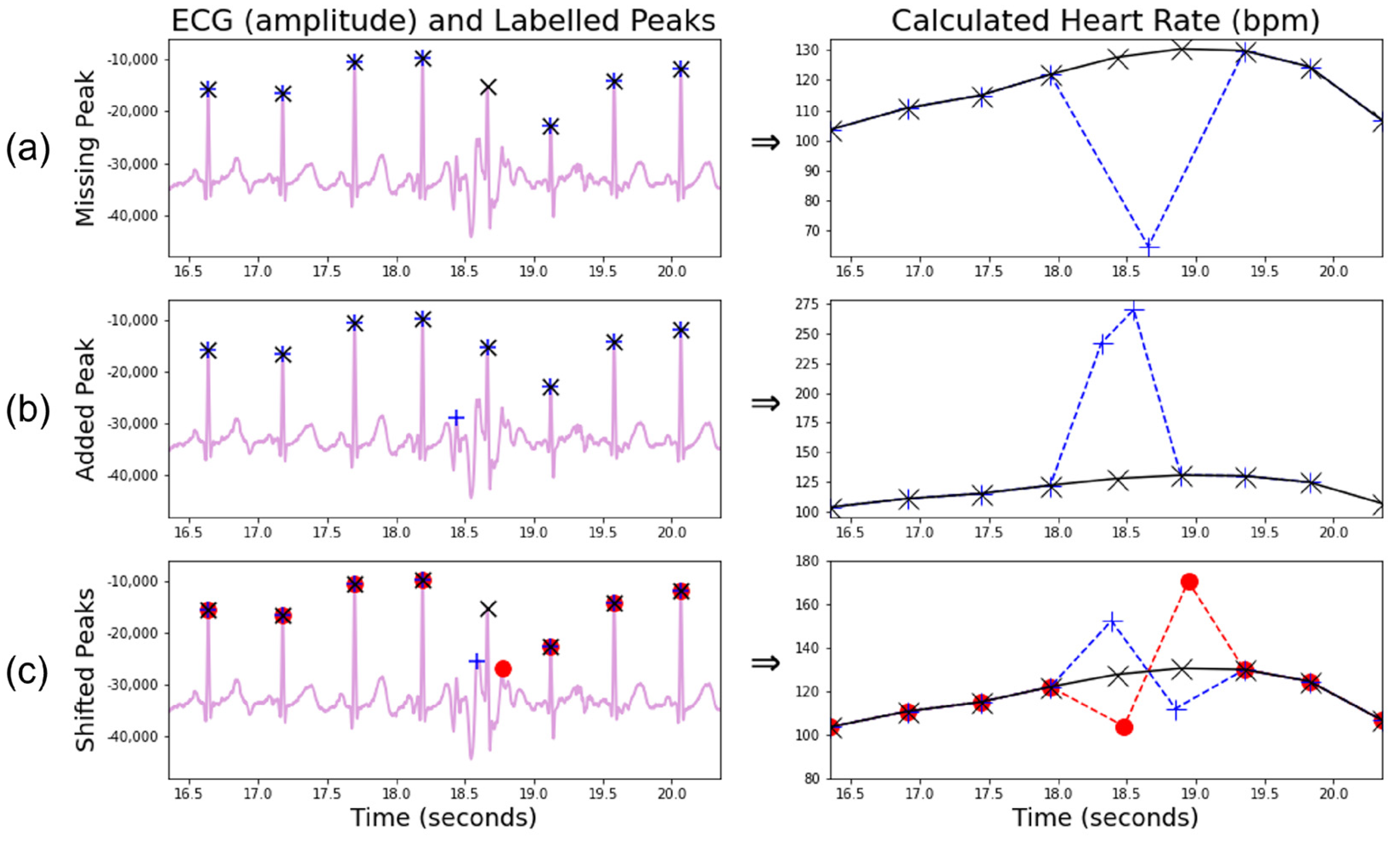
2.3.2. Correction for Missing and Additional Beats

A missing R-peak causes two true measurements to be replaced by a single false measurement of approximately half value (Figure 11a), while an additional peak causes one true measurement to be replaced by two roughly double-false measurements (Figure 11b), although the proximity of the additional peak to existing peaks alters the amplification ratio of the subsequent heart rate.

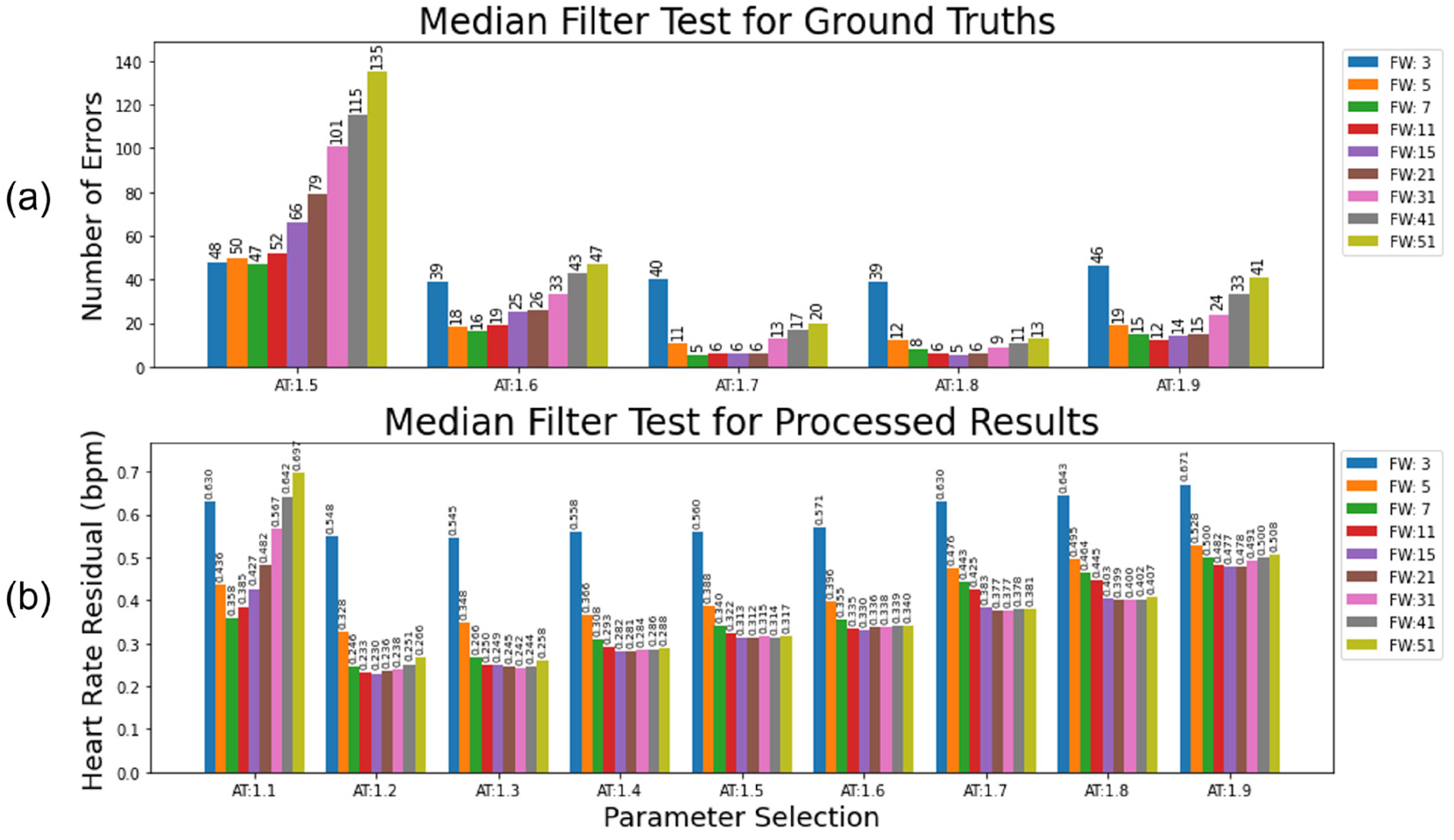
Two metrics were used to ascertain the ideal filter width and proportional threshold for HR processing. The first metric was used to evaluate the median approach applied to a clean set of R-peak labels that only contained a few errors. The second metric was used to evaluate the median approach applied to a realistically processed ECG.

Dataset A (n = 97) was captured using a BiosignalPlux device (PLUX Biosignals, Lisbon, Portugal) that recorded the ECG with Bluetooth. Across the 97 recordings, occasional disconnections occurred, leading to gaps in the signal (23 in total). Additionally, the noise arising from infant motion also led to short periods where no QRS complex could be identified (323). These gaps in the ground truth R-peak list resulted in drops in the derived HR signal. The optimal median filter approach identifies these gaps without removing any real signal. The expected number of gaps to interpolate over was recorded for each participant. The absolute difference between interpolations made by the filter and the expected number of interpolations was used to evaluate the optimal parameters for a clean environment. Figure 12a shows the variation in these results with different parameter choices.

Next, the output from the proposed ECG pipeline (15 Hz HPF preprocessing, Neurokit2 peak detection) was used to represent a realistically preprocessed signal. The residual heart rate between the median-filtered ECG and a ground truth (with gaps interpolated over) was used to demonstrate the optimal parameters from a noisier baseline (Figure 12b).

For the clean ECG test (Figure 12a), a high activation threshold (e.g., 1.7 or 1.8) combined with a narrow filter width (e.g., 7–21) produced a very low number of incorrect adjustments (<3% compared to the total number of adjustments or <0.0015% compared to every potential adjustment, e.g., every single heart rate beat). Almost all these incorrect adjustments were due to arrhythmias in the heart rate, causing a longer than expected gap between the detected beats. A very conservative threshold combined with very few beats needed to accurately determine the incorrect label made sense, given the cleanness of the ground truth. For the test with the processed ECG (Figure 12b), a much more liberal activation threshold (e.g., 1.2 or 1.3) with a much wider filter width (15–31) provided the optimal parameters for reducing the heart rate residual with this dataset. This accounted for the higher level of uncertainty in the underlying truth in the processed heart rate.

2.3.3. Correction for Shifted Beats

Wrongly located R-peaks can remain undetected by the median filter approach described above. A useful observation is that an early labelled beat leads to a much greater heart rate rise followed by a much steeper heart rate drop than typically appears in a natural signal (Figure 11c). A late-labelled beat does the opposite. The proposed algorithm searches for the presence of three consecutive sign changes concurrently with a large variation in the heart rate difference (>15 bpm for the first and third heart rate gaps, >25 bpm for the middle gap), thus identifying the mislabelled beats within a signal, provided the neighbouring beats are correct. Areas with large amounts of mislabelled beats are likely to be caught by the algorithm for missing/additional beats and are likely one reason for the more conservative thresholds present In the processed HR tests.

2.3.4. Signal Quality Index Calculation

In addition to developing methods to correct R-peak labels for longform infant ECGs, it is important to identify time periods that have many (consecutive) incorrect labels due to noisy measurements. Local linear interpolation is unable to accurately reflect the underlying HRs for these periods, and so they may need to be excluded from further data analyses. Thus, we developed an algorithm optimised for longform infant ECGs to help identify regions in which a data recovery approach was inadvisable.

Pre-existing methods for HR quality assessment were not found to be suitable for long heart rates, and all of them were tuned on adult datasets. Kramer et al. [56] used a non-stationary signal, viable heart rate range, and high signal-to-noise ratio (SNR), but required the signal to be rejected/accepted in full. Rodrigues et al. [20] extracted shapes and behaviours of the signal to group ECG samples by an agglomerative clustering approach, an approach that becomes computationally inefficient for longer recordings. It is also worth noting that many SQI methods implicitly try to reject areas of high noise directly in the ECG [57]. The HeartPy method [36] explicitly rejects peaks that create a beat interval >30% above or below the mean interval time of the whole signal. Li et al. [58] used local kurtosis based on expected kurtosis values for ECG and common ECG noise sources. Bizzego et al. [59] rejected peaks if the R-peak maxima was not followed by an S-trough minima at least 70% of the local (1 s wide) range of the signal. Additionally, Zhao and Zhang [60] proposed a noise-detection algorithm based on an agreement from different ECG algorithms. However, given the results in this paper showing the poor performance of most algorithms on infant ECGs (Figure 4 and Figure 5), this approach was not explored here.

The beat correction algorithm for missed/additional beats was used as a baseline measure of signal quality, with additional steps added to fine-tune the quality algorithm further. Figure 2 highlights that correctly labelled R-peaks typically fall inside the expected bounds, whereas incorrectly labelled R-peaks are likely going to either cause a steep decrease or increase in heart rate (for missing or additional labels, respectively). By calculating the proportion of “wrong” labels within a given filter width, a rolling measure of heart rate signal quality was calculated. If a small number of incorrect labels was present, a close approximation to the original heart rate could be recovered. If many measurements were incorrect, then the heart rate could not be reliably approximated. A filter width of 31 and an adaptive threshold of 1.3 were used (Figure 12b).

A moving-median approach was used to create the base of a binary signal quality index (SQI) vector [13]. At each time point (i.e., heartbeat measurement), the percentage of local beats within the filter width that deviated by a multiplicative factor of 1.3 above or below the local median was calculated (i.e., the local median indicated the existence of a poor signal within the sliding window, and for a median HR of 100 bpm, the proportion of beats outside the range of 77–130 bpm was calculated). If the percentage of poor beats was ≤25%, then SQI = 1 (high signal quality) at that time point. Otherwise, SQI = 0 (low signal quality). The sliding window was then moved to the next time point. This multiplicative factor was similar to the value reported by Bizzego et al. [59], which used outlier detections from the median of the five most recent “correctly labelled” HR values.

To make the SQI more accurate, additional manipulations were used to account for the specific locations of the high-deviation beats. First, the regions of good SQIs were then extended (i.e., set to SQI = 1) according to whether the beats just beyond the boundary of the good SQI region were within the local median range. Second, continuous regions >3.5 s long of high-deviation beats (>1.3 beats from local median) were set to SQI = 0, as were any gaps in the heart rate longer than 2.5 s. Lastly, any remaining good regions <5 s long were set to SQI = 0 to leave regions of a reasonable size. These parameters could be tailored depending on the length of the useful heart rate region for a given research question, and how precise a heart rate was required to be.

The Boolean SQI vector can then be applied to the heart rate by either setting areas of bad signal to 0 bpm, or by cutting those regions from the signal.

2.3.5. SQI-Filtered Heart Rate

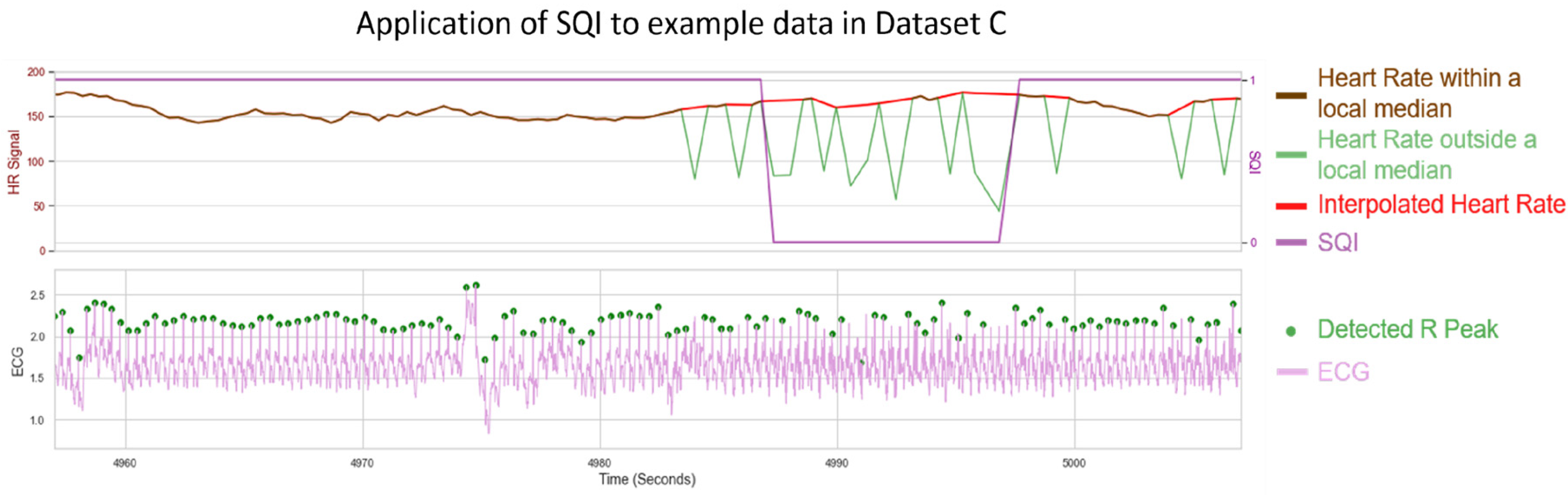
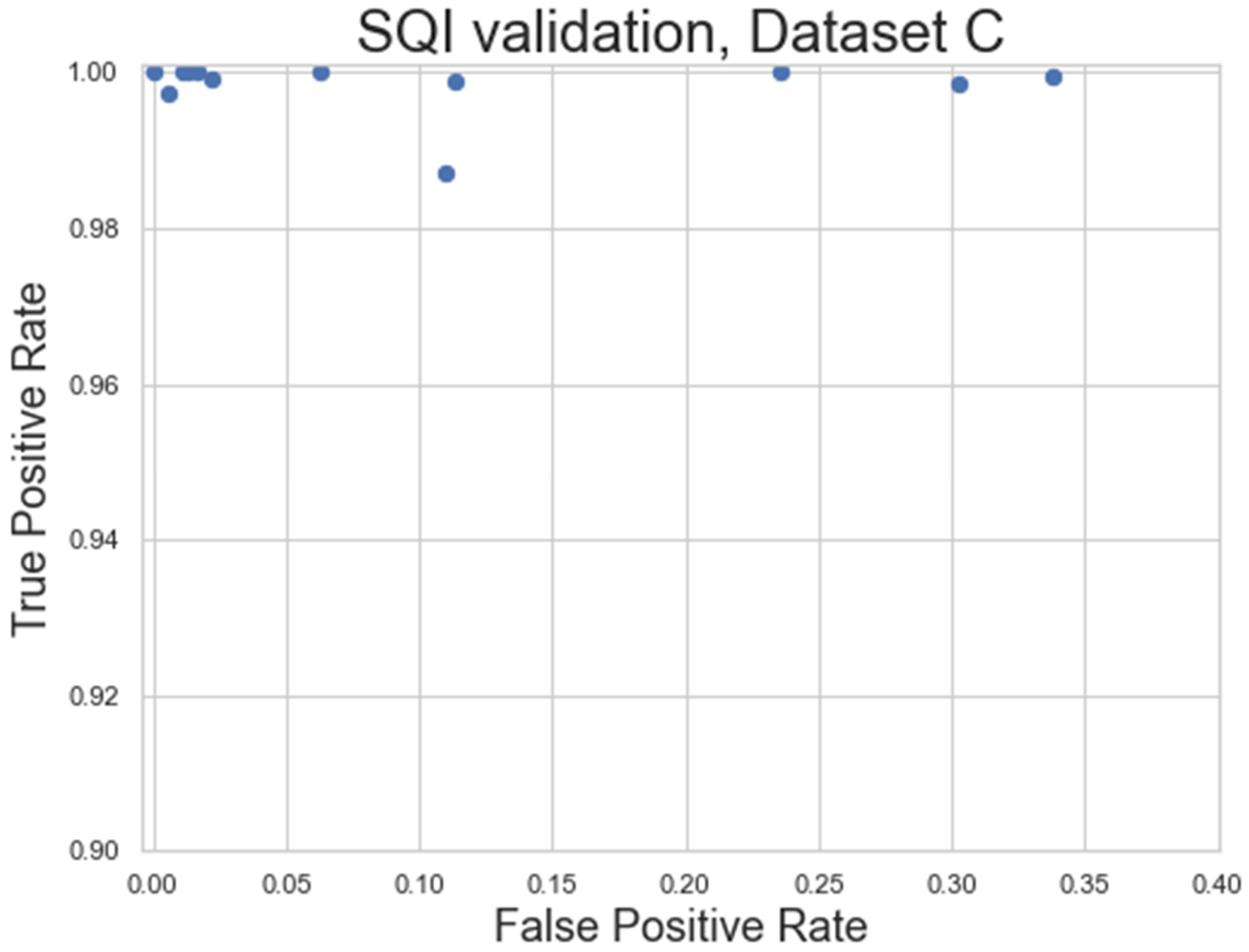
The SQI step of the pipeline was evaluated using the specificity and sensitivity metrics (Equations (2) and (3)) applied to Dataset C, a very longform dataset (length ≥ 50 min) captured outside of a lab environment, taken at 250 Hz. These factors were combined to provide high levels of noise in the dataset, while still being clean enough to have areas of signal that should be preserved. A set of filtering parameters that minimised the residual error in the processed HR (AT: 1.3, FW: 31) were used as the base for the SQI algorithm (Figure 12b). An example visualisation of the SQI algorithm applied to a noisy HR is shown in Figure 13, with the results of the analysis shown in Figure 14.

As seen in Figure 13, the SQI algorithm is not designed to label an HR signal as poor where only individual beats are missing. However, where multiple peaks are missing and the underlying median filter is more unreliable, the HR is designed to be labelled as not usable. Figure 14 shows the general success rate of the SQI algorithm when applied to noisy datasets. Overall, the SQI has a high true positive rate, meaning almost no clean signal is excluded from the recording. The SQI has a higher false positive rate for some of the recordings, meaning some noisy signals can make it into the final analysis, which may require these recordings to be excluded. However, this does represent a significant improvement over the baseline of including all HR signals and is also shown to work very well for the cleaner signals (top left in Figure 14).

2.3.6. Cleaned and Filtered Heart Rates

The end result is a heart rate signal that has been corrected in areas of small mislabelling, and is discounted in large areas of noise where the signal is unrecoverable.

3. Discussion

To date, there has been limited research on ECG R-peak-detection methods which are adequate for infants. In this paper, existing open source ECG methods were tested on infant datasets acquired in a range of conditions (including naturalistic conditions), and the best-performing method was adapted into a high-performing novel pipeline that contained all the necessary steps from raw ECG preprocessing to HR calculation.

The strengths of our proposed approach include: (1) improving preprocessing and local peak-correction steps; (2) explicitly outlining a guide for when to interpolate missing/additional beats; and (3) introducing an SQI vector designed to detect unreliable areas of HR measurements that can be adapted for further data analysis steps. These strengths make our ECG pipeline particularly relevant for real-world large datasets collected in the natural environment, where the manual rejection of unreliable areas of HR measurements is not feasible. The first strength also improves infant ECG analysis specifically, an area in which we demonstrate the current existing open source approaches to fall short. Additionally, we ensured the entire process was computationally efficient and did not depend on any commercial software in order to maximise ease of use.

Both the HeartPy and Neurokit2 packages are highly useful open source scientific tools that collectively provide a wide range of options for ECG analysis. They both provide a wide range of functionality beyond R-peak detection in ECGs, although that is all we focussed on here. It is worth acknowledging that there are many methods that exist outside of the open source domain that are not evaluated here. While many of the methods in Neurokit2 were open source, originally some were written in different languages and had to be adapted into Python, with both the translation issues and the inherent nature of open source collaborative approaches meaning that some imperfections in implementations could arise. The analysis in this paper focused on the available open source implementation of these methods, rather than the methods themselves.

The HeartPy and Neurokit2 default methods showed the best results with Dataset A and Dataset B overall, with both performing particularly well on Dataset B. The Rodrigues method performed well on Dataset A, and Martinez showed good specificity and a reasonably good PPV IQR on Dataset A and a good overall performance on Dataset B. All four approaches were quick to run and had ECGs that they labelled to a very high standard, although all of them also had ECGs that were not labelled as accurately as our proposed pipeline managed later.

The inbuilt Neurokit2 method was chosen as a candidate for further fine tuning due to the high performance and simple initial preprocessing. Many existing methods contain several hard-coded parameters that have been developed to work with adult ECGs. Neurokit2′s inbuilt method only used a notch filter tuned at the mains frequency and a conservative high-pass filter of 0.5 Hz. Neurokit2 preprocessing was applied before all frequency-processing testing, but the specific notch filter could be altered depending on the ECG device, and the 0.5 Hz HPF could also be removed, given that a stronger HPF is likely to be optimal for an infant ECG.

In developing a new pipeline, it was found that a 15 Hz HPF provided an approximate best filter for infant ECG preprocessing (Figure 7), which was very different to the 8–20 Hz BPF commonly suggested for preprocessing in adults [28]. This held for two different devices with different amounts of subject motion and different sampling rates (Figure 8 and Figure 9). It also improved on other methods at a range of age ranges (Figure 10). While the specific bands were slightly different for the two datasets (e.g., a 20 Hz HPF worked well for Dataset A but not Dataset B), the 15 Hz HPF fell within a good range both times. This gives us confidence that it is a more robust methodology for infants. It would be interesting for a future study to test the age range at which the optimal HPF begins to drop for older children. The precise frequency bounds used could vary slightly depending on the specific device used and sample population. These results indicate that any upper bound of 50 Hz or higher and any lower bound of 8–15 Hz appear to have very similar levels of performance across both tested datasets.

The proposed EMD preprocessing approach improved the default Neurokit2 method slightly in Dataset A but did not outperform the optimal frequency-processing filter. In Dataset B, there were a few worst-case scenarios that caused the EMD approach to have low specificity and PPV. Additionally, there was a dramatically increased run-time when applying EMD processing. As such, it is not recommended to use this approach.

One major contribution of the new pipeline is the novel local peak correction. The 0.01 s threshold was determined heuristically to balance overcoming high-frequency noise while minimising false peak detection. This allowed for much heavier filtering without compromising the R-peak label locations, as well as a comparative analysis between R-peak detections for the different methods. The start/end peak detections had a very minimal reactive effect, and the start/end of ECGs were often discarded. However, in pure detection terms, it was found to improve all the open source algorithms evaluated here at a very low computational cost, and so is recommended for future inclusion. Square wave filtering was device-specific, as two thirds of the devices detected did not tend to exhibit square wave noise, and so square wave filtering only succeeded in subtracting noise from the signal. However, for the device that did exhibit square wave noise, it greatly improved the detection results.

Where either precise beat detection is required or a heart is suspected to contain arrhythmias, the heart rate filtering proposed here may not be appropriate. However, it was found to perform a good job at preserving the overall shape of the heart rate, and subsequently served as a good way to detect noisy periods when also combined with the SQI. It was found that a much more conservative activation threshold (1.7/1.8) and thinner width of the median filter (7–15) were optimal for cleaner ECGs, but that more liberal thresholds (1.2/1.3) and wider filters (15–31) produced lower residual heart rates when applied to the detected heart rate (Figure 12). While it is recommended to view some raw ECGs along with the processed heart rates to ascertain the underlying level of noise, a choice of 1.7/11 or 1.3/31 activation thresholds/filter widths for cleaner and noisier signals, respectively, can serve as a fair initial parameter choice (with the former being recommended for short lab-based ECGs with no motion, and the latter being recommended for any other forms of ECG).

Neither Datasets A nor B were sufficiently noisy to test the SQI analysis properly. As such, Dataset C was the only one used for this purpose. The sensor used for Dataset C was the EgoActive sensor (University of York, UK), a lightweight wearable device designed for much longer recordings in the natural environment, while being as unobtrusive as possible to the child to ensure comfort and allow free movement. The lower ECG sampling rate (250 Hz) was chosen to maximise the duration of a continuous recording [13]. The SQI approach to determine noisy periods of HR served as a good first step towards a robust noise-detection algorithm. The SQI-mediated HR allowed for the analysis of long recordings, which could contain large amounts of noise. While the SQI method serves as a good automatic way to identify unreliable heart rate calculations, the specific parameters used depend on the research question. For example, a more noise-averse analysis, such as standard deviation-based HRV, requires stricter noise thresholds. Analyses concerned with general HR rises/falls or average HRs can use a looser threshold to capture more data. The SQI calculation worked very well on recordings with easily discernible noise, being particularly good at separating non-HR periods from HR periods, but struggled a bit more with noisy HRs vs. clean HRs. Understanding and automatically detecting which types of noise cause a poorer performance can make it more robust in future studies. The specific parameters used in the SQI are dependent on how much noise is tolerable for a given research problem, meaning it will likely have to be double-checked if the parameters are altered.

The proposed pipeline was very computationally efficient. The ECG pipeline was applied to all of Dataset A (n = 97, sampling rate = 500 Hz, M_recording = 32 min, 94,089,683 data points) and took 111.33 s in total (1.15 s per ECG). The total preprocessing and peak labelling time was 20.75 s (0.21 s per ECG) and the local peak correction took 90.59 s (0.93 s per ECG). The HR pipeline is also computationally efficient, as a combination of median filters and difference functions provide the backbone for both the SQI and the beat-cleaning algorithms. By applying the SQI to the heart rate, the size of the vectors processed are greatly reduced compared to an ECG (1–3 Hz sample density for HR compared to 250–1000 Hz for ECG). A separate n = 63 set of noisy HR signals collectively covering 92 h (comprising 559,612 beats in total) took only a 6.68 s total processing time. This included both the time to filter the heart rate with a moving-median filter and the time to create the SQI vector. All calculations were performed consecutively using an 11th Gen Intel(R) Core (TM) i5–1145G7 @ 2.60 GHz and did not include the loading times required to import the data into Python initially.

3.1. Limitations

The research carried out here tested the performance of existing open source approaches on an infant ECG dataset. There are other approaches not included in these open source packages that can show improved performances on infant datasets, and the nature of open source software means that these approaches are susceptible to change. This research was carried out on version 0.2.3 of Neurokit2 and version 1.2.6 of HeartPy. Version 1.1.1 of PyEMD was used for the EMD analysis.

An additional limitation of the Neurokit2 peak-detection method was that heart rates faster than 200 bpm were often mislabelled (with only alternate peaks being detected). It is rare, but not impossible, for an infant heart rate to exceed 200 bpm, and so care must be taken if this occurs.

As is usual with the filtering methodology, our HR pipeline is also dependent on filter selection. We accounted for this by verifying the effect of different parameters on clean and noisy HR signals and generated a set of optimal parameters for both scenarios. Additionally, the pipeline was developed on a typically developing population without known cardiac issues. An ECG containing a lot of arrhythmias or other HR irregularities may not be suitable for an automated cleaning approach carried out in this manner. Similarly, the SQI portion of the heart rate pipeline is also dependent on tuning parameters.

Finally, while we endeavoured to label a ground truth, there was some fundamental uncertainty regarding R-peak locations in noisy ECGs. Noise is exacerbated in free-moving individuals and such a movement is often heightened in infants. While we did our best to adjust for this uncertainty (see Appendix B and Appendix E), it must be considered alongside the results.

3.2. Future Research

Since adaptations are shown to improve the Neurokit2 pipeline, it is very possible that other methods can also be adapted to process infant ECGs. Additionally, the Neurokit2 package is being continually updated and the interaction of newer methods [61] with infant ECGs should be considered. Some exploratory analyses of the HeartPy and Pan–Tompkins methods were carried out and were not initially encouraging (though they were not in-depth enough to draw concrete conclusions). Additionally, while the computational inefficiency of the EMD approach was a concern for longform ECGs, many studies have focused on shorter infant ECG signals where the processing time was less of a factor. Given the strong performance of the approach on Dataset A, it is very possible that small alterations in the EMD methodology (such as the criteria for IMF rejection) can prove to be a positive avenue for future research.

The datasets captured here lay the groundwork for a future infant-specific approach for R-peaks, especially for machine-learning approaches. Additionally, they could also be of great use in future infant-specific analysis of the remaining ECG morphology.

Infants have fast heart rates, and their movements and activities can add substantial noise to ECGs. Our method was developed particularly to address these issues for infant ECG recordings. However, our pipeline can be adapted for other applications in which researchers may need to deal with noisy data. For example, the pipeline was adapted by using a different high-pass filter in preprocessing (e.g., 0.5 Hz vs. 15 Hz) to allow the whole pipeline to work with adults [13]. It could be informative to acquire ECG recordings from a range of ages (e.g., 3–18 year olds) to further test our pipeline to account for different heart rate speeds [16] and investigate developmental trajectory through ECG recordings. Finally, further testing is needed to investigate the performance of the HR SQI and peak-correction algorithms on atypical heart rates (e.g., arrhythmias).

Finally, sensor orientation and position, particularly for small wearable sensors, can have a great impact on different infant ECG complexes. A general analysis creating a consistent set of guidelines for wearable infant ECGs can be of great use to the scientific community, as can further validations of different aspects of this pipeline on the data collected at specific sensor orientations and positions.

4. Conclusions

In this work, we evaluated existing open source ECG pipelines on longform infant datasets, before improving the state-of-the art approach to develop our own pipeline. We also developed an HR pipeline to clean up the signal and identify areas that were too noisy to process. Collectively, these formed a full, computationally-efficient pipeline to turn raw infant ECG signals into cleaned and processed HR signals. This process is designed to even work on naturalistic recordings, although it also outperforms existing methods in short lab-based recordings of infants. The use of the algorithms developed here on three separate datasets provide evidence for their robustness across a range of ECG devices. Importantly, these algorithms will increase confidence in future infant ECG research, particularly for longform ECG datasets collected outside the lab where infants can exhibit natural behaviours.

References

1. Fox, N.A.; Schmidt, L.A.; Henderson, H.A.; Marshall, P.J. Developmental Psychophysiology: Conceptual and Methodological Issues. In Handbook of Psychophysiology; Cacioppo, J.T., Tassinary, L.G., Berntson, G., Eds.; Cambridge University Press: Cambridge, UK, 2007; pp. 453–481. [Google Scholar] [CrossRef]
2. Porges, S.W.; Raskin, D.C. Respiratory and heart rate components of attention. J. Exp. Psychol. 1969, 81, 497–503. [Google Scholar] [CrossRef]
3. Richards, J.E.; Casey, B.J. Heart Rate Variability During Attention Phases in Young Infants. Psychophysiology 1991, 28, 43–53. [Google Scholar] [CrossRef]
4. Zantinge, G.; van Rijn, S.; Stockmann, L.; Swaab, H. Physiological Arousal and Emotion Regulation Strategies in Young Children with Autism Spectrum Disorders. J. Autism Dev. Disord. 2017, 47, 2648–2657. [Google Scholar] [CrossRef]
5. Zantinge, G.; van Rijn, S.; Stockmann, L.; Swaab, H. Psychophysiological responses to emotions of others in young children with autism spectrum disorders: Correlates of social functioning. Autism Res. 2017, 10, 1499–1509. [Google Scholar] [CrossRef]
6. Gomez, I.N.; Flores, J.G. Diverse Patterns of Autonomic Nervous System Response to Sensory Stimuli among Children with Autism. Curr. Dev. Disord. Rep. 2020, 7, 249–257. [Google Scholar] [CrossRef]
7. Heilman, K.J.; Harden, E.R.; Zageris, D.M.; Berry-Kravis, E.; Porges, S.W. Autonomic regulation in fragile X syndrome. Dev. Psychobiol. 2011, 53, 785–795. [Google Scholar] [CrossRef]
8. Cheng, Y.C.; Huang, Y.C.; Huang, W.L. Heart rate variability in individuals with autism spectrum disorders: A meta-analysis. Neurosci. Biobehav. Rev. 2020, 118, 463–471. [Google Scholar] [CrossRef]
9. Imeraj, L.; Antrop, I.; Roeyers, H.; Swanson, J.; Deschepper, E.; Bal, S.; Deboutte, D. Time-of-day effects in arousal: Disrupted diurnal cortisol profiles in children with ADHD. J. Child Psychol. Psychiatry Allied Discip. 2012, 53, 782–789. [Google Scholar] [CrossRef] [PubMed]
10. Van Goozen, S.H.M.; Matthys, W.; Cohen-Kettenis, P.T.; Buitelaar, J.K.; Van Engeland, H. Hypothalamic-pituitary-adrenal axis and autonomic nervous system activity in disruptive children and matched controls. J. Am. Acad. Child Adolesc. Psychiatry 2000, 39, 1438–1445. [Google Scholar] [CrossRef]
11. Mulkey, S.B.; dú Plessis, A. The Critical Role of the Central Autonomic Nervous System in Fetal-Neonatal Transition. Semin. Pediatr. Neurol. 2018, 28, 29–37. [Google Scholar] [CrossRef]
12. Groome, L.J.; Swiber, M.J.; Atterbury, J.L.; Bentz, L.S.; Holland, S.B. Similarities and Differences in Behavioral State Organization during Sleep Periods in the Perinatal Infant before and after Birth. Child Dev. 1997, 68, 1–11. [Google Scholar] [CrossRef]
13. Geangu, E.; Smith, W.A.P.; Mason, H.T.; Martinez-Cedillo, A.P.; Hunter, D.; Knight, M.I.; Liang, H.; Garcia de Soria Bazan, M.d.C.; Tse, Z.T.H.; Rowland, T.; et al. EgoActive: Integrated Wireless Wearable Sensors for Capturing Infant Egocentric Auditory–Visual Statistics and Autonomic Nervous System Function ‘in the Wild’. Sensors 2023, 23, 7930. [Google Scholar] [CrossRef]
14. Maitha, C.; Goode, J.C.; Maulucci, D.P.; Lasassmeh, S.M.S.; Yu, C.; Smith, L.B.; Borjon, J.I. An open-source, wireless vest for measuring autonomic function in infants. Behav. Res. Methods 2020, 52, 2324–2337. [Google Scholar] [CrossRef]
15. Dahl, A. Ecological Commitments: Why Developmental Science Needs Naturalistic Methods. Child Dev. Perspect. 2017, 11, 79–84. [Google Scholar] [CrossRef]
16. Fleming, S.; Thompson, M.; Stevens, R.; Heneghan, C.; Plüddemann, A.; MacOnochie, I.; Tarassenko, L.; Mant, D. Normal ranges of heart rate and respiratory rate in children from birth to 18 years of age: A systematic review of observational studies. Lancet 2011, 377, 1011–1018. [Google Scholar] [CrossRef]
17. Lackner, H.K.; Eglmaier, M.T.W.; Hackl-Wimmer, S.; Paechter, M.; Rominger, C.; Eichen, L.; Rettenbacher, K.; Walter-Laager, C.; Papousek, I. How to use heart rate variability: Quantification of vagal activity in toddlers and adults in long-term ecg. Sensors 2020, 20, 5959. [Google Scholar] [CrossRef]
18. Alcantara, J.M.A.; Plaza-Florido, A.; Amaro-Gahete, F.J.; Acosta, F.M.; Migueles, J.H.; Molina-Garcia, P.; Sacha, J.; Sanchez-Delgado, G.; Martinez-Tellez, B. Impact of using different levels of threshold-based artefact correction on the quantification of heart rate variability in three independent human cohorts. J. Clin. Med. 2020, 9, 325. [Google Scholar] [CrossRef]
19. Tipple, M. Interpretation of Electrocardiograms in Infants and Children. Images Paediatr. Cardiol. 1999, 1, 3–13. Available online: http://www.ncbi.nlm.nih.gov/pubmed/22368537 (accessed on 11 November 2022).
20. Rodrigues, J.; Belo, D.; Gamboa, H. Noise detection on ECG based on agglomerative clustering of morphological features. Comput. Biol. Med. 2017, 87, 322–334. [Google Scholar] [CrossRef]
21. Li, H.; Boulanger, P. An automatic method to reduce baseline wander and motion artifacts on ambulatory electrocardiogram signals. Sensors 2021, 21, 8169. [Google Scholar] [CrossRef]
22. Clifford, G.D. ECG Statistics, Noise, Artifacts, and Missing Data. In Advanced Methods and Tools for ECG Data Analysis; Artech. House Inc.: London, UK, 2006. [Google Scholar]
23. Friesen, G.M.; Jannett, T.C.; Jadallah, M.A.; Yates, S.L.; Quint, S.R.; Nagle, H.T. A Comparison of the Noise Sensitivity of Nine QRS Detection Algorithms. IEEE Trans. Biomed. Eng. 1990, 37, 85–98. [Google Scholar] [CrossRef]
24. Fariha, M.A.Z.; Ikeura, R.; Hayakawa, S.; Tsutsumi, S. Analysis of Pan-Tompkins Algorithm Performance with Noisy ECG Signals. J. Phys. Conf. Ser. 2020, 1532, 012022. [Google Scholar] [CrossRef]
25. Tanasković, I.; Miljković, N. A new algorithm for fetal heart rate detection: Fractional order calculus approach. Med. Eng. Phys. 2023, 118, 104007. [Google Scholar] [CrossRef]
26. Matonia, A.; Jezewski, J.; Kupka, T.; Jezewski, M.; Horoba, K.; Wrobel, J.; Czabanski, R.; Kahankowa, R. Fetal electrocardiograms, direct and abdominal with reference heartbeat annotations. Sci. Data 2020, 7, 200. [Google Scholar] [CrossRef]
27. Zhang, Y.; Yu, S. Single-lead noninvasive fetal ECG extraction by means of combining clustering and principal components analysis. Med. Biol. Eng. Comput. 2020, 58, 419–432. [Google Scholar] [CrossRef]
28. Elgendi, M.; Jonkman, M.; Deboer, F. Frequency bands effects on QRS detection. In Proceedings of the BIOSIGNALS 2010-Proceedings of the Third Internsational Conference on Bio-inspired Systems and Signal Processing, Valencia, Spain, 20–23 January 2010; pp. 428–431. [Google Scholar] [CrossRef]
29. Christov, I.I. Real time electrocardiogram QRS detection using combined adaptive threshold. Biomed. Eng. Online 2004, 3, 28. [Google Scholar] [CrossRef] [PubMed]
30. Rodrigues, T.; Samoutphonh, S.; Silva, H.; Fred, A. A low-complexity R-peak detection algorithm with adaptive thresholding for wearable devices. In Proceedings of the 2020 25th International Conference on Pattern Recognition (ICPR), Milan, Italy, 10–15 January 2021; pp. 9967–9974. [Google Scholar] [CrossRef]
31. Zong, W.; Moody, G.B.; Jiang, D. A robust open-source algorithm to detect onset and duration of QRS complexes. In Proceedings of the Computers in Cardiology, Thessaloniki, Greece, 21–24 September 2003; pp. 737–740. [Google Scholar] [CrossRef]
32. Nabian, M.; Yin, Y.; Wormwood, J.; Quigley, K.S.; Barrett, L.F.; Ostadabbas, S. An open-source feature extraction tool for the analysis of peripheral physiological data. IEEE J. Transl. Eng. Health Med. 2018, 6, 1–11. [Google Scholar] [CrossRef]
33. Hamilton, P.S. Open Source ECG Analysis. Comput. Cardiol. 2002, 29, 101–104. [Google Scholar]
34. Gamboa, H. Multi-Modal Behavioral Biometrics Based on HCI and Electrophysiology. Ph.D. Thesis, Universidade Tecnica de Lisboa, Lisbon, Portugal, 2008. [Google Scholar]
35. Kalidas, V.; Tamil, L.S. Real-time QRS detector using stationary wavelet transform for automated ECG analysis. In Proceedings of the 2017 IEEE 17th International Conference on Bioinformatics and Bioengineering (BIBE), Washington, DC, USA, 23–25 October 2017; pp. 457–461. [Google Scholar]
36. van Gent, P.; Farah, H.; van Nes, N.; van Arem, B. HeartPy: A novel heart rate algorithm for the analysis of noisy signals. Transp. Res. Part F Traffic Psychol. Behav. 2019, 66, 368–378. [Google Scholar] [CrossRef]
37. Li, C.; Zheng, C.; Tai, C. Detection of ECG Characteristic Points Using Wavelet Transforms. IEEE Trans. Biomed. Eng. 1995, 42, 21–28. [Google Scholar] [CrossRef] [PubMed]
38. Pal, S.; Mitra, M. Empirical mode decomposition based ECG enhancement and QRS detection. Comput. Biol. Med. 2012, 42, 83–92. [Google Scholar] [CrossRef]
39. Velayudhan, A.; Peter, S. Noise Analysis and Different Denoising Techniques of ECG Signal—A Survey. IOSR J. Electron. Commun. Eng. (IOSR-JECE) 2016, 3, 40–44. [Google Scholar]
40. Carreiras, C.; Alves, A.P.; Lourenço, A.; Canento, F.; Silva, H.; Fred, A. BioSPPy: Biosignal Processing in Python. 2015. Available online: http://biosppy.readthedocs.org/ (accessed on 8 March 2024).
41. Koka, T.; Muma, M. Fast and Sample Accurate R-Peak Detection for Noisy ECG Using Visibility Graphs. In Proceedings of the Annual International Conference of the IEEE Engineering in Medicine and Biology Society, EMBS, Glasgow, UK, 11–15 July 2022; pp. 121–126. [Google Scholar] [CrossRef]
42. van Gent, P. Python Heart Rate Analysis Toolkit Documentation. 2020. Available online: https://github.com/paulvangentcom/heartrate_analysis_python (accessed on 15 October 2021).
43. van Gent, P.; Farah, H.; van Nes, N.; van Arem, B. Analysing Noisy Driver Physiology Real-Time Using Off-the-Shelf Sensors: Heart Rate Analysis Software from the Taking the Fast Lane Project. J. Open Res. Softw. 2019, 7, 1–9. [Google Scholar] [CrossRef]
44. Makowski, D.; Pham, T.; Lau, Z.J.; Brammer, J.C.; Lespinasse, F.; Pham, H.; Schölzel, C.; Chen, S.H.A. NeuroKit2: A Python toolbox for neurophysiological signal processing. Behav. Res. Methods 2021, 53, 1689–1696. [Google Scholar] [CrossRef]
45. Pan, J.; Tompkins, W.J. A real-time QRS detection algorithm. IEEE Trans. Biomed. Eng. 1985, 32, 230–236. [Google Scholar] [CrossRef]
46. Engelse, W.A.H.; Zeelenberg, C. Single Scan Algorithm for QRS-Detection and Feature Extraction. Comput. Cardiol. 1979, 6, 37–42. [Google Scholar]
47. Lourenço, A.; Silva, H.; Leite, P.; Lourenço, R.; Fred, A. Real time electrocardiogram segmentation for finger based ECG biometrics. In Proceedings of the BIOSIGNALS-2012-International Conference on Bio-Inspired Systems and Signal Processing, Vilamoura, Portugal, 1–4 February 2012; pp. 49–54. [Google Scholar] [CrossRef]
48. Martínez, J.P.; Almeida, R.; Olmos, S.; Rocha, A.P.; Laguna, P. A Wavelet-Based ECG Delineator Evaluation on Standard Databases. IEEE Trans. Biomed. Eng. 2004, 51, 570–581. [Google Scholar] [CrossRef]
49. Sadhukhan, D.; Mitra, M. R-Peak Detection Algorithm for ECG using Double Difference And RR Interval Processing. Procedia Technol. 2012, 4, 873–877. [Google Scholar] [CrossRef]
50. Gutiérrez-Rivas, R.; García, J.J.; Marnane, W.P.; Hernández, Á. Novel Real-Time Low-Complexity QRS Complex Detector Based on Adaptive Thresholding. IEEE Sens. J. 2015, 15, 6036–6043. [Google Scholar] [CrossRef]
51. Huang, N.E.; Shen, Z.; Long, S.R.; Wu, M.C.; Shih, H.H.; Zheng, Q.; Yen, N.-C.; Chao Tung, C.; Liu, H.H. The Empirical Mode Decomposition and the Hilbert Spectrum for Nonlinear and Non-Stationary Time Series Analysis. 1998. Available online: https://www.jstor.org/stable/53161 (accessed on 6 November 2023).
52. Peng, Z.; Wang, G. A Novel ECG Eigenvalue Detection Algorithm Based on Wavelet Transform. Biomed Res. Int. 2017, 2017, 5168346. [Google Scholar] [CrossRef]
53. Wang, Z.; Zhu, J.; Yan, T.; Yang, L. A new modified wavelet-based ECG denoising. Comput. Assist. Surg. 2019, 24 (Suppl. 1), 174–183. [Google Scholar] [CrossRef]
54. Hirokawa, J.; Hitosugi, T.; Miki, Y.; Tsukamoto, M.; Yamasaki, F.; Kawakubo, Y.; Yokoyama, T. The influence of electrocardiogram (ECG) filters on the heights of R and T waves in children. Sci. Rep. 2022, 12, 13279. [Google Scholar] [CrossRef]
55. Tereshchenko, L.G.; Josephson, M.E. Frequency content and characteristics of ventricular conduction. J. Electrocardiol. 2015, 48, 933–937. [Google Scholar] [CrossRef]
56. Kramer, L.; Menon, C.; Elgendi, M. ECGAssess: A Python-Based Toolbox to Assess ECG Lead Signal Quality. Front. Digit. Health 2022, 4, 847555. [Google Scholar] [CrossRef] [PubMed]
57. D’Aloia, M.; Longo, A.; Rizzi, M. Noisy ECG signal analysis for automatic peak detection. Information 2019, 10, 35. [Google Scholar] [CrossRef]
58. Li, Q.; Mark, R.G.; Clifford, G.D. Robust heart rate estimation from multiple asynchronous noisy sources using signal quality indices and a Kalman filter. Physiol. Meas. 2008, 29, 15–32. [Google Scholar] [CrossRef]
59. Bizzego, A.; Gabrieli, G.; Furlanello, C.; Esposito, G. Comparison of wearable and clinical devices for acquisition of peripheral nervous system signals. Sensors 2020, 20, 6778. [Google Scholar] [CrossRef]
60. Zhao, Z.; Zhang, Y. SQI Quality Evaluation Mechanism of Single-Lead ECG Signal Based on Simple Heuristic Fusion and Fuzzy Comprehensive Evaluation. Front. Physiol. 2018, 9, 727. [Google Scholar] [CrossRef]
61. Emrich, J.; Koka, T.; Wirth, S.; Muma, M. Accelerated Sample-Accurate R-Peak Detectors Based on Visibility Graphs. In Proceedings of the 2023 31st European Signal Processing Conference (EUSIPCO), Helsinki, Finland, 4–8 September 2023; pp. 1090–1094. [Google Scholar] [CrossRef]
Figure 1. A visualisation of the different complexes with an ECG. ΔR-R represents the time between R-peaks, as depicted in Equation (1).
Signals 05 00007 g001
Figure 2. The proposed new pipeline for processing an infant ECG into a usable heart rate. The ECG pipeline (top row, blue boxes) uses a raw ECG and applies preprocessing. The preprocessed ECG is then passed into the peak-detection step, and then the novel steps of local peak correction and square wave correction (where required by the device). The HR pipeline (bottom row, red boxes) extracts a raw heart rate from the detected ECG peaks and corrects for any obvious mislabelling, while carrying out an SQI calculation to determine the quality of the signal. Adapted from Geangu et al. [13] to represent an infant-specific pipeline.
Signals 05 00007 g002
Figure 3. Age of participant vs. length of recording. (a) Dataset A: the recordings are roughly grouped into cohorts of 2.9–7.9 months (n = 25, Mage = 5.8 months), 8–10.9 months (n = 15, Mage = 9.3 months), 11–19.9 months (n = 23, Mage = 13.4 months), and 20–42.3 months (n = 34, Mage = 30.8 months). (b) Dataset B: the recordings are grouped into cohorts of 5.6–8.9 months (n = 15, Mage = 7.1 months) and 9–13.0 months (n = 10, Mage = 10.7 months). (c) Dataset C: the recordings are grouped into cohorts of 5.3–7.9 months (n = 7, Mage = 5.8 months) and 8–10.4 months (n = 5, Mage = 9.5 months). All y-axes and x-axes have different scales. A consistent colour-scale for age is used in all subplots, with each colour representing a specific age.
Signals 05 00007 g003
Figure 4. Violin plots showing the specificity, sensitivity, and positive predictive values for the pre-existing ECG approaches applied to Dataset A, with a local peak correction applied to allow for cross-method comparison. The thin dark-grey lines represent interquartile values; the thick light-grey line represents the median. Each dot represents a single result in the dataset, with the “violin” helping visualise the distribution.
Signals 05 00007 g004
Figure 5. Violin plots showing the specificity, sensitivity, and positive predictive values for the pre-existing ECG approaches applied to Dataset B, with local peak correction applied to allow for the cross-method comparison.
Signals 05 00007 g005
Figure 6. A visualisation of the peak detection for the pre-existing methods on a 12-month-old subject from Dataset A. Detected peaks are shown as black dots. The raw ECG and ground truth are shown on the left. All other approaches show the preprocessed ECG and original detected R-peak locations for that method.
Signals 05 00007 g006
Figure 7. The Specificity, Sensitivity, and PPV (columns 1, 2, and 3, respectively) results shown as violin plots for a selection of frequency-preprocessing methods applied to (a) Dataset A and (b) Dataset B. In all subplots, the median is shown as a thick light-grey bar, and the IQR is shown as thin dark-grey bars. Each black dot represents one result. The lower-frequency bounds are shown on the y-axis, the upper-frequency bounds on the x-axis (with the right-most column of each subplot indicating no upper bound, i.e., an HPF). Results are all shown at a consistent scale; violin plots that extend to the edge of the graph may have results outside the visualised range.
Signals 05 00007 g007
Figure 8. Violin plots for the best approaches for Dataset A. The median is shown as a thick light-grey bar, and the IQR is shown as thin dark-grey bars. Each black dot represents one result. The HeartPy, Neurokit2, Martinez, and Rodrigues results are the same as in Figure 4, but with a greater y-axis zoom. The EMD and 15 Hz HPF approaches are new ones evaluated in this paper.
Signals 05 00007 g008
Figure 9. Violin plots for the best approaches for Dataset B. The median is shown as a thick light-grey bar, and the IQR is shown as thin dark-grey bars. Each black dot represents one result. The HeartPy, Neurokit2, Martinez, and Rodrigues results are the same as in Figure 5, but with a greater y-axis zoom.
Signals 05 00007 g009
Figure 10. An age-based breakdown of Figure 8. A different age bracket is shown in each quadrant. The median is shown as a thick light-grey bar, and the IQR is shown as thin dark-grey bars. Each black dot represents one result.
Signals 05 00007 g010
Figure 11. A demonstration of potential inaccuracies arising in R-peak labelling algorithms. Each QRS complex should contain one R-peak label. The left column shows an ECG signal (purple) and peak labels. The black “x” shows the underlying true peak labels. The blue “+” and red “o” show incorrect labelling. The right column shows the corresponding instantaneous heart rate, calculated using Equation (1). The black, blue, and red lines/markers in the right column correspond to heart rates derived from the peaks in the ECGs. (a) A single lower heart rate measurement due to missing a beat; (b) two raised heart rate measurements due to an additional beat; (c) two incorrect heart rate measurements, one higher and one lower, with the order depending on the direction the beat is shifted. (c) Adapted from Geangu et al. [13].To detect beats that varied above/below a local median by more than a given proportional threshold, we used a median filter. The effects of the specific filter width and threshold are illustrated in Figure 12. The identified incorrect measurements were removed, and then estimated by local linear interpolation. If precise beat-to-beat comparisons are not required, a more liberal threshold over a wider beat-window can robustly account for noise. The first evaluation (Figure 12a) examines a clean ECG against a ground truth, and only deals with missing beats. The second evaluation (Figure 12b) compares the residual heart rate from a filter applied to the output of the ECG pipeline against a ground truth and represents the approach that should be taken with a less clean initial ECG.
Signals 05 00007 g011
Figure 12. The result of parameter variations for selecting different filter widths (FWs) and activation thresholds (ATs) with a local moving-median filter. (a) The total number of errors in the interpolation for the moving-median filters applied to a clean dataset, with 346 being the expected number of interpolations across the dataset. One 12-month infant with a mildly arrhythmic heart rate accounts for 4 of the incorrect interpolations in the optimal parameter choices. (b) The heart rate residual shows the difference between the interpolated heart rate and the true heart rate for the moving-median filter applied to a realistically processed dataset. A trade-off is then made between how strict the threshold is in removing incorrect peak labels compared to preserving the original signal. (b) Adapted from Geangu et al. [13], with additional data and labels added.
Signals 05 00007 g012
Figure 13. A demonstration of SQI on Dataset C. Top: derived HR signal. Brown and green lines represent the raw HRs. Brown HR is an HR that falls within a local median, while a green HR falls outside the local median. The red HR line represents the HR following a local linear interpolation to remove outlier HR points. The purple line represents the SQI vector indicating whether a time point has a good (=1) or poor (=0) signal quality. This vector indicates a noisy period when the HR data can be considered unreliable and thus excluded from further analyses. Bottom: the corresponding ECG signal (light purple), with the detected R-peaks shown as green dots. Individual missing peaks can be approximated by interpolations, but a noisier period (SQI = 0) becomes harder to recover and so is considered unreliable.
Signals 05 00007 g013
Figure 14. A demonstration of the SQI algorithm on a noisy dataset. Each dot represents one recording. The algorithm has a very good true positive rate (sensitivity), but a slightly worse false positive rate (1—specificity), implying it will often identify good areas, but may not reject areas of bad HRs as often as it should.
Signals 05 00007 g014