Study of Time–Frequency Domain of Acoustic Emission Precursors in Rock Failure during Uniaxial Compression

Abstract

Predicting rock bursts is essential for maintaining worker safety and the long-term growth of subsurface infrastructure. The purpose of this study is to investigate the precursor reactions and processes of rock instability. To determine the degree of rock damage, the research examines the time-varying acoustic emission (AE) features that occur when rocks are compressed uniaxially and introduces AE parameters such as the b-value, γ-value, and β_t-value. The findings suggest that the evolution of rock damage during loading is adequately reflected by the b-value, γ-value, and β_t-value. The relationships between b-value, γ-value, and β_t-value are studied, as well as the possibility of using these three metrics as early-warning systems for rock failure.

1. Introduction

Rock burst refers to a phenomenon in which the sudden and violent release of energy accumulated within rock formations occurs in deep underground mining or areas subjected to high tectonic stress, leading to the abrupt and catastrophic failure of overlying rock masses [1,2]. In underground engineering, particularly in mining engineering, the release of energy is often unavoidable during excavation, which can lead to the rapid occurrence of rock bursts, posing a threat to the safety of underground personnel and impacting the safety of mine operations [3]. Therefore, the short-term prediction of rock bursts is one of the crucial research areas for the sustainable development of underground engineering and the protection of underground facilities and personnel safety [4].

Acoustic emission (AE) is a non-destructive testing technique widely employed for material damage monitoring. This geophysical monitoring method has become a significant tool for the monitoring and prediction of coal-rock material damage due to its non-destructive, non-contact, and real-time transmission characteristics [5,6,7,8,9]. AE not only encompasses spatial information regarding internal fractures in complex materials but also conveys the temporal and frequency information associated with the evolution of material fracture. The temporal patterns and frequency characteristics of AE time–frequency feature parameters have been extensively studied and reported [10,11,12,13].

In the field of seismology, the famous Gutenberg-Richter Law is well-known, and its “b-value” is considered an effective indicator for earthquake prediction [14]. In recent years, many scholars have integrated the “b-value” with AE technology for analyzing the damage and fracture instability of solid materials. For example, Huang et al. [15] investigated the precursor characteristics of failure of weathered granite, combining the critical slowing down theory with the synchronous analysis of the b-value, which can accurately grasp the failure characteristics of rock. Chen et al. [16] conducted laboratory direct shear tests and AE tests on standard cylindrical specimens with different levels of rock-surface roughness. The evolution of AE b-values indicates that the macroscopic fracture surface of the bonded surface is the result of repeated conversion between large and small microcracks. The fluctuation of the AE b-value is not affected by the roughness of the rock interface. Hirata [17] studied the fractal structure of seismic activity in terms of spatial, temporal, and magnitude distributions, which are represented by fractal dimension D, Omori exponent p, and b-value, respectively. Colombo et al. [18] used an AE system to carry out cyclic loading and continuous monitoring of concrete specimens and compared the b-value with the applied load, damage parameters, and cracks appearing on the beam. Some quantitative conclusions are obtained by studying the whole loading cycle and the b-value calculation of each channel. The AE b-value reflects the relationship between amplitude and frequency within a time series, following a power-law distribution within a specific time range. A sudden decrease in the b-value can be regarded as a precursor indicator of impending instability in solid materials [19]. However, due to the complexity of rock as a porous material, relying solely on extracting the b-value from time series to assess the damage process and criteria in rock is not entirely reliable. This is because the calculation of the AE b-value is entirely dependent on amplitude and often overlooks the crucial frequency-domain information.

In the frequency domain, the Flicker Noise Spectroscopy (FNS) method is used to quantify the characteristics of signal frequency distribution and is effective in predicting instability in nonlinear signals [19,20]. The characteristic of 1/f is presented in unstable signal analysis, where f is the signal frequency. This method has been researched and applied in multiple fields. For example, Matthaeus et al. [21] think that the 1/f spectrum results from the superposition of uncorrelated samples of solar surface turbulence that have log-normal distributions of correlation lengths. Demin et al. [22] use a new multi-parameter analysis method to study magnetohydrodynamic formations on the basis of scintillation noise spectra. The maximum value of the calculated non-stationarity factor may be a precursor to a major reconstruction of solar magnetic activity. Ryabinin et al. [23] employed the FNS method to study AE signals and time series of water salinity. Introducing two parameters based on the FNS, they discovered new precursors for earthquake prediction. However, there are few reports regarding the study of FNS in the context of rock damage and instability. Specifically, a more detailed investigation is required to explore the time-varying characteristics of the spectral feature γ in FNS.

Furthermore, an increasing number of scholars are considering the integrated application of multi-parameter approaches from different perspectives for the precursory prediction of rock damage and instability, therefore compensating for potential inaccuracies associated with a singular perspective. Wang et al. [24] established a rock-burst prediction model with the average number of microseismic events N, the average energy released E, the decrease of seismological parameter Δb, and the decrease of seismological parameter b as the prediction parameters. Tan et al. [25] used the microseismic method, electromagnetic radiation method, and drilling bits method to monitor rock bursts in Yangcheng Mine and established a system of multi-index monitoring and evaluation for rock bursts. However, very few researchers have simultaneously considered the influences of time domain, frequency domain, and time scale. In this study, uniaxial compression was applied to rocks, and AE was collected. The distribution patterns of b-value, γ-value, and β_t-value during the rock damage process were analyzed from the perspectives of the time domain, frequency domain, and time scale. The relationships among these three indicators were explored. The research results provide theoretical support and an experimental basis for rock-burst early warning in deep underground engineering.

2. Materials and Methods

2.1. Sample Preparation

The experiments employed basalt and granite rocks. The specific sample dimensions are provided in

Table 1. Cylindrical sample, basalt-rock parameters.

Specimens	Diameter (mm)	Length (mm)	Velocity (mm/s)	Peak Stress (MPa)	Elastic Modulus (Gpa)
0–1	42	110	0.001	134.4	17.05
0–2	42	100	0.01	179.3	13.7

and

Table 2. Prismatic Sample, Granite Parameters.

Specimens	Dimension (mm)	Velocity (mm/s)	Peak Stress (MPa)	Elastic Modulus (Gpa)
1–1	55 × 55 × 100	0.0025	144.20	5.16
1–2	55 × 55 × 100	0.0025	212.41	6.44

. The samples were subjected to constant displacement loading using a uniaxial compression method.

2.2. Experimental System

The experimental system in this study consists of a universal testing machine and an AE monitoring system. The tests were performed on a Baldwin-Instron universal testing machine (capacity 900 kN), produced in Darmstadt, Germany, which is connected to a computer for data logging. The AE monitoring system is produced by the Lunitek S.r.l. Company of Sarzana in Italy. The system is equipped with eight piezoelectric sensors model LT18-003-PRD-00-R0 working in a frequency range of 15–625 kHz. These sensors were attached to each specimen using plasticine to prevent them from detaching during the loading process, and they were secured with rubber bands around the periphery, as shown in Figure 1. Figure 1a depicts the uniaxial loading system and AE system used in this study, while Figure 1b shows the Prismatic sample, granite. Figure 1c illustrates the cylindrical sample, basalt-rock. The AE sensor is bonded to the specimen and secured with rubber bands. The data acquisition system used a 5 MHz sampling frequency and stored data in parametric form. The AE waveforms generated during rock failure contain valuable information, such as AE ring-down counts, AE energy, AE amplitude, and duration, which can describe the rock’s failure process. These parameters are illustrated in Figure 2.

The recorded parameters for each detected signal were as follows [26]:

Signal start time: the moment of the first reading that exceeded the detection threshold of 49 dB (280 μV).

Peak amplitude: the maximum amplitude expressed in dB.

Number of oscillations (counts): the number of intermediate crossings of the threshold by the signal.

AE energy (E_AE): integral of the waveform. When the acquisition of the signal is parametric, it can be approximated by the envelope area of the triangle formed by the signal peak amplitude and its duration. The calculation of energy is described as Equation (1):

$$E_{AE}=\sum _{i=1}^N\frac{A_i\times ∆t_i}{2}$$

(1)

where A_i is the amplitude of signal i, mV.

3. Results and Analysis

3.1. Time-Varying Characteristics of AE Parameter

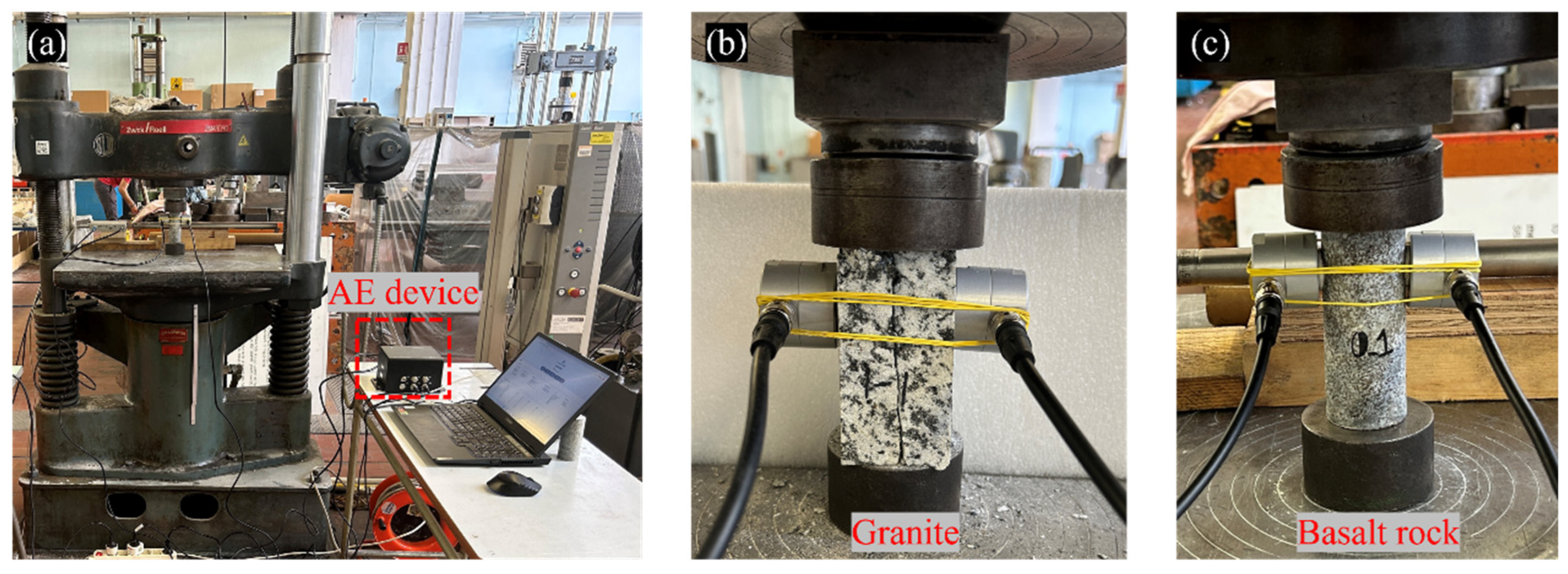
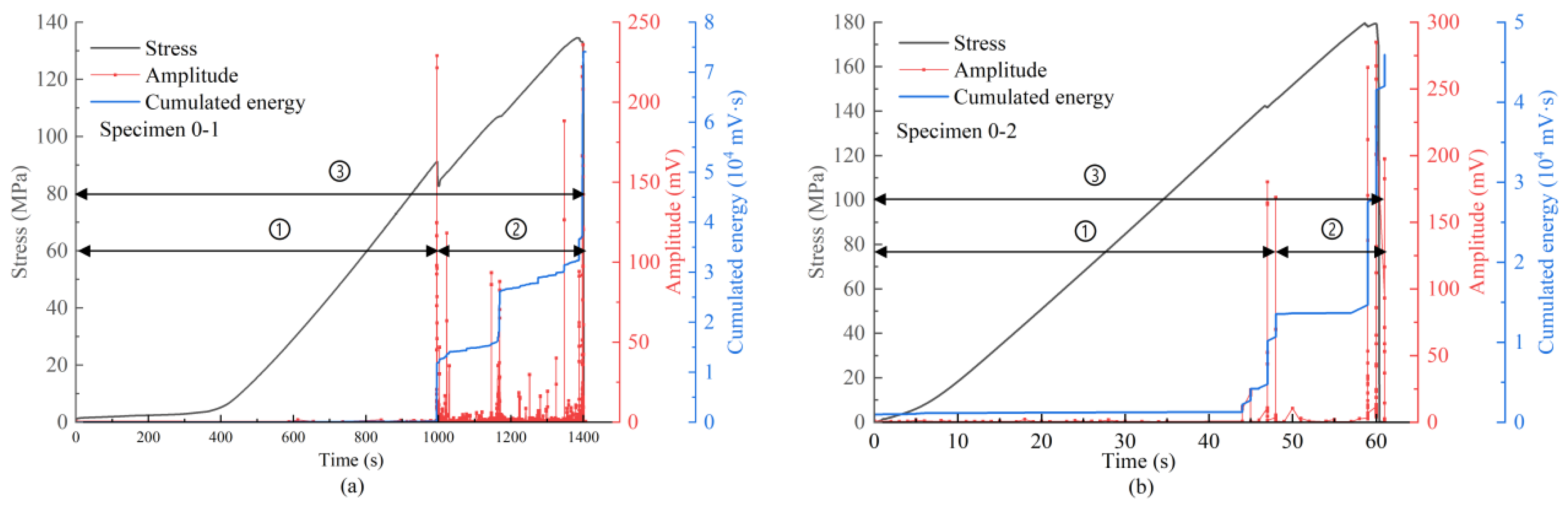
AE parameters effectively reflect the rock failure process, providing essential information about the rock’s condition and facilitating the study and understanding of rock failure processes. The stress and AE parameter evolution curves during uniaxial compression of basalt and granite rocks can be observed in Figure 3.

Clearly, basalt rocks exhibit higher uniaxial compressive strength due to having fewer pores in the samples. In contrast, granite rocks, characterized by a relatively higher number of pores, exhibit lower uniaxial compressive strength and produce many AE signals.

We can observe that each stress drop is accompanied by high-amplitude AE signals. Before the initial stress drop, the sample absorbs energy continuously without undergoing failure, resulting in fewer AE signals. During the stress drop, the sample releases some of its energy, including dissipative and emitted energy, leading to higher AE amplitudes and energy. After the stress drop, internal cracks within the sample begin to merge and propagate, eventually releasing all the stored energy, causing catastrophic collapse. This stage generates numerous and densely packed AE signals, with the highest AE energy at the time of collapse. Therefore, AE parameters are closely linked to crack development and can simultaneously characterize energy variations in the rock instability process.

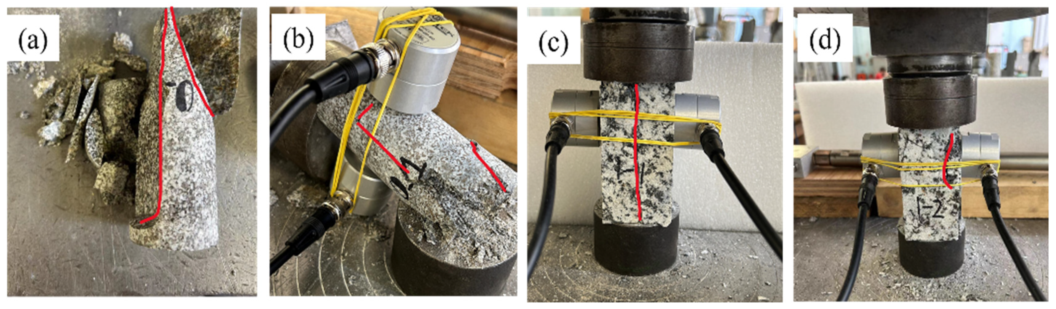
Figure 4 presents images after experiments on two types of rocks, with the red line indicating the main fracture direction of the specimen. It is worth noting that, as evident from Figure 4, fracture occurred after the specimen reached strength, with the primary mode of failure being cleavage. During the testing process, significant cleavage fractures occurred along the direction of the red line, revealing the brittle characteristics of the rock.

3.2. b-Value and γ-Value

3.2.1. Calculation of AE b-Value

The seismic b-value was initially introduced by Gutenberg-Richter [14] and later was progressively utilized to study the evolution of damage and fracture processes in solid materials using the AE b-value. The calculation of the b-value is based on Equation (2):

$${log}_{10}N\left(N\ge M\right)=a-bM,$$

(2)

where M is the magnitude of AE signals, and a is constant. N is the number of earthquakes with a magnitude greater than or equal to M.

The relationship between AE amplitude and magnitude, considering that the maximum signal peak amplitude can be expressed in dB as $A_{dB}=20{log}_{10}\left(\frac{V_{max}}{V_{ref}}\right)$, can be calculated using Equation (3):

$$M={log}_{10}\left(\frac{V_{max}}{V_{ref}}\right),$$

(3)

where V_ref is a reference amplitude (in this study, taken as 1 μV).

Therefore, the AE b-value can be represented by Equation (4):

$${log}_{10}N\left(N\ge M\right)=a-b·{\mathit{log}}_{10}\left(\frac{V_{max}}{V_{ref}}\right)$$

(4)

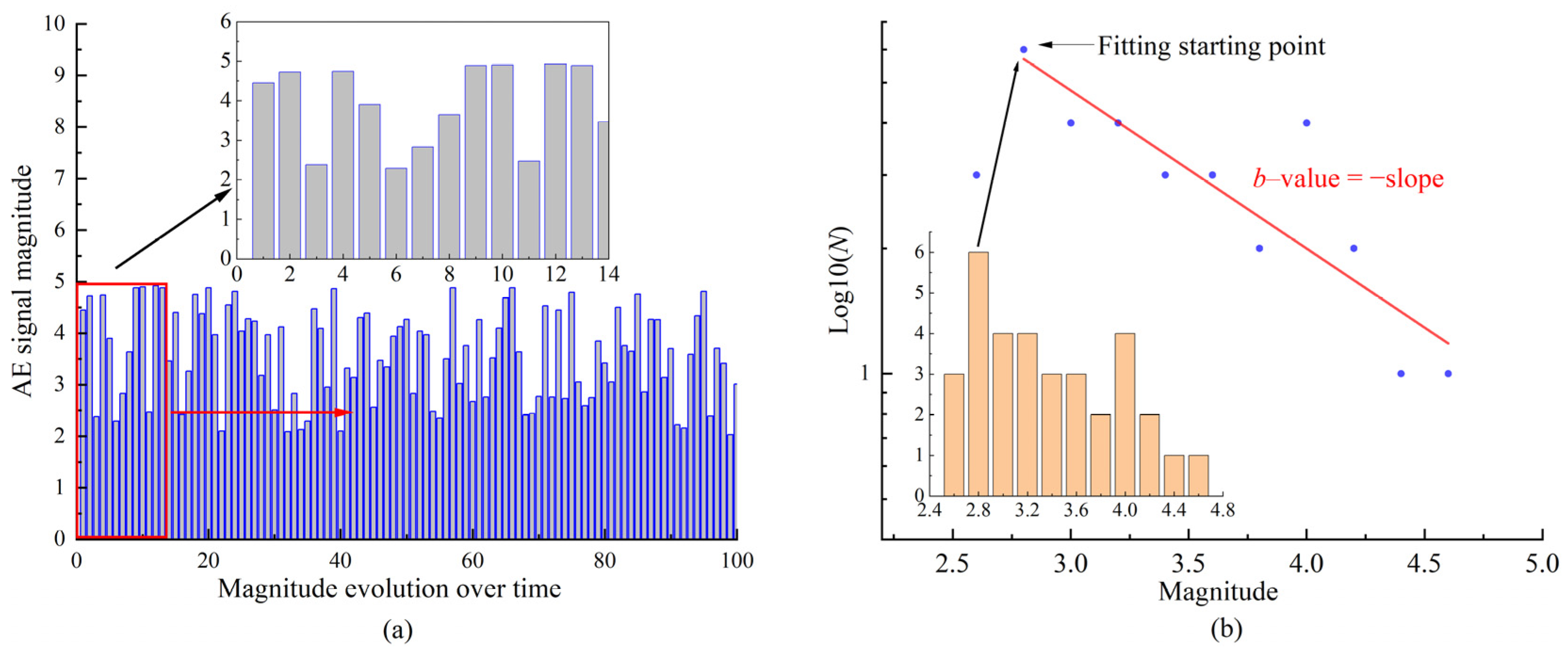
According to Equation (4), it is evident that the b-value can be calculated based on the relationship between AE amplitude and their frequency. By linearly fitting log₁₀N and M, the negative of the slope is the desired AE b-value. To clearly depict the evolution of the b-value over time, this study applied time windows to the acquired data. Subsequently, the b-value for each specific time window was calculated. The detailed calculation steps are illustrated in Figure 5.

3.2.2. Calculation of AE γ-Value

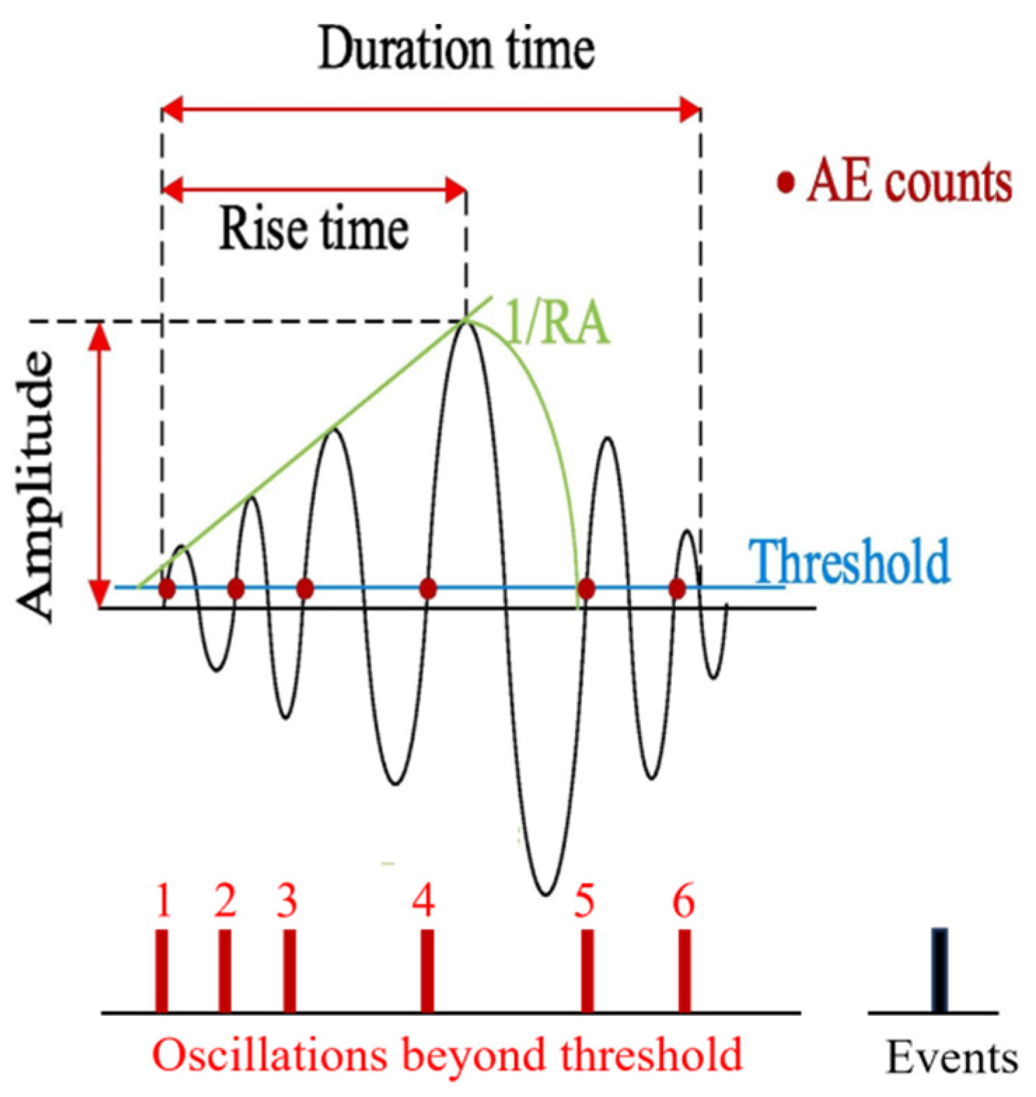
A potential precursor indicator for studying the compressive failure process of rocks is known as the FNS method. It follows a power-law form of 1/f^γ, where f represents frequency, and γ is a characteristic parameter of frequency. This γ-value can capture variations in complex systems within time series data. When γ = 1, the AE signal follows the pattern of 1/f noise, which is also known as “pink noise”. When rocks produce a significant number of AE, it indicates an unstable state and the AE signal consistently exhibits the 1/f characteristic in the power spectrum. When rocks generate fewer AE, it implies better rock integrity, and the sample is in a stable state, with γ approaching 0.

The calculation method for the characteristic parameter γ-value is as follows: Assuming the waveform of AE at any time t is represented by f(t), then the Fourier transform of AE is described as Equation (5):

$$F\left(f\right)={\int }_{-\infty }^{\infty }f\left(t\right)e^{-jft}dt,$$

(5)

where f is frequency. The power spectral density (PSD) is given by Equation (6):

$$PSD\left(f\right)={\left|F\left(f\right)\right|}^2,$$

(6)

Taking the natural logarithm of both sides of Equation (6):

$${\mathit{log}}_{10}\left(PSD\right)=c+\gamma ·{\mathit{log}}_{10}\left(f\right).$$

(7)

In Equation (7), the γ-value is the parameter we are seeking.

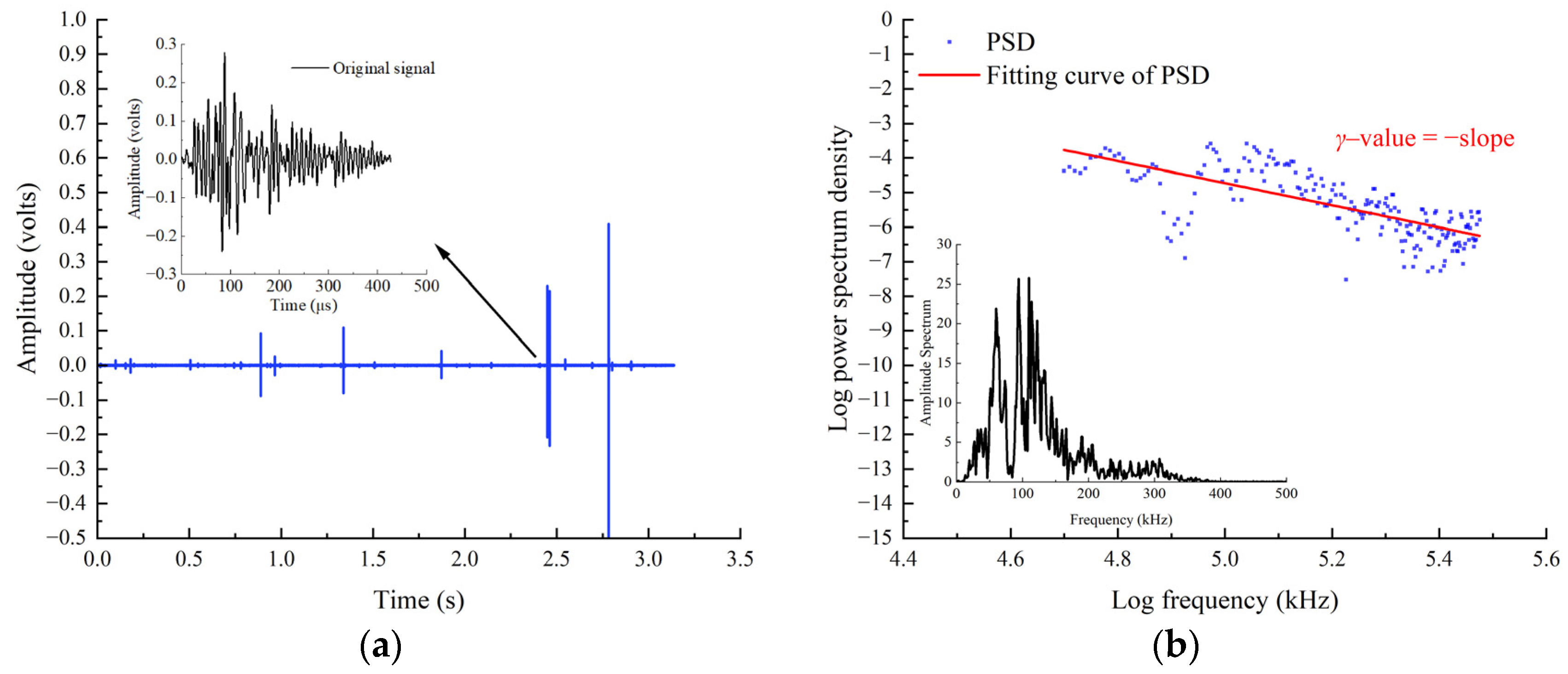
According to Equation (7), the γ-value can be calculated using the power spectrum of AE. By linearly fitting log₁₀(PSD) and log₁₀(f), the negative slope of the line is the γ-value. To demonstrate the trend of γ-value over time, time windows were applied to the experimental AE waveform data. The power spectrum was calculated for each time window, and γ-value were determined sequentially. The calculation process is illustrated in Figure 6.

3.3. b-Value and γ-Value Analysis

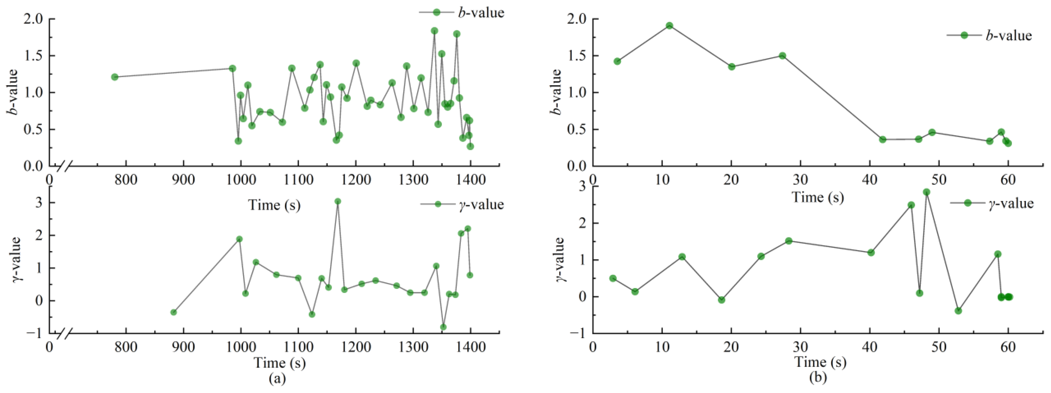
Based on the calculation methods outlined in Section 3.2, the evolution curves of the b-value and γ-value during the entire loading process are depicted in Figure 7. Since both basalt and granite rocks exhibited similar results, this paper only displays the results for basalt rock Samples 0–1 and 0–2. Combining the analysis of stress and AE curves (as shown in Figure 3), we can observe that for Specimen 0–1, stress drops occurred at 996 s and 1172 s. At these moments, high-amplitude AE signals were generated, resulting in a sudden decrease in the b-value (0.3), while the γ-value concurrently increased rapidly. At 1399 s, Specimen 0–1 collapsed, leading to a decrease in the b-value and a sharp increase in the γ-value. Notably, whenever stress drops and sudden collapses occurred in the specimens, the b-value and γ-value consistently exhibited opposing trends. Similar patterns were observed in Specimen 0–2. This indicates that both the b-value and γ-value can effectively reflect the rock damage process, especially showing sensitivity to stress drops. When specimens undergo catastrophic collapse, both parameters undergo significant changes, thus serving as valuable precursor indicators of rock catastrophic instability.

Compared to Specimen 0–1, the b-value of Specimen 0–2 exhibits an overall trend of fluctuating decline, whereas the b-value of Specimen 0–1 experiences multiple sudden drops. Simultaneously, the γ-value of Specimen 0–2 shows a continuous overall increase, while Specimen 0–1 only undergoes sudden increases at certain moments. This discrepancy arises from the differences between the two samples. The scale of crack propagation during the rock failure process is significantly related to the AE signals. The generation of microcracks corresponds to signals with low amplitude and high frequency, while the occurrence of penetrating cracks, macrocracks, and collapse-induced unstable cracks corresponds to signals with high amplitude and low frequency in AE.

According to Equation (2), the b-value of AE is entirely dependent on the relationship between AE magnitude and frequency. Signals with high amplitude and low frequency correspond to lower b-value, whereas signals with low amplitude and high frequency correspond to higher b-value. Therefore, the b-value can reflect the scale of rock crack propagation from a time-domain perspective. Similarly, according to Equation (3), the magnitude of the γ-value in AE is related to frequency and power spectral density. Signals with low amplitude and high frequency correspond to high power spectral density and high amplitude. Thus, the γ-value can reflect the scale of rock crack propagation from a frequency-domain perspective.

After the initial stress drop, internal cracks develop in Specimen 0–1, continuously generating signals with high amplitude as stress increases. In contrast, Specimen 0–2 does not further expand cracks after the initial stress drop, producing signals with high amplitude only when complete failure occurs. This discrepancy contributes to the differences between the parameters of the two specimens.

3.4. β_t-Value

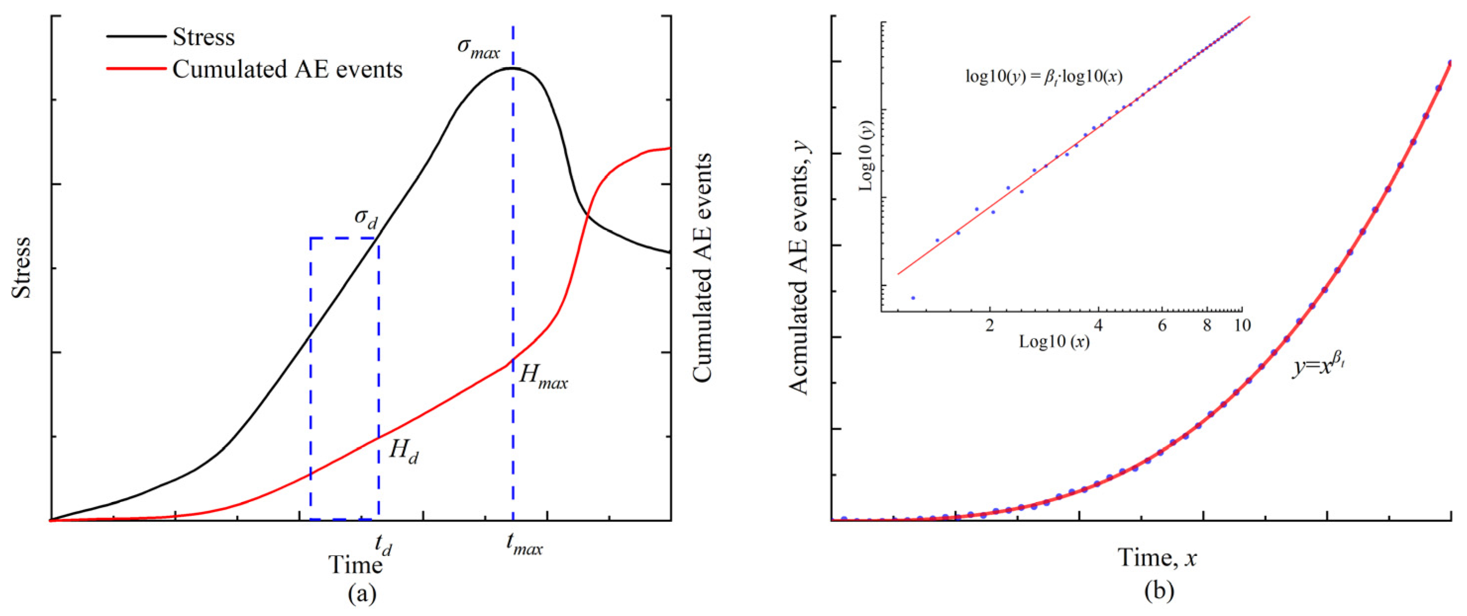
3.4.1. Calculation of β_t-Value

The energy release W measured by the AE technique follows the time-effect law [27]:

$$W\left(t\right)\propto H\left(t\right)\propto t^{{\beta }_t},$$

(8)

In which t represents the test time, H is the cumulative number of detected AE events, and β_t represents the exponent of the release energy scale. The extent of material damage and failure can be expressed as a function of the number of AE events and time:

$$\eta =\frac{H}{H_{\mathit{max}}}={\left(\frac{t}{t_{\mathit{max}}}\right)}^{{\beta }_t},$$

(9)

Taking the natural logarithm of both sides of Equation (9):

$$\mathit{log}\left(\frac{H}{H_{\mathit{max}}}\right)={\beta }_t\mathit{log}\left(\frac{t}{t_{\mathit{max}}}\right).$$

(10)

where H_max represents the total number of AE events during the monitoring period when the stress reaches its peak value σ_max, and t_max represents the corresponding monitoring duration. To analyze the distribution patterns of β_t at different stress stages, we calculate β_t separately for different stages of AE. For a specific time interval, β_t can be determined using Equation (11).

$$\mathit{log}\left(\frac{H}{H_d}\right)={\beta }_t\mathit{log}\left(\frac{t}{t_d}\right).$$

(11)

where H_d and t_d represent the cumulative AE counts and monitoring duration within the selected time interval. A schematic diagram illustrating the calculation of β_t is shown in Figure 8.

3.4.2. β_t-Value Analysis

Previous research has revealed that when β_t is less than 1, the specimen is in a stable state; when β_t equals 1, it is in a metastable state; and when β_t is greater than 1, it is in an unstable state [27]. To process the acquired AE signals using the calculation method described in Section 3.4.1, we calculate the β_t-value for different stress stages. Based on the stress distribution characteristics, the data are segmented for analysis.

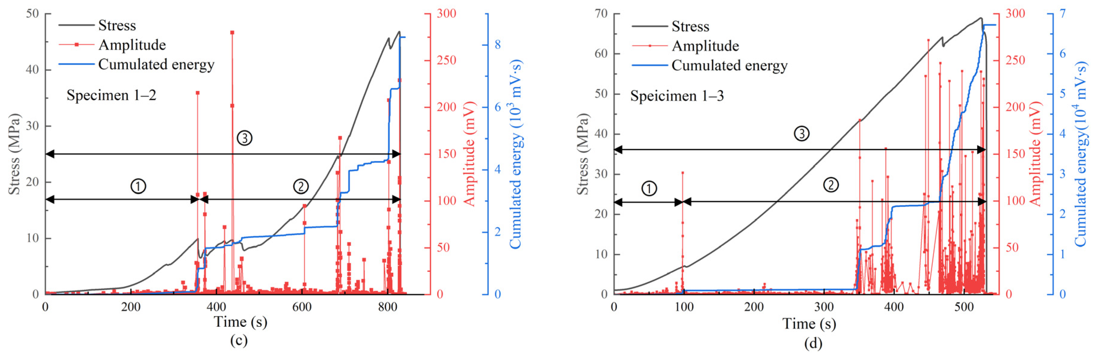
Before the initial stress drop, due to compaction or linear elastic behavior, the specimen generates fewer cracks, resulting in fewer AE signals. After the stress drop, the specimen’s damage increases, leading to more AE signals. Therefore, we use the initial stress drop as the dividing point, dividing the entire loading stage into three phases: Stage ① extends from the beginning to the first stress drop, Stage ② spans from the first stress drop to the final failure, and Stage ③ encompasses the entire loading stage, as illustrated in Figure 3.

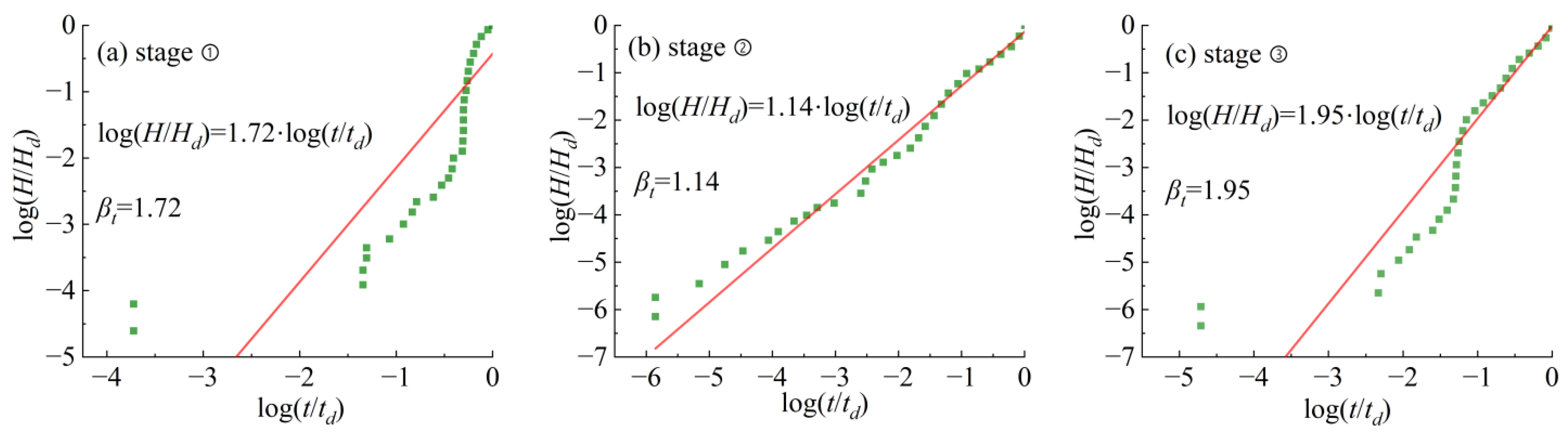
This paper uses a 0–1 specimen as an example to illustrate the changes in β_t-value at different AE stages, as shown in Figure 9. From Figure 9a, it can be observed that in Stage ①, the β_t-value is 1.72. This phase includes a stress drop, during which the rock releases a significant amount of energy, resulting in a higher occurrence of AE signals, indicating an unstable state. In Stage ②, the β_t-value is 1.14, which is close to 1. In this phase, AE signals are relatively dense, indicating that the specimen is in a metastable state. In Stage ③, the β_t-value is 1.95, encompassing the entire loading process of the specimen, and it ultimately experiences a catastrophic failure.

β_t-value calculations were performed for all specimens, and the results are shown in

Table 3. β_t-value at different stages.

Specimen	Stage	t/s	βt
0–1	①	800–1000	1.72
	②	1000–1400	1.14
	③	800–1400	1.95
0–2	①	0–50	0.98
	②	50–61	1.76
	③	0–61	1.07
1–2	①	0–380	1.32
	②	380–840	0.97
	③	0–840	1.59
1–3	①	0–105	2.27
	②	105–500	1.16
	③	0–540	1.4

. In Stages ① and ③, the β_t-value is greater than 1, indicating that these two stages are both unstable. The experimental results for these two stages also contain significant stress drops, confirming the consistency between the calculated results and the experimental data. As for Stage ②, the β_t-value for the 0–1, 1–2, and 1–3 specimens are all near 1, while the 0–2 specimen’s β_t-value is greater than 1. This variation is related to the different AE behaviors of the specimens.

For the 0–1, 1–2, and 1–3 specimens, damage continually intensifies after the first stress drop, leading to a continuous generation of AE signals. In contrast, the 0–2 specimen only produces signals at the moment of collapse after the initial stress drop.

According to Equation (11), it is evident that the value of β_t-value is solely dependent on time and the number of AE events. It reflects the relative rate of AE signal generation concerning time. Within a specific time interval, if AE signals continue to be generated, and considering signal amplitude, time is also continuously changing, resulting in a β_t-value approximately equal to 1. However, it is clear that during the initial loading stage of any specimen, if there is a continuous generation of AE signals within a certain time period, the calculation based on Equation (11) would also yield a β_t-value close to 1. However, in this stage, it is actually a stable state.

Therefore, the criterion for determining the instability of material damage and failure based on β_t-value is as follows:

• β_t < 1: The specimen structure is in a stable state.
• β_t ≈ 1: The specimen structure can be in both stable and unstable states.
• β_t > 1: The specimen structure is in an unstable state.

3.5. The Relationship between b-Value, γ-Value, and β_t-Value

From the above analysis, it is evident that the values of b, γ, and β_t can all be used to analyze the material’s damage process and assess whether the specimen is on the verge of catastrophic collapse. This section explores the relationships among these three indicators.

The relationship between AE amplitude and PSD can be explained using Fourier transformation. Fourier transformation converts a time-domain signal into a frequency-domain signal, during which the temporal information of the signal is transformed into frequency-domain information. PSD represents the energy magnitude at different signal frequencies, with larger amplitudes typically corresponding to higher PSD. Additionally, higher AE amplitudes are associated with a higher number of AE events. Assuming the following relationship:

$$A\propto PSD\propto \frac{H}{H_m}$$

(12)

Therefore, by performing equivalent substitutions based on Equations (4), (7) and (11), we can derive the relationship between b and γ:

$${log}_{10}N\left(N\ge M\right)=a-b{k}_1\left(c+\gamma ·\mathit{log}\left(f\right)\right),$$

(13)

$$b=\frac{a-{log}_{10}N\left(N\ge M\right)}{k_1\left(c+\gamma ·\mathit{log}\left(f\right)\right)}.$$

(14)

where k₁ is the proportionality coefficient between A and PSD, and k₁ is greater than 0. Similarly, we can obtain the relationship between b and β_t:

$${log}_{10}N\left(N\ge M\right)=a-b{k}_2\left({\beta }_t{log}_{10}\left(\frac{t}{t_{\mathit{max}}}\right)\right),$$

(15)

$$b=\frac{a-{log}_{10}N\left(N\ge M\right)}{k_2\left({\beta }_t{log}_{10}\left(\frac{t}{t_{\mathit{max}}}\right)\right)}$$

(16)

where k₂ is the proportionality coefficient between A and log₁₀(H/H_max), k₂ is less than 0. From Equations (13) to (16), it is evident that the b-value is inversely proportional to both γ-value and β_t-value. This is also consistent with the experimental results presented in this paper.

3.6. Discussion

This paper analyzes the variations in the AE b-value and the characteristic parameter γ-value using the flicker noise spectrum method during the process of rock failure under uniaxial compression. Simultaneously, the study investigates the relationship between the AE events and loading time on a time scale. By comparing with existing AE b-value, the research emphasizes exploring the potential of γ and β_t values as indicators for predicting dynamic hazards in rocks. These research findings provide a fresh perspective for understanding the fracture and instability behavior of rocks, offering theoretical support for predicting dynamic hazards in these materials. In this section, an analysis is conducted on the relationships and disparities between the results of this study and existing research, along with the reasons behind these disparities.

Descherevsky [28] and Moura [29] have observed interesting 1/f (γ = 1) scaling in the power spectra of monitoring signals as they transition from a critical state to catastrophic failure. The consistency of these findings with our study demonstrates relatively consistent results across different research domains. However, it is worth noting that this paper also found some other interesting phenomena. In this paper, when the catastrophic failure of rock occurs, γ is not around 1.0 but exceeds 1.0, which seems to indicate that the failure process of rock does not always satisfy the law of 1/f noise (γ = 1).

This is related to the window length used in calculating the γ-value. Similar to the b-value, calculating the γ-value requires an appropriate window length. This is because the γ-value reflects the relationship between the power spectrum of the signal over a certain time interval and its frequency. If the time window is too small, the calculated results may not effectively represent the frequency-domain characteristics of that time period. On the other hand, if the time window is too large, it cannot accurately reflect the real-time damage process of rocks during the loading process.

The proposed β_t-value in this work can reflect the evolution of rock damage processes over time scales. Previous research [30] suggested that the specimen is in a quasi-stable state when the β_t-value is 1. Interestingly, the findings of this study indicate that when the β_t-value is 1, the specimen is in a stable or quasi-stable state. This is because the β_t-value is closely associated with the number of AE events and the loading time. Even if the specimen is in a stable state, there may be a phase where the AE amplitude is small, but the number of AE events and time increase simultaneously, resulting in a β_t-value of 1. In such cases, the specimen is considered to be in a stable state.

4. Conclusions

This paper conducted uniaxial compression tests on basalt rock and granite while also collecting AE data throughout the entire loading process. Based on AE analysis, the distribution patterns of b-value, γ-value, and β_t-value during the rock-loading process were investigated, and their relationships were explored. The main conclusions obtained are as follows:

(1)

AE b-value, γ-value, and β_t-values monitored during the uniaxial compression process of the rock can effectively reflect the evolution of rock damage. These three values can be used to assess whether the rock is approaching catastrophic failure.

(2)

There is a negative correlation between the b-value and the γ-value, as well as between the b-value and the β_t-value.

(3)

The b-value, γ-value, and β_t-value, as precursory indicators of rock instability and catastrophic collapse, provide a theoretical and experimental foundation for the prevention and control of dynamic hazards in deep mining.